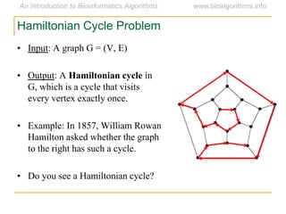
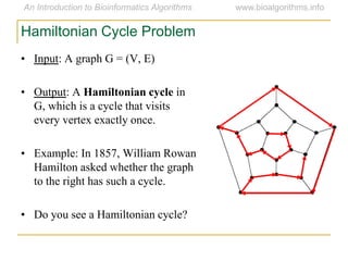
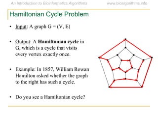
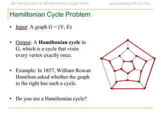
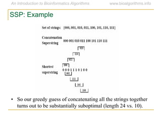
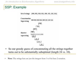
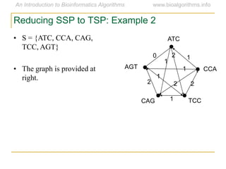
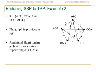
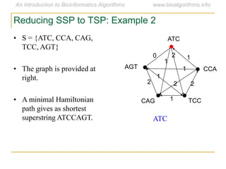
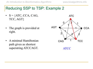
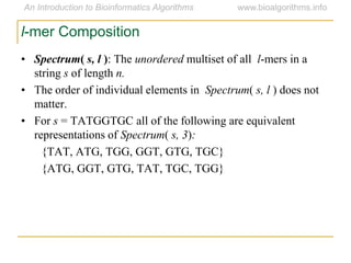
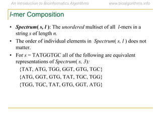
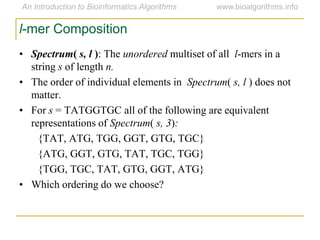
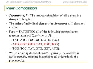
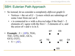
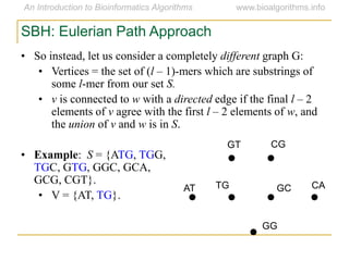
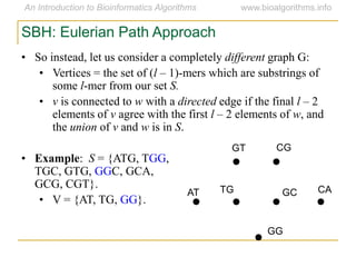
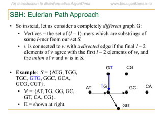
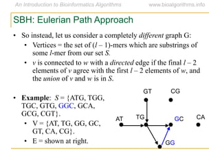
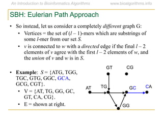
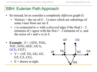
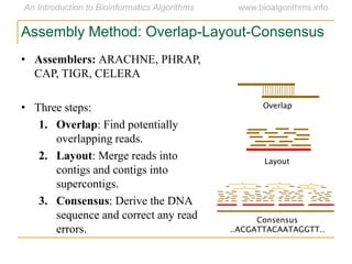
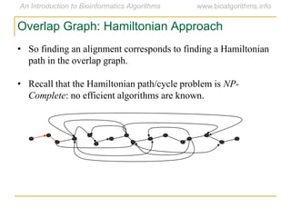
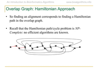
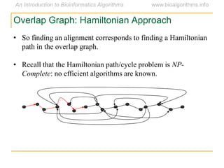
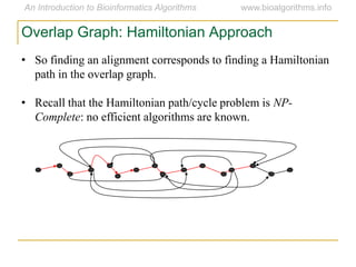
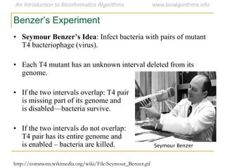
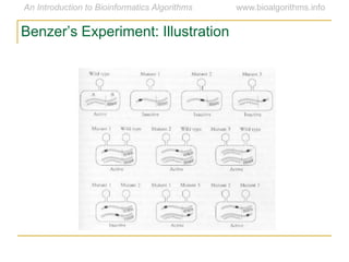
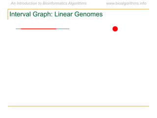
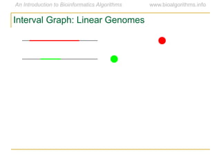
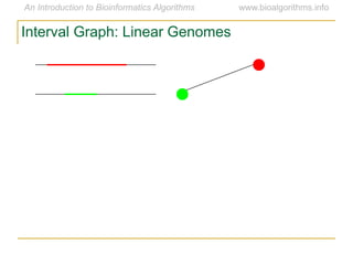
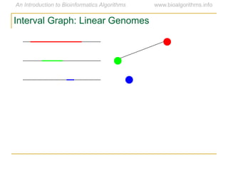
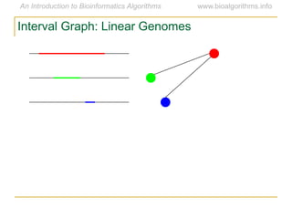
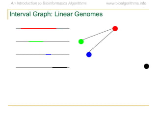
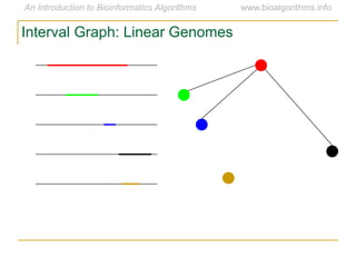
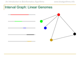
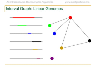
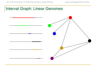
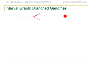
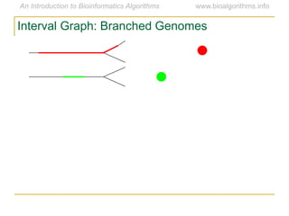
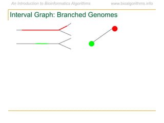
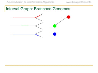
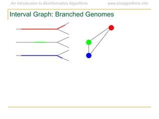
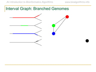
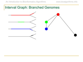
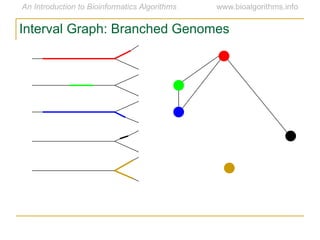
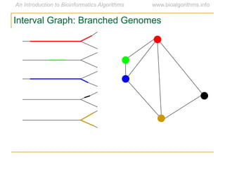
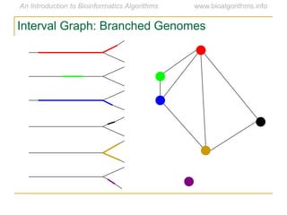
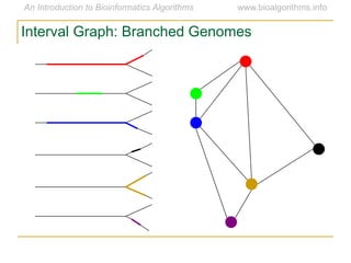
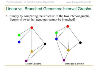
Graph algorithms have important applications in bioinformatics. Seymour Benzer used graph theory and interval graphs to study the structure of viral genomes. Through his experiment infecting bacteria with pairs of disabled bacteriophages, Benzer was able to show that the genome of these viruses was linear rather than branched based on whether the interval graph formed was interval or not. This provided insight into viral genome structure using mathematical concepts like graphs and intervals.

1. Graph Algorithms
in Bioinformatics

2. Outline
1. Introduction to Graph Theory
2. The Hamiltonian & Eulerian Cycle Problems
3. Basic Biological Applications of Graph Theory
4. DNA Sequencing
5. Shortest Superstring & Traveling Salesman Problems
6. Sequencing by Hybridization
7. Fragment Assembly & Repeats in DNA
8. Fragment Assembly Algorithms

3. Section 1:
Introduction to Graph
Theory

4. Knight Tours
• Knight Tour Problem: Given an
8 x 8 chessboard, is it possible to
find a path for a knight that visits
every square exactly once and
returns to its starting square?
• Note: In chess, a knight may move
only by jumping two spaces in one
direction, followed by a jump one
space in a perpendicular direction.
http://www.chess-poster.com/english/laws_of_chess.htm

5. 9th Century: Knight Tours Discovered

6. • 1759: Berlin Academy of Sciences
proposes a 4000 francs prize for the
solution of the more general problem
of finding a knight tour on an N x N
chessboard.
• 1766: The problem is solved by
Leonhard Euler (pronounced ―Oiler‖).
• The prize was never awarded since
Euler was Director of Mathematics
at Berlin Academy and was
deemed ineligible.
18th Century: N x N Knight Tour Problem
Leonhard Euler
http://commons.wikimedia.org/wiki/File:Leonhard_Euler_by_Handmann.png

7. • A graph is a collection (V, E) of two sets:
• V is simply a set of objects, which we
call the vertices of G.
• E is a set of pairs of vertices which
we call the edges of G.
Introduction to Graph Theory

8. • A graph is a collection (V, E) of two sets:
• V is simply a set of objects, which we
call the vertices of G.
• E is a set of pairs of vertices which
we call the edges of G.
• Simpler: Think of G as a network:
Introduction to Graph Theory
http://uh.edu/engines/epi2467.htm

9. • A graph is a collection (V, E) of two sets:
• V is simply a set of objects, which we
call the vertices of G.
• E is a set of pairs of vertices which
we call the edges of G.
• Simpler: Think of G as a network:
• Nodes = vertices
Introduction to Graph Theory
http://uh.edu/engines/epi2467.htm
Vertex

10. • A graph is a collection (V, E) of two sets:
• V is simply a set of objects, which we
call the vertices of G.
• E is a set of pairs of vertices which
we call the edges of G.
• Simpler: Think of G as a network:
• Nodes = vertices
• Edges = segments connecting the
nodes
Introduction to Graph Theory
http://uh.edu/engines/epi2467.htm
Vertex
Edge

11. Section 2:
The Hamiltonian &
Eulerian Cycle Problems

12. • Input: A graph G = (V, E)
• Output: A Hamiltonian cycle in
G, which is a cycle that visits
every vertex exactly once.
Hamiltonian Cycle Problem

13. • Input: A graph G = (V, E)
• Output: A Hamiltonian cycle in
G, which is a cycle that visits
every vertex exactly once.
• Example: In 1857, William Rowan
Hamilton asked whether the graph
to the right has such a cycle.
Hamiltonian Cycle Problem

14. • Input: A graph G = (V, E)
• Output: A Hamiltonian cycle in
G, which is a cycle that visits
every vertex exactly once.
• Example: In 1857, William Rowan
Hamilton asked whether the graph
to the right has such a cycle.
• Do you see a Hamiltonian cycle?
Hamiltonian Cycle Problem

15. • Input: A graph G = (V, E)
• Output: A Hamiltonian cycle in
G, which is a cycle that visits
every vertex exactly once.
• Example: In 1857, William Rowan
Hamilton asked whether the graph
to the right has such a cycle.
• Do you see a Hamiltonian cycle?
Hamiltonian Cycle Problem

16. • Input: A graph G = (V, E)
• Output: A Hamiltonian cycle in
G, which is a cycle that visits
every vertex exactly once.
• Example: In 1857, William Rowan
Hamilton asked whether the graph
to the right has such a cycle.
• Do you see a Hamiltonian cycle?
Hamiltonian Cycle Problem

17. • Input: A graph G = (V, E)
• Output: A Hamiltonian cycle in
G, which is a cycle that visits
every vertex exactly once.
• Example: In 1857, William Rowan
Hamilton asked whether the graph
to the right has such a cycle.
• Do you see a Hamiltonian cycle?
Hamiltonian Cycle Problem

18. • Input: A graph G = (V, E)
• Output: A Hamiltonian cycle in
G, which is a cycle that visits
every vertex exactly once.
• Example: In 1857, William Rowan
Hamilton asked whether the graph
to the right has such a cycle.
• Do you see a Hamiltonian cycle?
Hamiltonian Cycle Problem

19. • Input: A graph G = (V, E)
• Output: A Hamiltonian cycle in
G, which is a cycle that visits
every vertex exactly once.
• Example: In 1857, William Rowan
Hamilton asked whether the graph
to the right has such a cycle.
• Do you see a Hamiltonian cycle?
Hamiltonian Cycle Problem

20. • Input: A graph G = (V, E)
• Output: A Hamiltonian cycle in
G, which is a cycle that visits
every vertex exactly once.
• Example: In 1857, William Rowan
Hamilton asked whether the graph
to the right has such a cycle.
• Do you see a Hamiltonian cycle?
Hamiltonian Cycle Problem

21. • Input: A graph G = (V, E)
• Output: A Hamiltonian cycle in
G, which is a cycle that visits
every vertex exactly once.
• Example: In 1857, William Rowan
Hamilton asked whether the graph
to the right has such a cycle.
• Do you see a Hamiltonian cycle?
Hamiltonian Cycle Problem

22. • Input: A graph G = (V, E)
• Output: A Hamiltonian cycle in
G, which is a cycle that visits
every vertex exactly once.
• Example: In 1857, William Rowan
Hamilton asked whether the graph
to the right has such a cycle.
• Do you see a Hamiltonian cycle?
Hamiltonian Cycle Problem

23. • Input: A graph G = (V, E)
• Output: A Hamiltonian cycle in
G, which is a cycle that visits
every vertex exactly once.
• Example: In 1857, William Rowan
Hamilton asked whether the graph
to the right has such a cycle.
• Do you see a Hamiltonian cycle?
Hamiltonian Cycle Problem

24. • Input: A graph G = (V, E)
• Output: A Hamiltonian cycle in
G, which is a cycle that visits
every vertex exactly once.
• Example: In 1857, William Rowan
Hamilton asked whether the graph
to the right has such a cycle.
• Do you see a Hamiltonian cycle?
Hamiltonian Cycle Problem

25. • Input: A graph G = (V, E)
• Output: A Hamiltonian cycle in
G, which is a cycle that visits
every vertex exactly once.
• Example: In 1857, William Rowan
Hamilton asked whether the graph
to the right has such a cycle.
• Do you see a Hamiltonian cycle?
Hamiltonian Cycle Problem

26. • Input: A graph G = (V, E)
• Output: A Hamiltonian cycle in
G, which is a cycle that visits
every vertex exactly once.
• Example: In 1857, William Rowan
Hamilton asked whether the graph
to the right has such a cycle.
• Do you see a Hamiltonian cycle?
Hamiltonian Cycle Problem

27. • Input: A graph G = (V, E)
• Output: A Hamiltonian cycle in
G, which is a cycle that visits
every vertex exactly once.
• Example: In 1857, William Rowan
Hamilton asked whether the graph
to the right has such a cycle.
• Do you see a Hamiltonian cycle?
Hamiltonian Cycle Problem

28. • Input: A graph G = (V, E)
• Output: A Hamiltonian cycle in
G, which is a cycle that visits
every vertex exactly once.
• Example: In 1857, William Rowan
Hamilton asked whether the graph
to the right has such a cycle.
• Do you see a Hamiltonian cycle?
Hamiltonian Cycle Problem

29. • Input: A graph G = (V, E)
• Output: A Hamiltonian cycle in
G, which is a cycle that visits
every vertex exactly once.
• Example: In 1857, William Rowan
Hamilton asked whether the graph
to the right has such a cycle.
• Do you see a Hamiltonian cycle?
Hamiltonian Cycle Problem

30. • Input: A graph G = (V, E)
• Output: A Hamiltonian cycle in
G, which is a cycle that visits
every vertex exactly once.
• Example: In 1857, William Rowan
Hamilton asked whether the graph
to the right has such a cycle.
• Do you see a Hamiltonian cycle?
Hamiltonian Cycle Problem

31. • Input: A graph G = (V, E)
• Output: A Hamiltonian cycle in
G, which is a cycle that visits
every vertex exactly once.
• Example: In 1857, William Rowan
Hamilton asked whether the graph
to the right has such a cycle.
• Do you see a Hamiltonian cycle?
Hamiltonian Cycle Problem

32. • Input: A graph G = (V, E)
• Output: A Hamiltonian cycle in
G, which is a cycle that visits
every vertex exactly once.
• Example: In 1857, William Rowan
Hamilton asked whether the graph
to the right has such a cycle.
• Do you see a Hamiltonian cycle?
Hamiltonian Cycle Problem

33. • Input: A graph G = (V, E)
• Output: A Hamiltonian cycle in
G, which is a cycle that visits
every vertex exactly once.
• Example: In 1857, William Rowan
Hamilton asked whether the graph
to the right has such a cycle.
• Do you see a Hamiltonian cycle?
Hamiltonian Cycle Problem

34. • Input: A graph G = (V, E)
• Output: A Hamiltonian cycle in
G, which is a cycle that visits
every vertex exactly once.
• Example: In 1857, William Rowan
Hamilton asked whether the graph
to the right has such a cycle.
• Do you see a Hamiltonian cycle?
Hamiltonian Cycle Problem

35. • Let us form a graph G = (V, E) as
follows:
• V = the squares of a chessboard
• E = the set of edges (v, w) where v
and w are squares on the
chessboard and a knight can jump
from v to w in a single move.
• Hence, a knight tour is just a
Hamiltonian Cycle in this graph!
Knight Tours Revisited

36. • Theorem: The Hamiltonian Cycle Problem is NP-Complete.
• This result explains why knight tours were so difficult to find;
there is no known quick method to find them!
Hamiltonian Cycle Problem

37. • Recall the Traveling Salesman Problem (TSP):
• n cities
• Cost of traveling from i to j
is given by c(i, j)
• Goal: Find the tour of all the
cities of lowest total cost.
• Example at right: One
busy salesman!
• So we might like to think of the Hamiltonian Cycle Problem as a
TSP with all costs = 1, where we have some edges missing (there
doesn’t always exist a flight between all pairs of cities).
Hamiltonian Cycle Problem as TSP
http://www.ima.umn.edu/public-lecture/tsp/index.html

38. • The city of Konigsberg, Prussia (today: Kaliningrad, Russia)
was made up of both banks of a river, as well as two islands.
• The riverbanks and the islands were connected with bridges, as
follows:
• The residents wanted to know if they could take a walk from
anywhere in the city, cross each bridge exactly once, and wind
up where they started.
The Bridges of Konigsberg
http://www.math.uwaterloo.ca/navigation/ideas/Zeno/zenocando.shtml

39. • 1735: Enter Euler...his idea: compress each land area down to a
single point, and each bridge down to a segment connecting
two points.
The Bridges of Konigsberg

40. • 1735: Enter Euler...his idea: compress each land area down to a
single point, and each bridge down to a segment connecting
two points.
• This is just a graph!
The Bridges of Konigsberg
http://www.math.uwaterloo.ca/navigation/ideas/Zeno/zenocando.shtml

41. • 1735: Enter Euler...his idea: compress each land area down to a
single point, and each bridge down to a segment connecting
two points.
• This is just a graph!
• What we are looking for,
then, is a cycle in this
graph which covers each
edge exactly once.
The Bridges of Konigsberg
http://www.math.uwaterloo.ca/navigation/ideas/Zeno/zenocando.shtml

42. • 1735: Enter Euler...his idea: compress each land area down to a
single point, and each bridge down to a segment connecting
two points.
• This is just a graph!
• What we are looking for,
then, is a cycle in this
graph which covers each
edge exactly once.
• Using this setup, Euler
showed that such a cycle cannot exist.
The Bridges of Konigsberg
http://www.math.uwaterloo.ca/navigation/ideas/Zeno/zenocando.shtml

43. Eulerian Cycle Problem
• Input: A graph G = (V, E).
• Output: A cycle in G that touches every edge in E (called an
Eulerian cycle), if one exists.
• Example: At right is a
demonstration of an
Eulerian cycle.
http://mathworld.wolfram.com/EulerianCycle.html

44. Eulerian Cycle Problem
• Theorem: The Eulerian Cycle Problem can be solved in linear
time.
• So whereas finding a Hamiltonian cycle quickly becomes
intractable for an arbitrary graph, finding an Eulerian cycle is
relatively much easier.
• Keep this fact in mind, as it will become essential.

45. Section 3:
Basic Biological Applications
of Graph Theory

46. Modeling Hydrocarbons with Graphs
• Arthur Cayley studied chemical
structures of hydrocarbons in the
mid-1800s.
• He used trees (acyclic connected
graphs) to enumerate structural
isomers.
Hydrocarbon StructureArthur Cayley
http://www.scientific-web.com/en/Mathematics/Biographies/ArthurCayley01.html

47. T4 Bacteriophages: Life Finds a Way
• Normally, the T4 bacteriophage kills
bacteria
• However, if T4 is mutated (e.g., an
important gene is deleted) it gets
disabled and loses the ability to kill
bacteria
• Suppose a bacterium is infected with
two different disabled mutants–
would the bacterium still survive?
• Amazingly, a pair of disabled viruses
can still kill a bacterium.
• How is this possible? T4 Bacteriophage

48. Benzer’s Experiment
• Seymour Benzer’s Idea: Infect bacteria with pairs of mutant
T4 bacteriophage (virus).
• Each T4 mutant has an unknown interval deleted from its
genome.
• If the two intervals overlap: T4 pair
is missing part of its genome and
is disabled—bacteria survive.
• If the two intervals do not overlap:
T4 pair has its entire genome and
is enabled – bacteria are killed.
http://commons.wikimedia.org/wiki/File:Seymour_Benzer.gif
Seymour Benzer

49. Benzer’s Experiment: Illustration

50. Benzer’s Experiment and Graph Theory
• We construct an interval graph:
• Each T4 mutant forms a vertex.
• Place an edge between mutant pairs where bacteria survived
(i.e., the deleted intervals in the pair of mutants overlap)
• As the next slides show, the interval graph structure reveals
whether DNA is linear or branched.

51. Interval Graph: Linear Genomes

52. Interval Graph: Linear Genomes

53. Interval Graph: Linear Genomes

54. Interval Graph: Linear Genomes

55. Interval Graph: Linear Genomes

56. Interval Graph: Linear Genomes

57. Interval Graph: Linear Genomes

58. Interval Graph: Linear Genomes

59. Interval Graph: Linear Genomes

60. Interval Graph: Linear Genomes

61. Interval Graph: Linear Genomes

62. Interval Graph: Branched Genomes

63. Interval Graph: Branched Genomes

64. Interval Graph: Branched Genomes

65. Interval Graph: Branched Genomes

66. Interval Graph: Branched Genomes

67. Interval Graph: Branched Genomes

68. Interval Graph: Branched Genomes

69. Interval Graph: Branched Genomes

70. Interval Graph: Branched Genomes

71. Interval Graph: Branched Genomes

72. Interval Graph: Branched Genomes

73. Linear Genome Branched Genome
Linear vs. Branched Genomes: Interval Graphs
• Simply by comparing the structure of the two interval graphs,
Benzer showed that genomes cannot be branched!

74. Section 4:
DNA Sequencing

75. • Sanger Method (1977):
Labeled ddNTPs terminate
DNA copying at random
points.
• Both methods generate labeled
fragments of varying lengths
that are further electrophoresed.
• Gilbert Method (1977):
Chemical method to cleave
DNA at specific points (G,
G+A, T+C, C).
DNA Sequencing: History
Frederick Sanger Walter Gilbert

76. Sanger Method: Generating Read
1. Start at primer
(restriction site).
2. Grow DNA chain.
3. Include ddNTPs.
4. Stop reaction at all
possible points.
5. Separate products
by length, using
gel
electrophoresis.

77. Sanger Method: Sequencing
• Shear DNA into millions of
small fragments.
• Read 500 – 700 nucleotides
at a time from the small
fragments.

78. Fragment Assembly
• Computational Challenge: assemble individual short
fragments (―reads‖) into a single genomic sequence
(―superstring‖).
• Until late 1990s the so called ―shotgun fragment assembly‖ of
the human genome was viewed as an intractable problem,
because it required so much work for a large genome.
• Our computational challenge leads to the formal problem at
the beginning of the next section.

79. Section 5:
Shortest Superstring &
Traveling Salesman Problems

80. Shortest Superstring Problem (SSP)
• Problem: Given a set of strings, find a shortest string that
contains all of them.
• Input: Strings s1, s2,…., sn
• Output: A ―superstring‖ s that contains all strings
s1, s2,…., sn as substrings, such that the length of s is
minimized.

81. SSP: Example

82. SSP: Example

83. SSP: Example

84. SSP: Example
• So our greedy guess of concatenating all the strings together
turns out to be substantially suboptimal (length 24 vs. 10).

85. SSP: Example
• So our greedy guess of concatenating all the strings together
turns out to be substantially suboptimal (length 24 vs. 10).
• Note: The strings here are just the integers from 1 to 8 in base-2 notation.

86. SSP: Issues
• Complexity: NP-complete (in a few slides).
• Also, this formulation does not take into account the
possibility of sequencing errors, and it is difficult to adapt to
handle that consideration.

87. • Given strings si and sj , define overlap(si , sj ) as the length of
the longest prefix of sj that matches a suffix of si .
The Overlap Function

88. • Given strings si and sj , define overlap(si , sj ) as the length of
the longest prefix of sj that matches a suffix of si .
• Example:
• s1 = aaaggcatcaaatctaaaggcatcaaa
• s2 = aagcatcaaatctaaaggcatcaaa
The Overlap Function

89. • Given strings si and sj , define overlap(si , sj ) as the length of
the longest prefix of sj that matches a suffix of si .
• Example:
• s1 = aaaggcatcaaatctaaaggcatcaaa
• s2 = aagcatcaaatctaaaggcatcaaa
aaaggcatcaaatctaaaggcatcaaa
aaaggcatcaaatctaaaggcatcaaa
The Overlap Function

90. • Given strings si and sj , define overlap(si , sj ) as the length of
the longest prefix of sj that matches a suffix of si .
• Example:
• s1 = aaaggcatcaaatctaaaggcatcaaa
• s2 = aagcatcaaatctaaaggcatcaaa
aaaggcatcaaatctaaaggcatcaaa
aaaggcatcaaatctaaaggcatcaaa
• Therefore, overlap(s1 , s2 ) = 12.
The Overlap Function

91. Why is SSP an NP-Complete Problem?
• Construct a graph G as follows:
• The n vertices represent the n strings s1, s2,…., sn.
• For every pair of vertices si and sj , insert an edge of length
overlap( si, sj ) connecting the vertices.
• Then finding the shortest superstring will correspond to
finding the shortest Hamiltonian path in G.
• But this is the Traveling Salesman Problem (TSP), which we
know to be NP-complete.
• Hence SSP must also be NP-Complete!
• Note: We also need to show that any TSP can be formulated as a SSP (not difficult).

92. Reducing SSP to TSP: Example 1
• Take our previous set of
strings S = {000, 001, 010,
011, 100, 101, 110, 111}.

93. Reducing SSP to TSP: Example 1
• Take our previous set of
strings S = {000, 001, 010,
011, 100, 101, 110, 111}.
• Then the graph for S is
given at right.

94. Reducing SSP to TSP: Example 1
• Take our previous set of
strings S = {000, 001, 010,
011, 100, 101, 110, 111}.
• Then the graph for S is
given at right.
• One minimal Hamiltonian
path gives our previous
superstring, 0001110100.

95. Reducing SSP to TSP: Example 1
• Take our previous set of
strings S = {000, 001, 010,
011, 100, 101, 110, 111}.
• Then the graph for S is
given at right.
• One minimal Hamiltonian
path gives our previous
superstring, 0001110100.
• Check that this works!

96. Reducing SSP to TSP: Example 2
• S = {ATC, CCA, CAG,
TCC, AGT}

97. Reducing SSP to TSP: Example 2
ATC
CCA
TCC
AGT
CAG
2
2 22
1
1
1
0
1
1
• S = {ATC, CCA, CAG,
TCC, AGT}
• The graph is provided at
right.

98. Reducing SSP to TSP: Example 2
ATC
CCA
TCC
AGT
CAG
2
2 22
1
1
1
0
1
1
• S = {ATC, CCA, CAG,
TCC, AGT}
• The graph is provided at
right.
• A minimal Hamiltonian
path gives as shortest
superstring ATCCAGT.

99. Reducing SSP to TSP: Example 2
ATC
CCA
TCC
AGT
CAG
2
2 22
1
1
1
0
1
1
ATC
• S = {ATC, CCA, CAG,
TCC, AGT}
• The graph is provided at
right.
• A minimal Hamiltonian
path gives as shortest
superstring ATCCAGT.

100. Reducing SSP to TSP: Example 2
ATC
CCA
TCC
AGT
CAG
2
2 22
1
1
1
0
1
1
ATCC
• S = {ATC, CCA, CAG,
TCC, AGT}
• The graph is provided at
right.
• A minimal Hamiltonian
path gives as shortest
superstring ATCCAGT.

101. Reducing SSP to TSP: Example 2
ATC
CCA
TCC
AGT
CAG
2
2 22
1
1
1
0
1
1
ATCCA
• S = {ATC, CCA, CAG,
TCC, AGT}
• The graph is provided at
right.
• A minimal Hamiltonian
path gives as shortest
superstring ATCCAGT.

102. Reducing SSP to TSP: Example 2
ATC
CCA
TCC
AGT
CAG
2
2 22
1
1
1
0
1
1
ATCCAG
• S = {ATC, CCA, CAG,
TCC, AGT}
• The graph is provided at
right.
• A minimal Hamiltonian
path gives as shortest
superstring ATCCAGT.

103. Reducing SSP to TSP: Example 2
ATC
CCA
TCC
AGT
CAG
2
2 22
1
1
1
0
1
1
• S = {ATC, CCA, CAG,
TCC, AGT}
• The graph is provided at
right.
• A minimal Hamiltonian
path gives as shortest
superstring ATCCAGT. ATCCAGT

104. Section 6:
Sequencing By
Hybridization

105. • 1988: SBH is suggested as an an
alternative sequencing method.
Nobody believes it will ever
work.
• 1991: Light directed polymer
synthesis is developed by Steve
Fodor and colleagues.
• 1994: Affymetrix develops the
first 64-kb DNA microarray.
First microarray
prototype (1989)
First commercial
DNA microarray
prototype w/16,000
features (1994)
500,000 features
per chip (2002)
Sequencing by Hybridization (SBH): History

106. • Attach all possible DNA probes of length l to a flat surface,
each probe at a distinct known location. This set of probes is
called a DNA array.
• Apply a solution containing
fluorescently labeled DNA
fragment to the array.
• The DNA fragment hybridizes
with those probes that are
complementary to substrings
of length l of the fragment.
How SBH Works
Hybridization of a DNA Probe
http://members.cox.net/amgough/Fanconi-genetics-PGD.htm

107. How SBH Works
• Using a spectroscopic
detector, determine
which probes hybridize
to the DNA fragment to
obtain the l–mer
composition of the target
DNA fragment.
• Reconstruct the sequence
of the target DNA
fragment from the l-mer
composition.
DNA Microarray
http://www.wormbook.org/chapters/www_germlinegenomics/germlinegenomics.html

108. How SBH Works: Example
• Say our DNA fragment hybridizes to indicate that it contains
the following substrings: GCAA, CAAA, ATAG, TAGG,
ACGC, GGCA.
• Then the most logical
explanation is that our
fragment is the shortest
superstring containing
these strings!
• Here the superstring is:
ATAGGCAAACGC DNA Microarray Interpreted

109. l-mer Composition
• Spectrum( s, l ): The unordered multiset of all l-mers in a
string s of length n.
• The order of individual elements in Spectrum( s, l ) does not
matter.

110. l-mer Composition
• Spectrum( s, l ): The unordered multiset of all l-mers in a
string s of length n.
• The order of individual elements in Spectrum( s, l ) does not
matter.
• For s = TATGGTGC all of the following are equivalent
representations of Spectrum( s, 3):

111. l-mer Composition
• Spectrum( s, l ): The unordered multiset of all l-mers in a
string s of length n.
• The order of individual elements in Spectrum( s, l ) does not
matter.
• For s = TATGGTGC all of the following are equivalent
representations of Spectrum( s, 3):
{TAT, ATG, TGG, GGT, GTG, TGC}

112. l-mer Composition
• Spectrum( s, l ): The unordered multiset of all l-mers in a
string s of length n.
• The order of individual elements in Spectrum( s, l ) does not
matter.
• For s = TATGGTGC all of the following are equivalent
representations of Spectrum( s, 3):
{TAT, ATG, TGG, GGT, GTG, TGC}
{ATG, GGT, GTG, TAT, TGC, TGG}

113. l-mer Composition
• Spectrum( s, l ): The unordered multiset of all l-mers in a
string s of length n.
• The order of individual elements in Spectrum( s, l ) does not
matter.
• For s = TATGGTGC all of the following are equivalent
representations of Spectrum( s, 3):
{TAT, ATG, TGG, GGT, GTG, TGC}
{ATG, GGT, GTG, TAT, TGC, TGG}
{TGG, TGC, TAT, GTG, GGT, ATG}

114. l-mer Composition
• Spectrum( s, l ): The unordered multiset of all l-mers in a
string s of length n.
• The order of individual elements in Spectrum( s, l ) does not
matter.
• For s = TATGGTGC all of the following are equivalent
representations of Spectrum( s, 3):
{TAT, ATG, TGG, GGT, GTG, TGC}
{ATG, GGT, GTG, TAT, TGC, TGG}
{TGG, TGC, TAT, GTG, GGT, ATG}
• Which ordering do we choose?

115. l-mer Composition
• Spectrum( s, l ): The unordered multiset of all l-mers in a
string s of length n.
• The order of individual elements in Spectrum( s, l ) does not
matter.
• For s = TATGGTGC all of the following are equivalent
representations of Spectrum( s, 3):
{TAT, ATG, TGG, GGT, GTG, TGC}
{ATG, GGT, GTG, TAT, TGC, TGG}
{TGG, TGC, TAT, GTG, GGT, ATG}
• Which ordering do we choose? Typically the one that is
lexicographic, meaning in alphabetical order (think of a
phonebook).

116. • Different sequences may share a common spectrum.
• Example:
Different Sequences, Same Spectrum

Spectrum GTATCT, 2  
Spectrum GTCTAT, 2  
AT, CT, GT, TA, TC 

117. The SBH Problem
• Problem: Reconstruct a string from its l-mer composition
• Input: A set S, representing all l-mers from an (unknown)
string s.
• Output: A string s such that Spectrum( s, l ) = S
• Note: As we have seen, there may be more than one correct
answer. Determining which DNA sequence is actually correct
is another matter.

118. SBH: Hamiltonian Path Approach
• Create a graph G as follows:
• Create one vertex for each member of S.
• Connect vertex v to vertex w with a directed edge (arrow)
if the last l – 1 elements of v match the first l – 1 elements
of w.
• Then a Hamiltonian path in this graph will correspond to a
string s such that Spectrum( s, l )!

119. SBH: Hamiltonian Path Approach
• Example:
S = {ATG TGG TGC GTG GGC GCA GCG CGT}

120. SBH: Hamiltonian Path Approach
• Example:
S = {ATG TGG TGC GTG GGC GCA GCG CGT}

121. SBH: Hamiltonian Path Approach
• Example:
S = {ATG TGG TGC GTG GGC GCA GCG CGT}

122. SBH: Hamiltonian Path Approach
• Example:
S = {ATG TGG TGC GTG GGC GCA GCG CGT}

123. SBH: Hamiltonian Path Approach
• Example:
S = {ATG TGG TGC GTG GGC GCA GCG CGT}

124. SBH: Hamiltonian Path Approach
• Example:
S = {ATG TGG TGC GTG GGC GCA GCG CGT}

125. SBH: Hamiltonian Path Approach
• Example:
S = {ATG TGG TGC GTG GGC GCA GCG CGT}

126. SBH: Hamiltonian Path Approach
• Example:
S = {ATG TGG TGC GTG GGC GCA GCG CGT}

127. SBH: Hamiltonian Path Approach
• Example:
S = {ATG TGG TGC GTG GGC GCA GCG CGT}

128. SBH: Hamiltonian Path Approach
• Example:
S = {ATG TGG TGC GTG GGC GCA GCG CGT}

129. SBH: Hamiltonian Path Approach
• Example:
S = {ATG TGG TGC GTG GGC GCA GCG CGT}

130. SBH: Hamiltonian Path Approach
• Example:
S = {ATG TGG TGC GTG GGC GCA GCG CGT}

131. SBH: Hamiltonian Path Approach
• Example:
S = {ATG TGG TGC GTG GGC GCA GCG CGT}

132. SBH: Hamiltonian Path Approach
• Example:
S = {ATG TGG TGC GTG GGC GCA GCG CGT}
• There are actually two Hamiltonian paths in this graph:

133. SBH: Hamiltonian Path Approach
• Example:
S = {ATG TGG TGC GTG GGC GCA GCG CGT}
• There are actually two Hamiltonian paths in this graph:
• Path 1:

134. SBH: Hamiltonian Path Approach
• Example:
S = {ATG TGG TGC GTG GGC GCA GCG CGT}
• There are actually two Hamiltonian paths in this graph:
• Path 1: Gives the string
S =

135. SBH: Hamiltonian Path Approach
• Example:
S = {ATG TGG TGC GTG GGC GCA GCG CGT}
• There are actually two Hamiltonian paths in this graph:
• Path 1: Gives the string
S = ATG

136. SBH: Hamiltonian Path Approach
• Example:
S = {ATG TGG TGC GTG GGC GCA GCG CGT}
• There are actually two Hamiltonian paths in this graph:
• Path 1: Gives the string
S = ATGC

137. SBH: Hamiltonian Path Approach
• Example:
S = {ATG TGG TGC GTG GGC GCA GCG CGT}
• There are actually two Hamiltonian paths in this graph:
• Path 1: Gives the string
S = ATGCG

138. SBH: Hamiltonian Path Approach
• Example:
S = {ATG TGG TGC GTG GGC GCA GCG CGT}
• There are actually two Hamiltonian paths in this graph:
• Path 1: Gives the string
S = ATGCGT

139. SBH: Hamiltonian Path Approach
• Example:
S = {ATG TGG TGC GTG GGC GCA GCG CGT}
• There are actually two Hamiltonian paths in this graph:
• Path 1: Gives the string
S = ATGCGTG

140. SBH: Hamiltonian Path Approach
• Example:
S = {ATG TGG TGC GTG GGC GCA GCG CGT}
• There are actually two Hamiltonian paths in this graph:
• Path 1: Gives the string
S = ATGCGTGG

141. SBH: Hamiltonian Path Approach
• Example:
S = {ATG TGG TGC GTG GGC GCA GCG CGT}
• There are actually two Hamiltonian paths in this graph:
• Path 1: Gives the string
S = ATGCGTGGC

142. SBH: Hamiltonian Path Approach
• Example:
S = {ATG TGG TGC GTG GGC GCA GCG CGT}
• There are actually two Hamiltonian paths in this graph:
• Path 1: Gives the string
S = ATGCGTGGCA

143. SBH: Hamiltonian Path Approach
• Example:
S = {ATG TGG TGC GTG GGC GCA GCG CGT}
• There are actually two Hamiltonian paths in this graph:
• Path 1: Gives the string
S = ATGCGTGGCA
• Path 2:

144. SBH: Hamiltonian Path Approach
• Example:
S = {ATG TGG TGC GTG GGC GCA GCG CGT}
• There are actually two Hamiltonian paths in this graph:
• Path 1: Gives the string
S = ATGCGTGGCA
• Path 2: Gives the string
S =

145. SBH: Hamiltonian Path Approach
• Example:
S = {ATG TGG TGC GTG GGC GCA GCG CGT}
• There are actually two Hamiltonian paths in this graph:
• Path 1: Gives the string
S = ATGCGTGGCA
• Path 2: Gives the string
S = ATG

146. SBH: Hamiltonian Path Approach
• Example:
S = {ATG TGG TGC GTG GGC GCA GCG CGT}
• There are actually two Hamiltonian paths in this graph:
• Path 1: Gives the string
S = ATGCGTGGCA
• Path 2: Gives the string
S = ATGG

147. SBH: Hamiltonian Path Approach
• Example:
S = {ATG TGG TGC GTG GGC GCA GCG CGT}
• There are actually two Hamiltonian paths in this graph:
• Path 1: Gives the string
S = ATGCGTGGCA
• Path 2: Gives the string
S = ATGGC

148. SBH: Hamiltonian Path Approach
• Example:
S = {ATG TGG TGC GTG GGC GCA GCG CGT}
• There are actually two Hamiltonian paths in this graph:
• Path 1: Gives the string
S = ATGCGTGGCA
• Path 2: Gives the string
S = ATGGCG

149. SBH: Hamiltonian Path Approach
• Example:
S = {ATG TGG TGC GTG GGC GCA GCG CGT}
• There are actually two Hamiltonian paths in this graph:
• Path 1: Gives the string
S = ATGCGTGGCA
• Path 2: Gives the string
S = ATGGCGT

150. SBH: Hamiltonian Path Approach
• Example:
S = {ATG TGG TGC GTG GGC GCA GCG CGT}
• There are actually two Hamiltonian paths in this graph:
• Path 1: Gives the string
S = ATGCGTGGCA
• Path 2: Gives the string
S = ATGGCGTG

151. SBH: Hamiltonian Path Approach
• Example:
S = {ATG TGG TGC GTG GGC GCA GCG CGT}
• There are actually two Hamiltonian paths in this graph:
• Path 1: Gives the string
S = ATGCGTGGCA
• Path 2: Gives the string
S = ATGGCGTGC

152. SBH: Hamiltonian Path Approach
• Example:
S = {ATG TGG TGC GTG GGC GCA GCG CGT}
• There are actually two Hamiltonian paths in this graph:
• Path 1: Gives the string
S = ATGCGTGGCA
• Path 2: Gives the string
S = ATGGCGTGCA

153. SBH: A Lost Cause?
• At this point, we should be concerned about using a
Hamiltonian path to solve SBH.
• After all, recall that SSP was an NP-Complete problem, and
we have seen that an instance of SBH is an instance of SSP.
• However, note that SBH is actually a specific case of SSP, so
there is still hope for an efficient algorithm for SBH:
• We are considering a spectrum of only l-mers, and not
strings of any other length.
• Also, we only are connecting two l-mers with an edge if and
only if the overlap between them is l – 1, whereas before we
connected l-mers if there was any overlap at all.
• Note: SBH is not NP-Complete since SBH reduces to SSP, but not vice-versa.

154. SBH: Eulerian Path Approach
• So instead, let us consider a completely different graph G:
• Vertices = the set of (l – 1)-mers which are substrings of
some l-mer from our set S.
• v is connected to w with a directed edge if the final l – 2
elements of v agree with the first l – 2 elements of w, and
the union of v and w is in S.
• Example: S = {ATG, TGG,
TGC, GTG, GGC, GCA,
GCG, CGT}.

155. SBH: Eulerian Path Approach
• So instead, let us consider a completely different graph G:
• Vertices = the set of (l – 1)-mers which are substrings of
some l-mer from our set S.
• v is connected to w with a directed edge if the final l – 2
elements of v agree with the first l – 2 elements of w, and
the union of v and w is in S.
• Example: S = {ATG, TGG,
TGC, GTG, GGC, GCA,
GCG, CGT}.
• V = {AT}.
AT
GT CG
CAGCTG
GG

156. SBH: Eulerian Path Approach
• So instead, let us consider a completely different graph G:
• Vertices = the set of (l – 1)-mers which are substrings of
some l-mer from our set S.
• v is connected to w with a directed edge if the final l – 2
elements of v agree with the first l – 2 elements of w, and
the union of v and w is in S.
• Example: S = {ATG, TGG,
TGC, GTG, GGC, GCA,
GCG, CGT}.
• V = {AT, TG}.
AT
GT CG
CAGCTG
GG

157. SBH: Eulerian Path Approach
• So instead, let us consider a completely different graph G:
• Vertices = the set of (l – 1)-mers which are substrings of
some l-mer from our set S.
• v is connected to w with a directed edge if the final l – 2
elements of v agree with the first l – 2 elements of w, and
the union of v and w is in S.
• Example: S = {ATG, TGG,
TGC, GTG, GGC, GCA,
GCG, CGT}.
• V = {AT, TG, GG}.
AT
GT CG
CAGCTG
GG

158. SBH: Eulerian Path Approach
• So instead, let us consider a completely different graph G:
• Vertices = the set of (l – 1)-mers which are substrings of
some l-mer from our set S.
• v is connected to w with a directed edge if the final l – 2
elements of v agree with the first l – 2 elements of w, and
the union of v and w is in S.
• Example: S = {ATG, TGG,
TGC, GTG, GGC, GCA,
GCG, CGT}.
• V = {AT, TG, GG, GC}.
AT
GT CG
CAGCTG
GG

159. SBH: Eulerian Path Approach
• So instead, let us consider a completely different graph G:
• Vertices = the set of (l – 1)-mers which are substrings of
some l-mer from our set S.
• v is connected to w with a directed edge if the final l – 2
elements of v agree with the first l – 2 elements of w, and
the union of v and w is in S.
• Example: S = {ATG, TGG,
TGC, GTG, GGC, GCA,
GCG, CGT}.
• V = {AT, TG, GG, GC,
GT}.
AT
GT CG
CAGCTG
GG

160. SBH: Eulerian Path Approach
• So instead, let us consider a completely different graph G:
• Vertices = the set of (l – 1)-mers which are substrings of
some l-mer from our set S.
• v is connected to w with a directed edge if the final l – 2
elements of v agree with the first l – 2 elements of w, and
the union of v and w is in S.
• Example: S = {ATG, TGG,
TGC, GTG, GGC, GCA,
GCG, CGT}.
• V = {AT, TG, GG, GC,
GT, CA}.
AT
GT CG
CAGCTG
GG

161. SBH: Eulerian Path Approach
• So instead, let us consider a completely different graph G:
• Vertices = the set of (l – 1)-mers which are substrings of
some l-mer from our set S.
• v is connected to w with a directed edge if the final l – 2
elements of v agree with the first l – 2 elements of w, and
the union of v and w is in S.
• Example: S = {ATG, TGG,
TGC, GTG, GGC, GCA,
GCG, CGT}.
• V = {AT, TG, GG, GC,
GT, CA, CG}.
AT
GT CG
CAGCTG
GG

162. SBH: Eulerian Path Approach
• So instead, let us consider a completely different graph G:
• Vertices = the set of (l – 1)-mers which are substrings of
some l-mer from our set S.
• v is connected to w with a directed edge if the final l – 2
elements of v agree with the first l – 2 elements of w, and
the union of v and w is in S.
• Example: S = {ATG, TGG,
TGC, GTG, GGC, GCA,
GCG, CGT}.
• V = {AT, TG, GG, GC,
GT, CA, CG}.
• E = shown at right.
AT
GT CG
CAGCTG
GG

163. SBH: Eulerian Path Approach
• So instead, let us consider a completely different graph G:
• Vertices = the set of (l – 1)-mers which are substrings of
some l-mer from our set S.
• v is connected to w with a directed edge if the final l – 2
elements of v agree with the first l – 2 elements of w, and
the union of v and w is in S.
• Example: S = {ATG, TGG,
TGC, GTG, GGC, GCA,
GCG, CGT}.
• V = {AT, TG, GG, GC,
GT, CA, CG}.
• E = shown at right.
AT
GT CG
CAGCTG
GG

164. SBH: Eulerian Path Approach
• So instead, let us consider a completely different graph G:
• Vertices = the set of (l – 1)-mers which are substrings of
some l-mer from our set S.
• v is connected to w with a directed edge if the final l – 2
elements of v agree with the first l – 2 elements of w, and
the union of v and w is in S.
• Example: S = {ATG, TGG,
TGC, GTG, GGC, GCA,
GCG, CGT}.
• V = {AT, TG, GG, GC,
GT, CA, CG}.
• E = shown at right.
AT
GT CG
CAGCTG
GG

165. SBH: Eulerian Path Approach
• So instead, let us consider a completely different graph G:
• Vertices = the set of (l – 1)-mers which are substrings of
some l-mer from our set S.
• v is connected to w with a directed edge if the final l – 2
elements of v agree with the first l – 2 elements of w, and
the union of v and w is in S.
• Example: S = {ATG, TGG,
TGC, GTG, GGC, GCA,
GCG, CGT}.
• V = {AT, TG, GG, GC,
GT, CA, CG}.
• E = shown at right.
AT
GT CG
CAGCTG
GG

166. SBH: Eulerian Path Approach
• So instead, let us consider a completely different graph G:
• Vertices = the set of (l – 1)-mers which are substrings of
some l-mer from our set S.
• v is connected to w with a directed edge if the final l – 2
elements of v agree with the first l – 2 elements of w, and
the union of v and w is in S.
• Example: S = {ATG, TGG,
TGC, GTG, GGC, GCA,
GCG, CGT}.
• V = {AT, TG, GG, GC,
GT, CA, CG}.
• E = shown at right.
AT
GT CG
CAGCTG
GG

167. SBH: Eulerian Path Approach
• So instead, let us consider a completely different graph G:
• Vertices = the set of (l – 1)-mers which are substrings of
some l-mer from our set S.
• v is connected to w with a directed edge if the final l – 2
elements of v agree with the first l – 2 elements of w, and
the union of v and w is in S.
• Example: S = {ATG, TGG,
TGC, GTG, GGC, GCA,
GCG, CGT}.
• V = {AT, TG, GG, GC,
GT, CA, CG}.
• E = shown at right.
AT
GT CG
CAGCTG
GG

168. SBH: Eulerian Path Approach
• So instead, let us consider a completely different graph G:
• Vertices = the set of (l – 1)-mers which are substrings of
some l-mer from our set S.
• v is connected to w with a directed edge if the final l – 2
elements of v agree with the first l – 2 elements of w, and
the union of v and w is in S.
• Example: S = {ATG, TGG,
TGC, GTG, GGC, GCA,
GCG, CGT}.
• V = {AT, TG, GG, GC,
GT, CA, CG}.
• E = shown at right.
AT
GT CG
CAGCTG
GG

169. SBH: Eulerian Path Approach
• So instead, let us consider a completely different graph G:
• Vertices = the set of (l – 1)-mers which are substrings of
some l-mer from our set S.
• v is connected to w with a directed edge if the final l – 2
elements of v agree with the first l – 2 elements of w, and
the union of v and w is in S.
• Example: S = {ATG, TGG,
TGC, GTG, GGC, GCA,
GCG, CGT}.
• V = {AT, TG, GG, GC,
GT, CA, CG}.
• E = shown at right.
AT
GT CG
CAGCTG
GG

170. SBH: Eulerian Path Approach
• So instead, let us consider a completely different graph G:
• Vertices = the set of (l – 1)-mers which are substrings of
some l-mer from our set S.
• v is connected to w with a directed edge if the final l – 2
elements of v agree with the first l – 2 elements of w, and
the union of v and w is in S.
• Example: S = {ATG, TGG,
TGC, GTG, GGC, GCA,
GCG, CGT}.
• V = {AT, TG, GG, GC,
GT, CA, CG}.
• E = shown at right.
AT
GT CG
CAGCTG
GG

171. SBH: Eulerian Path Approach
• So instead, let us consider a completely different graph G:
• Vertices = the set of (l – 1)-mers which are substrings of
some l-mer from our set S.
• v is connected to w with a directed edge if the final l – 2
elements of v agree with the first l – 2 elements of w, and
the union of v and w is in S.
• Example: S = {ATG, TGG,
TGC, GTG, GGC, GCA,
GCG, CGT}.
• V = {AT, TG, GG, GC,
GT, CA, CG}.
• E = shown at right.
AT
GT CG
CAGCTG
GG

172. SBH: Eulerian Path Approach
• Key Point: A sequence reconstruction will actually correspond
to an Eulerian path in this graph.
• Recall that an Eulerian path is ―easy‖ to find (one can always
be found in linear time)…so we have found a simple solution
to SBH!
• In our example, two solutions:
AT
GT CG
CAGCTG
GG

173. SBH: Eulerian Path Approach
• Key Point: A sequence reconstruction will actually correspond
to an Eulerian path in this graph.
• Recall that an Eulerian path is ―easy‖ to find (one can always
be found in linear time)…so we have found a simple solution
to SBH!
• In our example, two solutions:
1. ATG
AT
GT CG
CAGCTG
GG

174. SBH: Eulerian Path Approach
• Key Point: A sequence reconstruction will actually correspond
to an Eulerian path in this graph.
• Recall that an Eulerian path is ―easy‖ to find (one can always
be found in linear time)…so we have found a simple solution
to SBH!
• In our example, two solutions:
1. ATGG
AT
GT CG
CAGCTG
GG

175. SBH: Eulerian Path Approach
• Key Point: A sequence reconstruction will actually correspond
to an Eulerian path in this graph.
• Recall that an Eulerian path is ―easy‖ to find (one can always
be found in linear time)…so we have found a simple solution
to SBH!
• In our example, two solutions:
1. ATGGC
AT
GT CG
CAGCTG
GG

176. SBH: Eulerian Path Approach
• Key Point: A sequence reconstruction will actually correspond
to an Eulerian path in this graph.
• Recall that an Eulerian path is ―easy‖ to find (one can always
be found in linear time)…so we have found a simple solution
to SBH!
• In our example, two solutions:
1. ATGGCG
AT
GT CG
CAGCTG
GG

177. SBH: Eulerian Path Approach
• Key Point: A sequence reconstruction will actually correspond
to an Eulerian path in this graph.
• Recall that an Eulerian path is ―easy‖ to find (one can always
be found in linear time)…so we have found a simple solution
to SBH!
• In our example, two solutions:
1. ATGGCGT
AT
GT CG
CAGCTG
GG

178. SBH: Eulerian Path Approach
• Key Point: A sequence reconstruction will actually correspond
to an Eulerian path in this graph.
• Recall that an Eulerian path is ―easy‖ to find (one can always
be found in linear time)…so we have found a simple solution
to SBH!
• In our example, two solutions:
1. ATGGCGTG
AT
GT CG
CAGCTG
GG

179. SBH: Eulerian Path Approach
• Key Point: A sequence reconstruction will actually correspond
to an Eulerian path in this graph.
• Recall that an Eulerian path is ―easy‖ to find (one can always
be found in linear time)…so we have found a simple solution
to SBH!
• In our example, two solutions:
1. ATGGCGTGC
AT
GT CG
CAGCTG
GG

180. SBH: Eulerian Path Approach
• Key Point: A sequence reconstruction will actually correspond
to an Eulerian path in this graph.
• Recall that an Eulerian path is ―easy‖ to find (one can always
be found in linear time)…so we have found a simple solution
to SBH!
• In our example, two solutions:
1. ATGGCGTGCA
AT
GT CG
CAGCTG
GG

181. SBH: Eulerian Path Approach
• Key Point: A sequence reconstruction will actually correspond
to an Eulerian path in this graph.
• Recall that an Eulerian path is ―easy‖ to find (one can always
be found in linear time)…so we have found a simple solution
to SBH!
• In our example, two solutions:
1. ATGGCGTGCA
AT
GT CG
CAGCTG
GG

182. SBH: Eulerian Path Approach
• Key Point: A sequence reconstruction will actually correspond
to an Eulerian path in this graph.
• Recall that an Eulerian path is ―easy‖ to find (one can always
be found in linear time)…so we have found a simple solution
to SBH!
• In our example, two solutions:
1. ATGGCGTGCA
2. ATG AT
GT CG
CAGCTG
GG

183. SBH: Eulerian Path Approach
• Key Point: A sequence reconstruction will actually correspond
to an Eulerian path in this graph.
• Recall that an Eulerian path is ―easy‖ to find (one can always
be found in linear time)…so we have found a simple solution
to SBH!
• In our example, two solutions:
1. ATGGCGTGCA
2. ATGC AT
GT CG
CAGCTG
GG

184. SBH: Eulerian Path Approach
• Key Point: A sequence reconstruction will actually correspond
to an Eulerian path in this graph.
• Recall that an Eulerian path is ―easy‖ to find (one can always
be found in linear time)…so we have found a simple solution
to SBH!
• In our example, two solutions:
1. ATGGCGTGCA
2. ATGCG AT
GT CG
CAGCTG
GG

185. SBH: Eulerian Path Approach
• Key Point: A sequence reconstruction will actually correspond
to an Eulerian path in this graph.
• Recall that an Eulerian path is ―easy‖ to find (one can always
be found in linear time)…so we have found a simple solution
to SBH!
• In our example, two solutions:
1. ATGGCGTGCA
2. ATGCGT AT
GT CG
CAGCTG
GG

186. SBH: Eulerian Path Approach
• Key Point: A sequence reconstruction will actually correspond
to an Eulerian path in this graph.
• Recall that an Eulerian path is ―easy‖ to find (one can always
be found in linear time)…so we have found a simple solution
to SBH!
• In our example, two solutions:
1. ATGGCGTGCA
2. ATGCGTG AT
GT CG
CAGCTG
GG

187. SBH: Eulerian Path Approach
• Key Point: A sequence reconstruction will actually correspond
to an Eulerian path in this graph.
• Recall that an Eulerian path is ―easy‖ to find (one can always
be found in linear time)…so we have found a simple solution
to SBH!
• In our example, two solutions:
1. ATGGCGTGCA
2. ATGCGTGG AT
GT CG
CAGCTG
GG

188. SBH: Eulerian Path Approach
• Key Point: A sequence reconstruction will actually correspond
to an Eulerian path in this graph.
• Recall that an Eulerian path is ―easy‖ to find (one can always
be found in linear time)…so we have found a simple solution
to SBH!
• In our example, two solutions:
1. ATGGCGTGCA
2. ATGCGTGGC AT
GT CG
CAGCTG
GG

189. SBH: Eulerian Path Approach
• Key Point: A sequence reconstruction will actually correspond
to an Eulerian path in this graph.
• Recall that an Eulerian path is ―easy‖ to find (one can always
be found in linear time)…so we have found a simple solution
to SBH!
• In our example, two solutions:
1. ATGGCGTGCA
2. ATGCGTGGCA AT
GT CG
CAGCTG
GG

190. But…How Do We Know an Eulerian Path Exists?
• A graph is balanced if for every vertex the number of
incoming edges equals to the number of outgoing edges. We
write this for vertex v as:
in(v)=out(v)
• Theorem: A connected graph is Eulerian (i.e. contains an
Eulerian cycle) if and only if each of its vertices is balanced.
• We will prove this by demonstrating the following:
1. Every Eulerian graph is balanced.
2. Every balanced graph is Eulerian.

191. Every Eulerian Graph is Balanced
• Suppose we have an Eulerian graph G. Call C the Eulerian
cycle of G, and let v be any vertex of G.
• For every edge e entering v, we can pair e with an edge leaving
v, which is simply the edge in our cycle C that follows e.
• Therefore it directly follows that in(v)=out(v) as needed, and
since our choice of v was arbitrary, this relation must hold for
all vertices in G, so we are finished with the first part.

192. Every Balanced Graph is Eulerian
• Next, suppose that we have a balanced graph G.
• We will actually construct an Eulerian cycle in G.
• Start with an arbitrary vertex v and form a path in G without
repeated edges until we reach a ―dead end,‖ meaning a vertex
with no unused edges leaving it.
• G is balanced, so every time we enter a
vertex w that isn’t v during the course of
our path, we can find an edge leaving w.
So our dead end is v and we have a cycle.

193. Every Balanced Graph is Eulerian
• We have two simple cases for our cycle, which we call C:
1. C is an Eulerian cycle  G is Eulerian  DONE.
2. C is not an Eulerian cycle.
• So we can assume that C is not an
Eulerian cycle, which means that C
contains vertices which have
untraversed edges.
• Let w be such a vertex, and start a
new path from w. Once again, we
must obtain a cycle, say C’.

194. Every Balanced Graph is Eulerian
• Combine our cycles C and C’ into a bigger cycle C* by
swapping edges at w (see figure).
• Once again, we test C*:
1. C* is an Eulerian cycle  G is Eulerian  DONE.
2. C* is not an Eulerian cycle.
• If C* is not Eulerian, we iterate our
procedure. Because G has a finite
number of edges, we must eventually
reach a point where our current cycle
is Eulerian (Case 1 above). DONE.

195. • A vertex v is semi-balanced if either in(v) = out(v) + 1 or
in(v) = out(v) – 1 .
• Theorem: A connected graph has an Eulerian path if and only
if it contains at most two semi-balanced vertices and all other
vertices are balanced.
• If G has no semi-balanced vertices, DONE.
• If G has two semi-balanced vertices, connect them with a
new edge e, so that the graph G + e is balanced and must be
Eulerian. Remove e from the Eulerian cycle in G + e to
obtain an Eulerian path in G.
• Think: Why can G not have just one semi-balanced vertex?
Euler’s Theorem: Extension

196. • Fidelity of Hybridization: It is difficult to detect differences
between probes hybridized with perfect matches and those
with one mismatch.
• Array Size: The effect of low fidelity can be decreased with
longer l-mers, but array size increases exponentially in l.
Array size is limited with current technology.
• Practicality: SBH is still impractical. As DNA microarray
technology improves, SBH may become practical in the future.
Some Difficulties with SBH

197. • Practicality Again: Although SBH is still impractical, it
spearheaded expression analysis and SNP analysis techniques.
• Practicality Again and Again: In 2007 Solexa (now Illumina)
developed a new DNA sequencing approach that generates so
many short l-mers that they essentially mimic a universal DNA
array.
Some Difficulties with SBH

198. Section 7:
Fragment Assembly &
Repeats in DNA

199. DNA
Traditional DNA Sequencing

200. DNA
Shake
Traditional DNA Sequencing

201. DNA
Shake
DNA fragments
Traditional DNA Sequencing

202. DNA
Shake
DNA fragments
Traditional DNA Sequencing

203. DNA
Shake
DNA fragments
Vector
Circular genome
(bacterium, plasmid)
Traditional DNA Sequencing

204. +
DNA
Shake
DNA fragments
Vector
Circular genome
(bacterium, plasmid)
Traditional DNA Sequencing

205. +
DNA
Shake
DNA fragments
Vector
Circular genome
(bacterium, plasmid)
Traditional DNA Sequencing

206. + =
DNA
Shake
DNA fragments
Vector
Circular genome
(bacterium, plasmid)
Traditional DNA Sequencing

207. + =
DNA
Shake
DNA fragments
Vector
Circular genome
(bacterium, plasmid)
Traditional DNA Sequencing

208. + =
DNA
Shake
DNA fragments
Vector
Circular genome
(bacterium, plasmid)
Known
location
(restriction
site)
Traditional DNA Sequencing

209. Different Types of Vectors
Vector Size of Insert (bp)
Plasmid 2,000 - 10,000
Cosmid 40,000
BAC (Bacterial Artificial
Chromosome)
70,000 - 300,000
YAC (Yeast Artificial
Chromosome)
> 300,000
Not used much
recently

210. Electrophoresis Diagrams

211. Electrophoresis Diagrams: Hard to Read

212. Reading an Electropherogram
• Reading an Electropherogram requires four processes:
1. Filtering
2. Smoothening
3. Correction for length compressions
4. A method for calling the nucleotides – PHRED

213. Shotgun Sequencing
Genomic Segment

214. Shotgun Sequencing
Cut many times at random
(hence shotgun)
Genomic Segment

215. Shotgun Sequencing
Cut many times at random
(hence shotgun)
Genomic Segment

216. Shotgun Sequencing
Cut many times at random
(hence shotgun)
Genomic Segment

217. Shotgun Sequencing
Cut many times at random
(hence shotgun)
Genomic Segment
Get one or two reads from
each segment

218. Shotgun Sequencing
Cut many times at random
(hence shotgun)
Genomic Segment
Get one or two reads from
each segment
~500 bp ~500 bp

219. Fragment Assembly
• Cover region with ~7-fold redundancy.
• Overlap reads and extend to reconstruct the original
genomic region.
Reads

220. Read Coverage
• Length of genomic segment: L
• Number of reads: n
• Length of each read: l
• Define the coverage as: C = n l / L
• Question: How much coverage is enough?
• Lander-Waterman Model: Assuming uniform distribution of
reads, C = 10 results in 1 gap in coverage per million
nucleotides.
C

221. • Repeats: A major problem for fragment assembly.
• More than 50% of human genome are repeats:
• Over 1 million Alu repeats (about 300 bp).
• About 200,000 LINE repeats (1000 bp and longer).
Repeat Repeat Repeat
Challenges in Fragment Assembly

222. • A Triazzle ® puzzle has only
16 pieces and looks simple.
• BUT… there are many
repeats!
• The repeats make it very
difficult to solve.
• This repetition is what makes
fragment assembly is so
difficult.
DNA Assembly Analogy: Triazzle
http://www.triazzle.com/

223. Repeat Type Explanation
• Low-Complexity DNA (e.g. ATATATATACATA…)
• Microsatellite repeats (a1…ak)N where k ~ 3-6
(e.g.
CAGCAGTAGCAGCACCAG)
• Gene Families genes duplicate & then diverge
• Segmental duplications ~very long, very similar copies
Repeat Classification

224. Repeat Classification
Repeat Type Explanation
•SINE Transposon Short Interspersed Nuclear
Elements
(e.g., Alu: ~300 bp long, 106
copies)
•LINE Transposon Long Interspersed Nuclear
Elements
~500 - 5,000 bp long,
200,000 copies
•LTR retroposons Long Terminal Repeats (~700 bp)

225. Section 8:
Fragment Assembly
Algorithms

226. Assembly Method: Overlap-Layout-Consensus
• Assemblers: ARACHNE, PHRAP,
CAP, TIGR, CELERA

227. Assembly Method: Overlap-Layout-Consensus
• Assemblers: ARACHNE, PHRAP,
CAP, TIGR, CELERA
• Three steps:

228. Assembly Method: Overlap-Layout-Consensus
• Assemblers: ARACHNE, PHRAP,
CAP, TIGR, CELERA
• Three steps:
1. Overlap: Find potentially
overlapping reads.
Overlap

229. Assembly Method: Overlap-Layout-Consensus
• Assemblers: ARACHNE, PHRAP,
CAP, TIGR, CELERA
• Three steps:
1. Overlap: Find potentially
overlapping reads.
2. Layout: Merge reads into
contigs and contigs into
supercontigs.
Layout
Overlap

230. Assembly Method: Overlap-Layout-Consensus
• Assemblers: ARACHNE, PHRAP,
CAP, TIGR, CELERA
• Three steps:
1. Overlap: Find potentially
overlapping reads.
2. Layout: Merge reads into
contigs and contigs into
supercontigs.
3. Consensus: Derive the DNA
sequence and correct any read
errors.
Consensus
..ACGATTACAATAGGTT..
Layout
Overlap

231. Step 1: Overlap
• Find the best match between the suffix of one read and the
prefix of another.
• Due to sequencing errors, we need to use dynamic
programming to find the optimal overlap alignment.
• Apply a filtration method to filter out pairs of fragments that
do not share a significantly long common substring.

232. TAGATTACACAGATTAC
TAGATTACACAGATTAC
|||||||||||||||||
T GA
TAGA
| ||
TACA
TAGT
||
Step 1: Overlap
• Sort all k-mers in reads (k ~ 24).
• Find pairs of reads sharing a k-mer.
• Extend to full alignment—throw away if not >95% similar.

233. • A k-mer that appears N times initiates N2 comparisons.
• For an Alu that appears 106 times, we will have 1012
comparisons – this is too many.
• Solution: Discard all k-mers that appear more than t 
Coverage, (t ~ 10)
Step 1: Overlap

234. • We next create local multiple alignments from the overlapping
reads.
TAGATTACACAGATTACTGA
TAGATTACACAGATTACTGA
TAG TTACACAGATTATTGA
TAGATTACACAGATTACTGA
TAGATTACACAGATTACTGA
TAGATTACACAGATTACTGA
TAG TTACACAGATTATTGA
TAGATTACACAGATTACTGA
Step 2: Layout

235. Step 2: Layout
• Repeats are a major challenge.
• Do two aligned fragments really overlap, or are they from two
copies of a repeat?
• Solution: repeat masking – hide the repeats!

236. Step 2: Layout
• Repeats are a major challenge.
• Do two aligned fragments really overlap, or are they from two
copies of a repeat?
• Solution: repeat masking – hide the repeats!
• Masking results in a high rate of misassembly (~20 %).

237. Step 2: Layout
• Repeats are a major challenge.
• Do two aligned fragments really overlap, or are they from two
copies of a repeat?
• Solution: repeat masking – hide the repeats!
• Masking results in a high rate of misassembly (~20 %).
• Misassembly means a lot more work at the finishing step.

238. • Repeats shorter than read length are OK.
• Repeats with more base pair differences than the sequencing
error rate are OK.
• To make a smaller portion of the genome appear repetitive, try
to:
• Increase read length
• Decrease sequencing error rate
Step 2: Layout

239. Step 3: Consensus
• A consensus sequence is derived from a profile of the
assembled fragments.
• A sufficient number of reads are required to ensure a
statistically significant consensus.
• Reading errors are corrected.

240. • Derive multiple alignment from pairwise read alignments.
• Derive each consensus base by weighted voting.
TAGATTACACAGATTACTGA TTGATGGCGTAA CTA
TAGATTACACAGATTACTGACTTGATGGCGTAAACTA
TAG TTACACAGATTATTGACTTCATGGCGTAA CTA
TAGATTACACAGATTACTGACTTGATGGCGTAA CTA
TAGATTACACAGATTACTGACTTGATGGGGTAA CTA
TAGATTACACAGATTACTGACTTGATGGCGTAA CTA
Step 3: Consensus
Multiple Alignment
Consensus String

241. • Each vertex represents a read from the original sequence.
• Vertices are connected by an edge if they overlap.
Overlap Graph: Hamiltonian Approach

242. Repeat Repeat Repeat
• Each vertex represents a read from the original sequence.
• Vertices are connected by an edge if they overlap.
Overlap Graph: Hamiltonian Approach

243. Repeat Repeat Repeat
• Each vertex represents a read from the original sequence.
• Vertices are connected by an edge if they overlap.
Overlap Graph: Hamiltonian Approach

244. Repeat Repeat Repeat
• Each vertex represents a read from the original sequence.
• Vertices are connected by an edge if they overlap.
Overlap Graph: Hamiltonian Approach

245. Repeat Repeat Repeat
• Each vertex represents a read from the original sequence.
• Vertices are connected by an edge if they overlap.
Overlap Graph: Hamiltonian Approach

246. Repeat Repeat Repeat
• Each vertex represents a read from the original sequence.
• Vertices are connected by an edge if they overlap.
Overlap Graph: Hamiltonian Approach

247. Repeat Repeat Repeat
• Each vertex represents a read from the original sequence.
• Vertices are connected by an edge if they overlap.
Overlap Graph: Hamiltonian Approach

248. Repeat Repeat Repeat
• Each vertex represents a read from the original sequence.
• Vertices are connected by an edge if they overlap.
Overlap Graph: Hamiltonian Approach

249. Repeat Repeat Repeat
• A Hamiltonian path in this graph provides a candidate assembly.
• Each vertex represents a read from the original sequence.
• Vertices are connected by an edge if they overlap.
Overlap Graph: Hamiltonian Approach

250. • So finding an alignment corresponds to finding a Hamiltonian
path in the overlap graph.
• Recall that the Hamiltonian path/cycle problem is NP-
Complete: no efficient algorithms are known.
Overlap Graph: Hamiltonian Approach

251. • So finding an alignment corresponds to finding a Hamiltonian
path in the overlap graph.
• Recall that the Hamiltonian path/cycle problem is NP-
Complete: no efficient algorithms are known.
Overlap Graph: Hamiltonian Approach

252. • So finding an alignment corresponds to finding a Hamiltonian
path in the overlap graph.
• Recall that the Hamiltonian path/cycle problem is NP-
Complete: no efficient algorithms are known.
Overlap Graph: Hamiltonian Approach

253. • So finding an alignment corresponds to finding a Hamiltonian
path in the overlap graph.
• Recall that the Hamiltonian path/cycle problem is NP-
Complete: no efficient algorithms are known.
Overlap Graph: Hamiltonian Approach

254. • So finding an alignment corresponds to finding a Hamiltonian
path in the overlap graph.
• Recall that the Hamiltonian path/cycle problem is NP-
Complete: no efficient algorithms are known.
Overlap Graph: Hamiltonian Approach

255. • So finding an alignment corresponds to finding a Hamiltonian
path in the overlap graph.
• Recall that the Hamiltonian path/cycle problem is NP-
Complete: no efficient algorithms are known.
Overlap Graph: Hamiltonian Approach

256. • So finding an alignment corresponds to finding a Hamiltonian
path in the overlap graph.
• Recall that the Hamiltonian path/cycle problem is NP-
Complete: no efficient algorithms are known.
Overlap Graph: Hamiltonian Approach

257. • So finding an alignment corresponds to finding a Hamiltonian
path in the overlap graph.
• Recall that the Hamiltonian path/cycle problem is NP-
Complete: no efficient algorithms are known.
Overlap Graph: Hamiltonian Approach

258. • So finding an alignment corresponds to finding a Hamiltonian
path in the overlap graph.
• Recall that the Hamiltonian path/cycle problem is NP-
Complete: no efficient algorithms are known.
Overlap Graph: Hamiltonian Approach

259. • So finding an alignment corresponds to finding a Hamiltonian
path in the overlap graph.
• Recall that the Hamiltonian path/cycle problem is NP-
Complete: no efficient algorithms are known.
Overlap Graph: Hamiltonian Approach

260. • So finding an alignment corresponds to finding a Hamiltonian
path in the overlap graph.
• Recall that the Hamiltonian path/cycle problem is NP-
Complete: no efficient algorithms are known.
Overlap Graph: Hamiltonian Approach

261. • So finding an alignment corresponds to finding a Hamiltonian
path in the overlap graph.
• Recall that the Hamiltonian path/cycle problem is NP-
Complete: no efficient algorithms are known.
Overlap Graph: Hamiltonian Approach

262. • So finding an alignment corresponds to finding a Hamiltonian
path in the overlap graph.
• Recall that the Hamiltonian path/cycle problem is NP-
Complete: no efficient algorithms are known.
Overlap Graph: Hamiltonian Approach

263. • So finding an alignment corresponds to finding a Hamiltonian
path in the overlap graph.
• Recall that the Hamiltonian path/cycle problem is NP-
Complete: no efficient algorithms are known.
Overlap Graph: Hamiltonian Approach

264. • So finding an alignment corresponds to finding a Hamiltonian
path in the overlap graph.
• Recall that the Hamiltonian path/cycle problem is NP-
Complete: no efficient algorithms are known.
Overlap Graph: Hamiltonian Approach

265. • So finding an alignment corresponds to finding a Hamiltonian
path in the overlap graph.
• Recall that the Hamiltonian path/cycle problem is NP-
Complete: no efficient algorithms are known.
Overlap Graph: Hamiltonian Approach

266. • So finding an alignment corresponds to finding a Hamiltonian
path in the overlap graph.
• Recall that the Hamiltonian path/cycle problem is NP-
Complete: no efficient algorithms are known.
• Note: Finding a Hamiltonian path only looks easy because we
know the optimal alignment before constructing overlap graph.
Overlap Graph: Hamiltonian Approach

267. • The ―overlap-layout-consensus‖ technique implicitly solves
the Hamiltonian path problem and has a high rate of mis-
assembly.
• Can we adapt the Eulerian Path approach borrowed from the
SBH problem?
• Fragment assembly without repeat masking can be done in
linear time with greater accuracy.
EULER Approach to Fragment Assembly

268. Repeat Repeat Repeat
Repeat Graph: Eulerian Approach
• Gluing each repeat edge together
gives a clear progression of the
path through the entire sequence.

269. Repeat Repeat Repeat
• Gluing each repeat edge together
gives a clear progression of the
path through the entire sequence.
Repeat Graph: Eulerian Approach

270. Repeat Repeat Repeat
Repeat Graph: Eulerian Approach
• Gluing each repeat edge together
gives a clear progression of the
path through the entire sequence.

271. Repeat Repeat Repeat
Repeat Graph: Eulerian Approach
• Gluing each repeat edge together
gives a clear progression of the
path through the entire sequence.
• In the repeat graph, an alignment
corresponds to an Eulerian
path…linear time reduction!

272. Repeat1 Repeat1Repeat2 Repeat2
• The repeat graph can
be easily constructed
with any number of
repeats.
Repeat Graph: Eulerian Approach

273. Repeat1 Repeat1Repeat2 Repeat2
Repeat Graph: Eulerian Approach
• The repeat graph can
be easily constructed
with any number of
repeats.

274. Repeat1 Repeat1Repeat2 Repeat2
Repeat Graph: Eulerian Approach
• The repeat graph can
be easily constructed
with any number of
repeats.

275. • Problem: In previous slides, we have constructed the repeat
graph while already knowing the genome structure.
• How do we construct the repeat graph just from fragments?
• Solution: Break the reads into smaller pieces.
?
Making Repeat Graph From Reads Only

276. Repeat Sequences: Emulating a DNA Chip
• A virtual DNA chip allows one to solve the fragment assembly
problem using our SBH algorithm.

277. Construction of Repeat Graph
• Construction of repeat graph from k-mers: emulates an
SBH experiment with a huge (virtual) DNA chip.
• Breaking reads into k-mers: Transforms sequencing data into
virtual DNA chip data.

278. • Error correction in reads: ―Consensus first‖ approach to
fragment assembly.
• Makes reads (almost) error-free BEFORE the assembly
even starts.
• Uses reads and mate-pairs to simplify the repeat graph
(Eulerian Superpath Problem).
Construction of Repeat Graph

279. • If an error exists in one of the 20-mer reads, the error will be
perpetuated among all of the smaller pieces broken from that
read.
• However, that error will not be present in the other instances
of the 20-mer read.
• So it is possible to eliminate most point mutation errors before
reconstructing the original sequence.
Minimizing Errors

280. • Graph theory has a wide range of applications throughout
bioinformatics, including sequencing, motif finding, protein
networks, and many more.
Graph Theory in Bioinformatics

281. • Simons, Robert W. Advanced Molecular Genetics Course,
UCLA (2002).
http://www.mimg.ucla.edu/bobs/C159/Presentations/Benzer.pdf
• Batzoglou, S. Computational Genomics Course, Stanford
University (2004).
http://www.stanford.edu/class/cs262/handouts.html
References