This document provides an overview of linear programming models and concepts. It begins with definitions of linear programming and its key components: decision variables, objective function, and constraints. Several examples are then presented to illustrate linear programming problems and their graphical and Excel-based solutions. Sensitivity analysis concepts like shadow prices and ranges of optimality/feasibility are explained. The document concludes with examples of alternative optimal solutions and infeasible/unbounded models.

1. 1
Linear and Integer
Programming Models
Chapter 2

2. 2
• A Linear Programming model seeks to maximize or
minimize a linear function, subject to a set of linear
constraints.
• The linear model consists of the following
components:
– A set of decision variables.
– An objective function.
– A set of constraints.
2.1 Introduction to Linear Programming

3. 3
Introduction to Linear Programming
• The Importance of Linear Programming
– Many real world problems lend themselves to linear
programming modeling.
– Many real world problems can be approximated by linear models.
– There are well-known successful applications in:
• Manufacturing
• Marketing
• Finance (investment)
• Advertising
• Agriculture

4. 4
• The Importance of Linear Programming
– There are efficient solution techniques that solve linear
programming models.
– The output generated from linear programming packages
provides useful “what if” analysis.
Introduction to Linear Programming

5. 5
Introduction to Linear Programming
• Assumptions of the linear programming model
– The parameter values are known with certainty.
– The objective function and constraints exhibit
constant returns to scale.
– There are no interactions between the decision
variables (the additivity assumption).
– The Continuity assumption: Variables can take on
any value within a given feasible range.

6. 6
The Galaxy Industries Production Problem –
A Prototype Example
• Galaxy manufactures two toy doll models:
– Space Ray.
– Zapper.
• Resources are limited to
– 1000 pounds of special plastic.
– 40 hours of production time per week.

7. 7
• Marketing requirement
– Total production cannot exceed 700 dozens.
– Number of dozens of Space Rays cannot exceed
number of dozens of Zappers by more than 350.
• Technological input
– Space Rays requires 2 pounds of plastic and
3 minutes of labor per dozen.
– Zappers requires 1 pound of plastic and
4 minutes of labor per dozen.
The Galaxy Industries Production Problem –
A Prototype Example

8. 8
• The current production plan calls for:
– Producing as much as possible of the more profitable product,
Space Ray ($8 profit per dozen).
– Use resources left over to produce Zappers ($5 profit
per dozen), while remaining within the marketing guidelines.
• The current production plan consists of:
Space Rays = 450 dozen
Zapper = 100 dozen
Profit = $4100 per week
The Galaxy Industries Production Problem –
A Prototype Example
8(450) + 5(100)

9. 9
Management is seeking a
production schedule that will
increase the company’s profit.

10. 10
A linear programming model
can provide an insight and an
intelligent solution to this problem.

11. 11
• Decisions variables:
– X1 = Weekly production level of Space Rays (in dozens)
– X2 = Weekly production level of Zappers (in dozens).
• Objective Function:
– Weekly profit, to be maximized
The Galaxy Linear Programming Model

12. 12
Max 8X1 + 5X2 (Weekly profit)
subject to
2X1 + 1X2  1000 (Plastic)
3X1 + 4X2  2400 (Production Time)
X1 + X2  700 (Total production)
X1 - X2  350 (Mix)
Xj> = 0, j = 1,2 (Nonnegativity)
The Galaxy Linear Programming Model

13. 13
2.3 The Graphical Analysis of Linear
Programming
The set of all points that satisfy all the
constraints of the model is called
a
FEASIBLE REGION

14. 14
Using a graphical presentation
we can represent all the constraints,
the objective function, and the three
types of feasible points.

15. 15
The non-negativity constraints
X2
X1
Graphical Analysis – the Feasible Region

16. 16
1000
500
Feasible
X2
Infeasible
Production
Time
3X1+4X2 2400
Total production constraint:
X1+X2 700 (redundant)
500
700
The Plastic constraint
2X1+X2  1000
X1
700
Graphical Analysis – the Feasible Region

17. 17
1000
500
Feasible
X2
Infeasible
Production
Time
3X1+4X22400
Total production constraint:
X1+X2 700 (redundant)
500
700
Production mix
constraint:
X1-X2 350
The Plastic constraint
2X1+X2 1000
X1
700
Graphical Analysis – the Feasible Region
• There are three types of feasible points
Interior points. Boundary points. Extreme points.

18. 18
Solving Graphically for an
Optimal Solution

19. 19
The search for an optimal solution
Start at some arbitrary profit, say profit = $2,000...
Then increase the profit, if possible...
...and continue until it becomes infeasible
Profit =$4360
500
700
1000
500
X2
X1

20. 20
Summary of the optimal solution
Space Rays = 320 dozen
Zappers = 360 dozen
Profit = $4360
– This solution utilizes all the plastic and all the production hours.
– Total production is only 680 (not 700).
– Space Rays production exceeds Zappers production by only 40
dozens.

21. 21
– If a linear programming problem has an optimal
solution, an extreme point is optimal.
Extreme points and optimal solutions

22. 22
• For multiple optimal solutions to exist, the objective
function must be parallel to one of the constraints
Multiple optimal solutions
•Any weighted average of
optimal solutions is also an
optimal solution.

23. 23
2.4 The Role of Sensitivity Analysis
of the Optimal Solution
• Is the optimal solution sensitive to changes in
input parameters?
• Possible reasons for asking this question:
– Parameter values used were only best estimates.
– Dynamic environment may cause changes.
– “What-if” analysis may provide economical and
operational information.

24. 24
• Range of Optimality
– The optimal solution will remain unchanged as long as
• An objective function coefficient lies within its range of
optimality
• There are no changes in any other input parameters.
– The value of the objective function will change if the
coefficient multiplies a variable whose value is nonzero.
Sensitivity Analysis of
Objective Function Coefficients.

25. 25
500
1000
500 800
X2
X1
Sensitivity Analysis of
Objective Function Coefficients.

26. 26
500
1000
400 600 800
X2
X1
Range of optimality: [3.75, 10]
Sensitivity Analysis of
Objective Function Coefficients.

27. 27
• Reduced cost
Assuming there are no other changes to the input parameters,
the reduced cost for a variable Xj that has a value of “0” at the
optimal solution is:
– The negative of the objective coefficient increase of the variable
Xj (-DCj) necessary for the variable to be positive in the optimal
solution
– Alternatively, it is the change in the objective value per unit
increase of Xj.
• Complementary slackness
At the optimal solution, either the value of a variable is zero, or
its reduced cost is 0.

28. 28
• In sensitivity analysis of right-hand sides of constraints
we are interested in the following questions:
– Keeping all other factors the same, how much would the
optimal value of the objective function (for example, the profit)
change if the right-hand side of a constraint changed by one
unit?
– For how many additional or fewer units will this per unit
change be valid?
Sensitivity Analysis of
Right-Hand Side Values

29. 29
• Any change to the right hand side of a binding
constraint will change the optimal solution.
• Any change to the right-hand side of a non-
binding constraint that is less than its slack or
surplus, will cause no change in the optimal
solution.
Sensitivity Analysis of
Right-Hand Side Values

30. 30
Shadow Prices
• Assuming there are no other changes to the
input parameters, the change to the objective
function value per unit increase to a right hand
side of a constraint is called the “Shadow Price”

31. 31
1000
500
X2
X1
500
When more plastic becomes available (the
plastic constraint is relaxed), the right hand
side of the plastic constraint increases.
Production time
constraint
Maximum profit = $4360
Maximum profit = $4363.4
Shadow price =
4363.40 – 4360.00 = 3.40
Shadow Price – graphical demonstration
The Plastic
constraint

32. 32
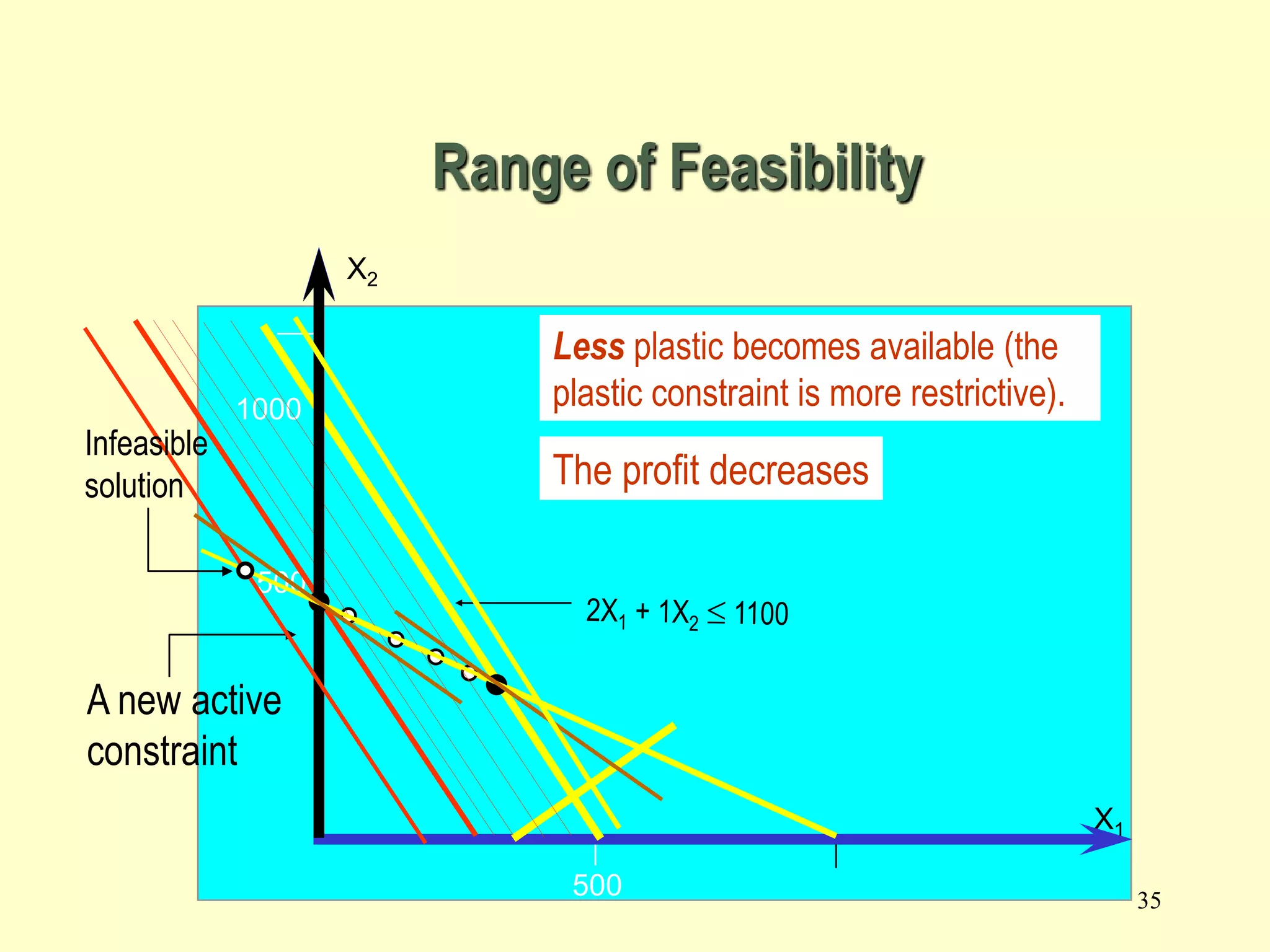
Range of Feasibility
• Assuming there are no other changes to the
input parameters, the range of feasibility is
– The range of values for a right hand side of a constraint, in
which the shadow prices for the constraints remain
unchanged.
– In the range of feasibility the objective function value changes
as follows:
Change in objective value =
[Shadow price][Change in the right hand side value]

33. 33
Range of Feasibility
1000
500
X2
X1
500
Increasing the amount of
plastic is only effective until a
new constraint becomes active.
The Plastic
constraint
This is an infeasible solution
Production time
constraint
Production mix
constraint
X1 + X2 700
A new active
constraint

34. 34
Range of Feasibility
1000
500
X2
X1
500
The Plastic
constraint
Production time
constraint
Note how the profit increases
as the amount of plastic
increases.

35. 35
Range of Feasibility
1000
500
X2
X1
500
Less plastic becomes available (the
plastic constraint is more restrictive).
The profit decreases
A new active
constraint
Infeasible
solution

36. 36
– Sunk costs: The shadow price is the value of an
extra unit of the resource, since the cost of the
resource is not included in the calculation of the
objective function coefficient.
– Included costs: The shadow price is the premium
value above the existing unit value for the resource,
since the cost of the resource is included in the
calculation of the objective function coefficient.
The correct interpretation of shadow prices

37. 37
Other Post - Optimality Changes
• Addition of a constraint.
• Deletion of a constraint.
• Addition of a variable.
• Deletion of a variable.
• Changes in the left - hand side coefficients.

38. 38
2.5 Using Excel Solver to Find an
Optimal Solution and Analyze Results
• To see the input screen in Excel click Galaxy.xls
• Click Solver to obtain the following dialog box.
Equal To:
By Changing cells
These cells contain
the decision variables
$B$4:$C$4
To enter constraints click…
Set Target cell $D$6
This cell contains
the value of the
objective function
$D$7:$D$10 $F$7:$F$10
All the constraints
have the same direction,
thus are included in
one “Excel constraint”.

39. 39
Using Excel Solver
• To see the input screen in Excel click Galaxy.xls
• Click Solver to obtain the following dialog box.
Equal To:
$D$7:$D$10<=$F$7:$F$10
By Changing cells
These cells contain
the decision variables
$B$4:$C$4
Set Target cell $D$6
This cell contains
the value of the
objective function
Click on ‘Options’
and check ‘Linear
Programming’ and
‘Non-negative’.

40. 40
• To see the input screen in Excel click Galaxy.xls
• Click Solver to obtain the following dialog box.
Equal To:
$D$7:$D$10<=$F$7:$F$10
By Changing cells
$B$4:$C$4
Set Target cell $D$6
Using Excel Solver

41. 41
Space Rays Zappers
Dozens 320 360
Total Limit
Profit 8 5 4360
Plastic 2 1 1000 <= 1000
Prod. Time 3 4 2400 <= 2400
Total 1 1 680 <= 700
Mix 1 -1 -40 <= 350
GALAXY INDUSTRIES
Using Excel Solver – Optimal Solution

42. 42
Space Rays Zappers
Dozens 320 360
Total Limit
Profit 8 5 4360
Plastic 2 1 1000 <= 1000
Prod. Time 3 4 2400 <= 2400
Total 1 1 680 <= 700
Mix 1 -1 -40 <= 350
GALAXY INDUSTRIES
Using Excel Solver – Optimal Solution
Solver is ready to provide
reports to analyze the
optimal solution.

43. 43
Using Excel Solver –Answer Report
Microsoft Excel 9.0 Answer Report
Worksheet: [Galaxy.xls]Galaxy
Report Created: 11/12/2001 8:02:06 PM
Target Cell (Max)
Cell Name Original Value Final Value
$D$6 Profit Total 4360 4360
Adjustable Cells
Cell Name Original Value Final Value
$B$4 Dozens Space Rays 320 320
$C$4 Dozens Zappers 360 360
Constraints
Cell Name Cell Value Formula Status Slack
$D$7 Plastic Total 1000 $D$7<=$F$7 Binding 0
$D$8 Prod. Time Total 2400 $D$8<=$F$8 Binding 0
$D$9 Total Total 680 $D$9<=$F$9 Not Binding 20
$D$10 Mix Total -40 $D$10<=$F$10 Not Binding 390

44. 44
Using Excel Solver –Sensitivity
Report
Microsoft Excel Sensitivity Report
Worksheet: [Galaxy.xls]Sheet1
Report Created:
Adjustable Cells
Final Reduced Objective Allowable Allowable
Cell Name Value Cost Coefficient Increase Decrease
$B$4 Dozens Space Rays 320 0 8 2 4.25
$C$4 Dozens Zappers 360 0 5 5.666666667 1
Constraints
Final Shadow Constraint Allowable Allowable
Cell Name Value Price R.H. Side Increase Decrease
$D$7 Plastic Total 1000 3.4 1000 100 400
$D$8 Prod. Time Total 2400 0.4 2400 100 650
$D$9 Total Total 680 0 700 1E+30 20
$D$10 Mix Total -40 0 350 1E+30 390

45. 45
• Infeasibility: Occurs when a model has no feasible
point.
• Unboundness: Occurs when the objective can become
infinitely large (max), or infinitely small (min).
• Alternate solution: Occurs when more than one point
optimizes the objective function
2.7 Models Without Unique Optimal
Solutions

46. 46
1
No point, simultaneously,
lies both above line and
below lines and
.
1
2 3
2
3
Infeasible Model

47. 47
Solver – Infeasible Model

48. 48
Unbounded solution


49. 49
Solver – Unbounded solution

50. 50
• Solver does not alert the user to the existence of
alternate optimal solutions.
• Many times alternate optimal solutions exist
when the allowable increase or allowable
decrease is equal to zero.
• In these cases, we can find alternate optimal
solutions using Solver by the following procedure:
Solver – An Alternate Optimal Solution

51. 51
• Observe that for some variable Xj the
Allowable increase = 0, or
Allowable decrease = 0.
• Add a constraint of the form:
Objective function = Current optimal value.
• If Allowable increase = 0, change the objective to
Maximize Xj
• If Allowable decrease = 0, change the objective to
Minimize Xj
Solver – An Alternate Optimal Solution

52. 52
2.8 Cost Minimization Diet Problem
• Mix two sea ration products: Texfoods, Calration.
• Minimize the total cost of the mix.
• Meet the minimum requirements of Vitamin A,
Vitamin D, and Iron.

53. 53
• Decision variables
– X1 (X2) -- The number of two-ounce portions of
Texfoods (Calration) product used in a serving.
• The Model
Minimize 0.60X1 + 0.50X2
Subject to
20X1 + 50X2  100 Vitamin A
25X1 + 25X2  100 Vitamin D
50X1 + 10X2  100 Iron
X1, X2  0
Cost per 2 oz.
% Vitamin A
provided per 2 oz.
% required
Cost Minimization Diet Problem

54. 54
10
2 4 5
Feasible Region
Vitamin “D” constraint
Vitamin “A” constraint
The Iron constraint
The Diet Problem - Graphical solution

55. 55
• Summary of the optimal solution
– Texfood product = 1.5 portions (= 3 ounces)
Calration product = 2.5 portions (= 5 ounces)
– Cost =$ 2.15 per serving.
– The minimum requirement for Vitamin D and iron are met with
no surplus.
– The mixture provides 155% of the requirement for Vitamin A.
Cost Minimization Diet Problem

56. 56
• Linear programming software packages solve
large linear models.
• Most of the software packages use the algebraic
technique called the Simplex algorithm.
• The input to any package includes:
– The objective function criterion (Max or Min).
– The type of each constraint: .
– The actual coefficients for the problem.
Computer Solution of Linear Programs With
Any Number of Decision Variables
  
, ,