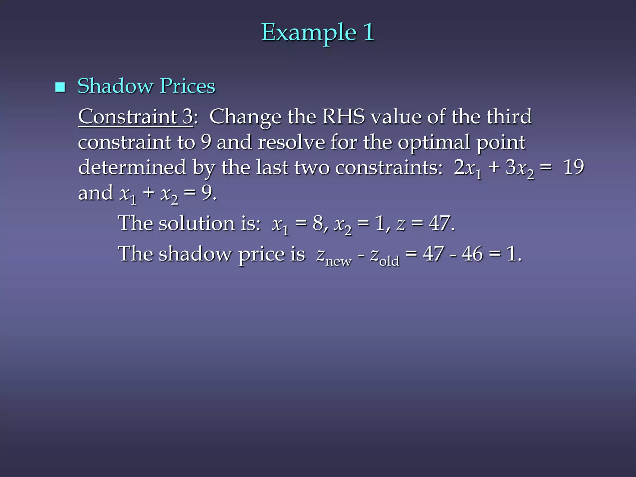
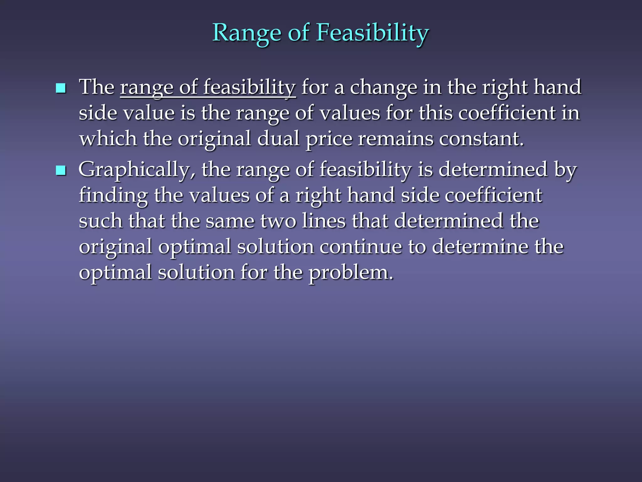
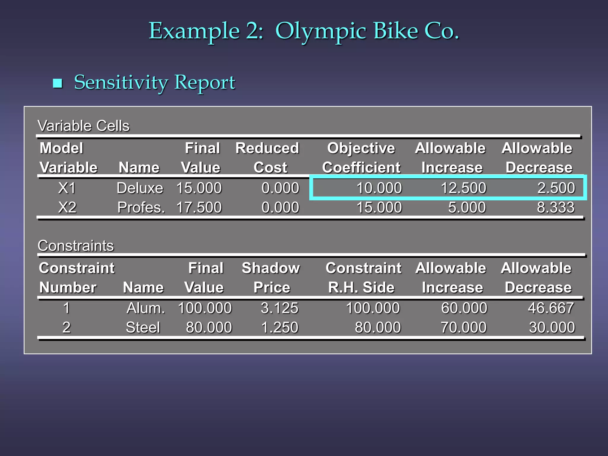
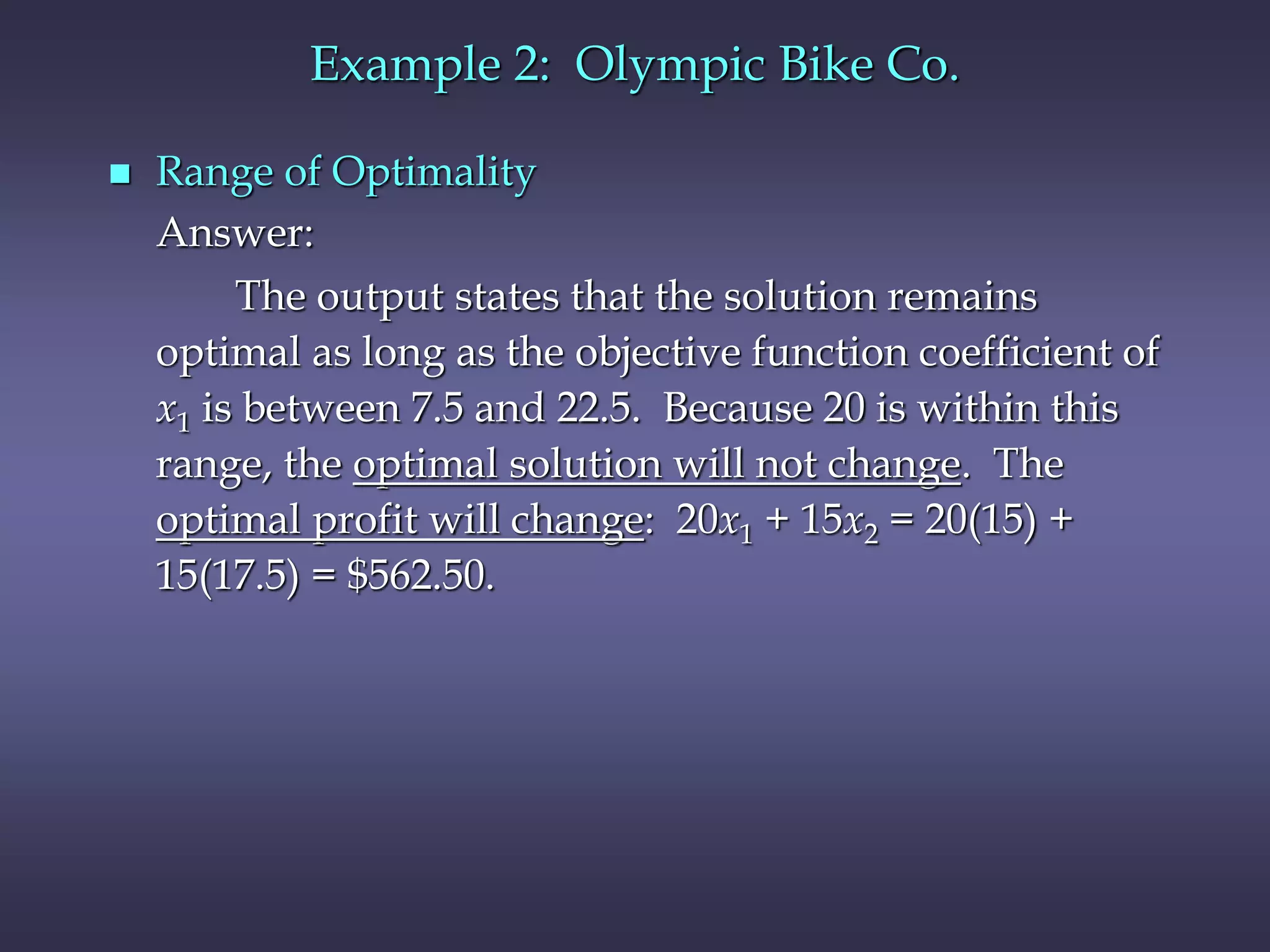
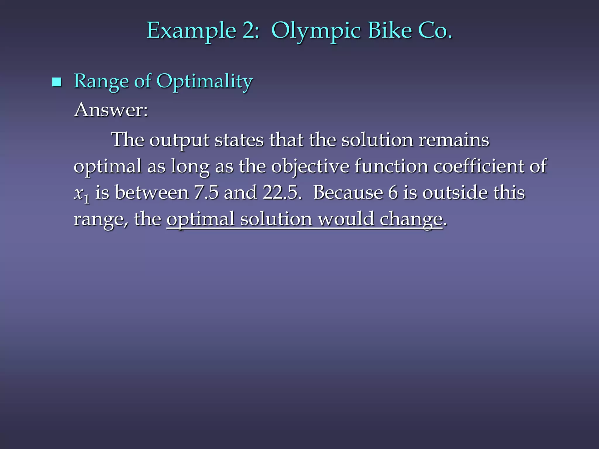
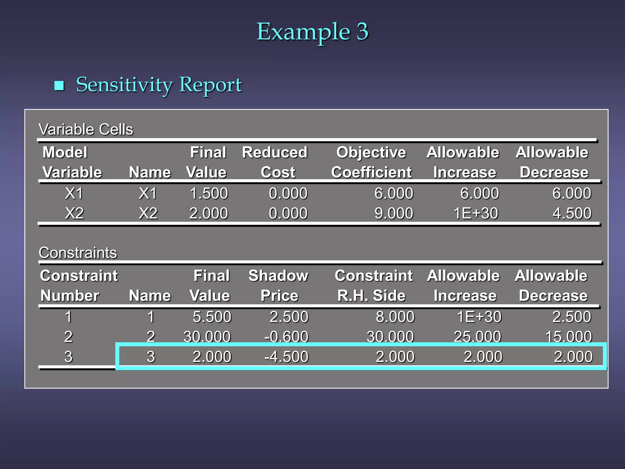
Chapter 8
Linear Programming: Sensitivity Analysis
and Interpretation of Solution
 Introduction to Sensitivity Analysis
 Objective Function Coefficients
 Right-Hand Sides
 Limitations of Classical Sensitivity Analysis
 In the previous chapter we discussed:
•objective function value
•values of the decision variables
•reduced costs
•slack/surplus
 In this chapter we will discuss:
•changes in the coefficients of the objective function
•changes in the right-hand side value of a
constraint
Introduction to Sensitivity Analysis
 Sensitivity analysis (or post-optimality analysis) is
used to determine how the optimal solution is
affected by changes, within specified ranges, in:
•the objective function coefficients
•the right-hand side (RHS) values
 Sensitivity analysis is important to a manager who
must operate in a dynamic environment with
imprecise estimates of the coefficients.
 Sensitivity analysis allows a manager to ask certain
what-if questions about the problem.
Example 1
 LP Formulation
Max 5x1 + 7x2
s.t. x1 < 6
2x1 + 3x2 < 19
x1 + x2 < 8
x1, x2 > 0
Example 1
 Graphical Solution
2x1 + 3x2 < 19
x2
x1
x1 + x2 < 8
Max 5x1 + 7x2
x1 < 6
Optimal Solution:
x1 = 5, x2 = 3
8
7
6
5
4
3
2
1
1 2 3 4 5 6 7 8 9 10
Objective Function Coefficients
 Let us consider how changes in the objective function
coefficients might affect the optimal solution.
 The range of optimality for each coefficient provides
the range of values over which the current solution
will remain optimal.
 Managers should focus on those objective coefficients
that have a narrow range of optimality and
coefficients near the endpoints of the range.
Example 1
 Changing Slope of Objective Function
x1
Feasible
Region
1 2
3
4
5
x2
Coincides with
x1 + x2 < 8
constraint line
8
7
6
5
4
3
2
1
1 2 3 4 5 6 7 8 9 10
Coincides with
2x1 + 3x2 < 19
constraint line
Objective function
line for 5x1 + 7x2
Range of Optimality
 Graphically, the limits of a range of optimality are
found by changing the slope of the objective function
line within the limits of the slopes of the binding
constraint lines.
 Slope of an objective function line, Max c1x1 + c2x2, is
-c1/c2, and the slope of a constraint, a1x1 + a2x2 = b, is
-a1/a2.
Example 1
 Range of Optimality for c1
The slope of the objective function line is -c1/c2.
The slope of the first binding constraint, x1 + x2 = 8, is
-1 and the slope of the second binding constraint,
x1 + 3x2 = 19, is -2/3.
Find the range of values for c1 (with c2 staying 7)
such that the objective function line slope lies between
that of the two binding constraints:
-1 < -c1/7 < -2/3
Multiplying through by -7 (and reversing the
inequalities):
14/3 < c1 < 7
Example 1
 Range of Optimality for c2
Find the range of values for c2 ( with c1 staying 5)
such that the objective function line slope lies between
that of the two binding constraints:
-1 < -5/c2 < -2/3
Multiplying by -1: 1 > 5/c2 > 2/3
Inverting, 1 < c2/5 < 3/2
Multiplying by 5: 5 < c2 < 15/2
Software packages such as LINGO and Microsoft Excel
provide the following LP information:
 Information about the objective function:
•its optimal value
•coefficient ranges (ranges of optimality)
 Information about the decision variables:
•their optimal values
•their reduced costs
 Information about the constraints:
•the amount of slack or surplus
•the dual prices
•right-hand side ranges (ranges of feasibility)
Sensitivity Analysis: Computer Solution
Example 1
 Range of Optimality for c1 and c2
Variable Cells
Final Reduced Objective Allowable Allowable
Name Value Cost Coefficient Increase Decrease
X1 5.000 0.000 5.000 2.000 0.333
X2 3.000 0.000 7.000 0.500 2.000
Constraints
Final Shadow Constraint Allowable Allowable
Name Value Price R.H. Side Increase Decrease
1 5.000 0.000 6.000 1E+30 1.000
2 19.000 2.000 19.000 5.000 1.000
3 8.000 1.000 8.000 0.333 1.667
Variable
Model
X1
X2
1
2
3
Number
Constraint
Right-Hand Sides
 Let us consider how a change in the right-hand side
for a constraint might affect the feasible region and
perhaps cause a change in the optimal solution.
 The improvement in the value of the optimal solution
per unit increase in the right-hand side is called the
shadow price.
 The range of feasibility is the range over which the
shadow price is applicable.
 As the RHS increases, other constraints will become
binding and limit the change in the value of the
objective function.
Shadow Price
 Graphically, a shadow price is determined by adding
+1 to the right hand side value in question and then
resolving for the optimal solution in terms of the
same two binding constraints.
 The shadow price for a nonbinding constraint is 0.
 A negative shadow price indicates that the objective
function will not improve if the RHS is increased.
Relevant Cost and Sunk Cost
 A resource cost is a relevant cost if the amount paid
for it is dependent upon the amount of the resource
used by the decision variables.
 Relevant costs are reflected in the objective function
coefficients.
 A resource cost is a sunk cost if it must be paid
regardless of the amount of the resource actually used
by the decision variables.
 Sunk resource costs are not reflected in the objective
function coefficients.
Cautionary Note on the
Interpretation of Shadow Prices
 Resource Cost is Sunk
The shadow price is the maximum amount you
should be willing to pay for one additional unit of the
resource.
 Resource Cost is Relevant
The shadow price is the maximum premium over the
normal cost that you should be willing to pay for one
unit of the resource.
Example 1
 Shadow Prices
Constraint 1: Since x1 < 6 is not a binding constraint,
its shadow price is 0.
Constraint 2: Change the RHS value of the second
constraint to 20 and resolve for the optimal point
determined by the last two constraints:
2x1 + 3x2 = 20 and x1 + x2 = 8.
The solution is x1 = 4, x2 = 4, z = 48. Hence,
the shadow price = znew - zold = 48 - 46 = 2.
Example 1
 Shadow Prices
Constraint 3: Change the RHS value of the third
constraint to 9 and resolve for the optimal point
determined by the last two constraints: 2x1 + 3x2 = 19
and x1 + x2 = 9.
The solution is: x1 = 8, x2 = 1, z = 47.
The shadow price is znew - zold = 47 - 46 = 1.
Example 1
 Shadow Prices
Variable Cells
Final Reduced Objective Allowable Allowable
Name Value Cost Coefficient Increase Decrease
X1 5.000 0.000 5.000 2.000 0.333
X2 3.000 0.000 7.000 0.500 2.000
Constraints
Final Shadow Constraint Allowable Allowable
Name Value Price R.H. Side Increase Decrease
1 5.000 0.000 6.000 1E+30 1.000
2 19.000 2.000 19.000 5.000 1.000
3 8.000 1.000 8.000 0.333 1.667
Variable
Model
X1
X2
1
2
3
Number
Constraint
Range of Feasibility
 The range of feasibility for a change in the right hand
side value is the range of values for this coefficient in
which the original dual price remains constant.
 Graphically, the range of feasibility is determined by
finding the values of a right hand side coefficient
such that the same two lines that determined the
original optimal solution continue to determine the
optimal solution for the problem.
Example 1
 Range of Feasibility
Variable Cells
Final Reduced Objective Allowable Allowable
Name Value Cost Coefficient Increase Decrease
X1 5.000 0.000 5.000 2.000 0.333
X2 3.000 0.000 7.000 0.500 2.000
Constraints
Final Shadow Constraint Allowable Allowable
Name Value Price R.H. Side Increase Decrease
1 5.000 0.000 6.000 1E+30 1.000
2 19.000 2.000 19.000 5.000 1.000
3 8.000 1.000 8.000 0.333 1.667
Variable
Model
X1
X2
1
2
3
Number
Constraint
Olympic Bike is introducing two new lightweight
bicycle frames, the Deluxe and the Professional, to be
made from special aluminum and steel alloys. The
anticipated unit profits are $10 for the Deluxe and $15 for
the Professional. The number of pounds of each alloy
needed per frame is summarized on the next slide.
Example 2: Olympic Bike Co.
A supplier delivers 100 pounds of the
aluminum alloy and 80 pounds of the steel
alloy weekly.
Aluminum Alloy Steel Alloy
Deluxe 2 3
Professional 4 2
How many Deluxe and Professional frames should
Olympic produce each week?
Example 2: Olympic Bike Co.
 Model Formulation
•Verbal Statement of the Objective Function
Maximize total weekly profit.
•Verbal Statement of the Constraints
Total weekly usage of aluminum alloy < 100 pounds.
Total weekly usage of steel alloy < 80 pounds.
•Definition of the Decision Variables
x1 = number of Deluxe frames produced weekly.
x2 = number of Professional frames produced weekly.
Example 2: Olympic Bike Co.
 Model Formulation (continued)
Max 10x1 + 15x2 (Total Weekly Profit)
s.t. 2x1 + 4x2 < 100 (Aluminum Available)
3x1 + 2x2 < 80 (Steel Available)
x1, x2 > 0
Example 2: Olympic Bike Co.
 Partial Spreadsheet Showing Solution
A B C D
6
7 Deluxe Professional
8 Bikes Made 15 17.500
9
10 412.500
11
12 Constraints Amount Used Amount Avail.
13 Aluminum 100 <= 100
14 Steel 80 <= 80
Decision Variables
Maximized Total Profit
A B C D
6
7 Deluxe Professional
8 Bikes Made 15 17.500
9
10 412.500
11
12 Constraints Amount Used Amount Avail.
13 Aluminum 100 <= 100
14 Steel 80 <= 80
Decision Variables
Maximized Total Profit
Example 2: Olympic Bike Co.
 Optimal Solution
According to the output:
x1 (Deluxe frames) = 15
x2 (Professional frames) = 17.5
Objective function value = $412.50
Example 2: Olympic Bike Co.
 Range of Optimality
Question:
Suppose the profit on deluxe frames is increased
to $20. Is the above solution still optimal? What is
the value of the objective function when this unit
profit is increased to $20?
Example 2: Olympic Bike Co.
 Sensitivity Report
Variable Cells
Final Reduced Objective Allowable Allowable
Name Value Cost Coefficient Increase Decrease
Deluxe 15.000 0.000 10.000 12.500 2.500
Profes. 17.500 0.000 15.000 5.000 8.333
Constraints
Final Shadow Constraint Allowable Allowable
Name Value Price R.H. Side Increase Decrease
Alum. 100.000 3.125 100.000 60.000 46.667
Steel 80.000 1.250 80.000 70.000 30.000
Variable
Model
X1
X2
1
2
Number
Constraint
Example 2: Olympic Bike Co.
 Range of Optimality
Answer:
The output states that the solution remains
optimal as long as the objective function coefficient of
x1 is between 7.5 and 22.5. Because 20 is within this
range, the optimal solution will not change. The
optimal profit will change: 20x1 + 15x2 = 20(15) +
15(17.5) = $562.50.
Example 2: Olympic Bike Co.
 Range of Optimality
Question:
If the unit profit on deluxe frames were $6
instead of $10, would the optimal solution change?
Example 2: Olympic Bike Co.
 Range of Optimality
Variable Cells
Final Reduced Objective Allowable Allowable
Name Value Cost Coefficient Increase Decrease
Deluxe 15.000 0.000 10.000 12.500 2.500
Profes. 17.500 0.000 15.000 5.000 8.333
Constraints
Final Shadow Constraint Allowable Allowable
Name Value Price R.H. Side Increase Decrease
Alum. 100.000 3.125 100.000 60.000 46.667
Steel 80.000 1.250 80.000 70.000 30.000
Variable
Model
X1
X2
1
2
Number
Constraint
 Range of Optimality
Answer:
The output states that the solution remains
optimal as long as the objective function coefficient of
x1 is between 7.5 and 22.5. Because 6 is outside this
range, the optimal solution would change.
Example 2: Olympic Bike Co.
Simultaneous Changes
 Range of Optimality and 100% Rule
The 100% rule states that simultaneous changes in
objective function coefficients will not change the
optimal solution as long as the sum of the percentages
of the change divided by the corresponding maximum
allowable change in the range of optimality for each
coefficient does not exceed 100%.
Example 2: Olympic Bike Co.
 Range of Optimality and 100% Rule
Question:
If simultaneously the profit on Deluxe frames
was raised to $16 and the profit on Professional
frames was raised to $17, would the current solution
be optimal?
Example 2: Olympic Bike Co.
 Range of Optimality and 100% Rule
Answer:
If c1 = 16, the amount c1 changed is 16 - 10 = 6 .
The maximum allowable increase is 22.5 - 10 = 12.5,
so this is a 6/12.5 = 48% change. If c2 = 17, the
amount that c2 changed is 17 - 15 = 2. The maximum
allowable increase is 20 - 15 = 5 so this is a 2/5 = 40%
change. The sum of the change percentages is 88%.
Since this does not exceed 100%, the optimal solution
would not change.
Simultaneous Changes
 Range of Feasibility and 100% Rule
The 100% rule states that simultaneous changes in
right-hand sides will not change the dual prices as
long as the sum of the percentages of the changes
divided by the corresponding maximum allowable
change in the range of feasibility for each right-hand
side does not exceed 100%.
Example 2: Olympic Bike Co.
 Range of Feasibility and Sunk Costs
Question:
Given that aluminum is a sunk cost, what is the
maximum amount the company should pay for 50
extra pounds of aluminum?
Example 2: Olympic Bike Co.
 Range of Feasibility and Sunk Costs
Variable Cells
Final Reduced Objective Allowable Allowable
Name Value Cost Coefficient Increase Decrease
Deluxe 15.000 0.000 10.000 12.500 2.500
Profes. 17.500 0.000 15.000 5.000 8.333
Constraints
Final Shadow Constraint Allowable Allowable
Name Value Price R.H. Side Increase Decrease
Alum. 100.000 3.125 100.000 60.000 46.667
Steel 80.000 1.250 80.000 70.000 30.000
Variable
Model
X1
X2
1
2
Number
Constraint
Example 2: Olympic Bike Co.
 Range of Feasibility and Sunk Costs
Answer:
Because the cost for aluminum is a sunk cost, the
shadow price provides the value of extra aluminum.
The shadow price for aluminum is $3.125 per pound
and the maximum allowable increase is 60 pounds.
Because 50 is in this range, the $3.125 is valid. Thus,
the value of 50 additional pounds is = 50($3.125) =
$156.25.
Example 2: Olympic Bike Co.
 Range of Feasibility and Relevant Costs
Question:
If aluminum were a relevant cost, what is the
maximum amount the company should pay for 50
extra pounds of aluminum?
Example 2: Olympic Bike Co.
 Range of Feasibility and Relevant Costs
Answer:
If aluminum were a relevant cost, the shadow
price would be the amount above the normal price of
aluminum the company would be willing to pay.
Thus if initially aluminum cost $4 per pound, then
additional units in the range of feasibility would be
worth $4 + $3.125 = $7.125 per pound.
Example 3
 Consider the following linear program:
Min 6x1 + 9x2 ($ cost)
s.t. x1 + 2x2 < 8
10x1 + 7.5x2 > 30
x2 > 2
x1, x2 > 0
Variable Cells
Final Reduced Objective Allowable Allowable
Name Value Cost Coefficient Increase Decrease
X1 1.500 0.000 6.000 6.000 6.000
X2 2.000 0.000 9.000 1E+30 4.500
Constraints
Final Shadow Constraint Allowable Allowable
Name Value Price R.H. Side Increase Decrease
1 5.500 2.500 8.000 1E+30 2.500
2 30.000 -0.600 30.000 25.000 15.000
3 2.000 -4.500 2.000 2.000 2.000
Variable
Model
X1
X2
1
2
3
Number
Constraint
Example 3
 Sensitivity Report
Example 3
 Optimal Solution
According to the output:
x1 = 1.5
x2 = 2.0
Objective function value = 27.00
Example 3
 Range of Optimality
Question:
Suppose the unit cost of x1 is decreased to $4. Is
the current solution still optimal? What is the value
of the objective function when this unit cost is
decreased to $4?
Example 3
Variable Cells
Final Reduced Objective Allowable Allowable
Name Value Cost Coefficient Increase Decrease
X1 1.500 0.000 6.000 6.000 6.000
X2 2.000 0.000 9.000 1E+30 4.500
Constraints
Final Shadow Constraint Allowable Allowable
Name Value Price R.H. Side Increase Decrease
1 5.500 2.500 8.000 1E+30 2.500
2 30.000 -0.600 30.000 25.000 15.000
3 2.000 -4.500 2.000 2.000 2.000
Variable
Model
X1
X2
1
2
3
Number
Constraint
 Sensitivity Report
Example 3
 Range of Optimality
Answer:
The output states that the solution remains
optimal as long as the objective function coefficient of
x1 is between 0 and 12. Because 4 is within this range,
the optimal solution will not change. However, the
optimal total cost will change: 6x1 + 9x2 = 4(1.5) +
9(2.0) = $24.00.
Example 3
 Range of Optimality
Question:
How much can the unit cost of x2 be decreased
without concern for the optimal solution changing?
Example 3
Variable Cells
Final Reduced Objective Allowable Allowable
Name Value Cost Coefficient Increase Decrease
X1 1.500 0.000 6.000 6.000 6.000
X2 2.000 0.000 9.000 1E+30 4.500
Constraints
Final Shadow Constraint Allowable Allowable
Name Value Price R.H. Side Increase Decrease
1 5.500 2.500 8.000 1E+30 2.500
2 30.000 -0.600 30.000 25.000 15.000
3 2.000 -4.500 2.000 2.000 2.000
Variable
Model
X1
X2
1
2
3
Number
Constraint
 Sensitivity Report
Example 3
 Range of Optimality
Answer:
The output states that the solution remains
optimal as long as the objective function coefficient of
x2 does not fall below 4.5.
Example 3
 Range of Optimality and 100% Rule
Question:
If simultaneously the cost of x1 was raised to $7.5
and the cost of x2 was reduced to $6, would the current
solution remain optimal?
Example 3
Variable Cells
Final Reduced Objective Allowable Allowable
Name Value Cost Coefficient Increase Decrease
X1 1.500 0.000 6.000 6.000 6.000
X2 2.000 0.000 9.000 1E+30 4.500
Constraints
Final Shadow Constraint Allowable Allowable
Name Value Price R.H. Side Increase Decrease
1 5.500 2.500 8.000 1E+30 2.500
2 30.000 -0.600 30.000 25.000 15.000
3 2.000 -4.500 2.000 2.000 2.000
Variable
Model
X1
X2
1
2
3
Number
Constraint
 Sensitivity Report
Example 3
 Range of Optimality and 100% Rule
Answer:
If c1 = 7.5, the amount c1 changed is 7.5 - 6 = 1.5.
The maximum allowable increase is 12 - 6 = 6, so this
is a 1.5/6 = 25% change. If c2 = 6, the amount that c2
changed is 9 - 6 = 3. The maximum allowable
decrease is 9 - 4.5 = 4.5, so this is a 3/4.5 = 66.7%
change. The sum of the change percentages is 25% +
66.7% = 91.7%. Because this does not exceed 100%,
the optimal solution would not change.
Example 3
 Range of Feasibility
Question:
If the right-hand side of constraint 3 is increased
by 1, what will be the effect on the optimal solution?
Example 3
Variable Cells
Final Reduced Objective Allowable Allowable
Name Value Cost Coefficient Increase Decrease
X1 1.500 0.000 6.000 6.000 6.000
X2 2.000 0.000 9.000 1E+30 4.500
Constraints
Final Shadow Constraint Allowable Allowable
Name Value Price R.H. Side Increase Decrease
1 5.500 2.500 8.000 1E+30 2.500
2 30.000 -0.600 30.000 25.000 15.000
3 2.000 -4.500 2.000 2.000 2.000
Variable
Model
X1
X2
1
2
3
Number
Constraint
 Sensitivity Report
Example 3
 Range of Feasibility
Answer:
A shadow price represents the improvement in
the objective function value per unit increase in the
right-hand side. A negative shadow price indicates a
deterioration (negative improvement) in the
objective, which in this problem means an increase in
total cost because we're minimizing. Since the right-
hand side remains within the range of feasibility,
there is no change in the optimal solution. However,
the objective function value increases by $4.50.
Changes in Constraint Coefficients
 Classical sensitivity analysis provides no information
about changes resulting from a change in the
coefficient of a variable in a constraint.
 We must change the coefficient and rerun the model
to learn the impact the change will have on the
solution.
Non-intuitive Shadow Prices
 Constraints with variables naturally on both the left-
hand and right-hand sides often lead to shadow
prices that have a non-intuitive explanation.
Example 2: Olympic Bike Co. (Revised)
Recall that Olympic Bike is introducing two new
lightweight bicycle frames, the Deluxe and the
Professional, to be made from special aluminum and
steel alloys. The objective is to maximize total profit,
subject to limits on the availability of aluminum and
steel.
Let us now introduce an additional constraint. The
number of Deluxe frames produced (x1) must be greater
than or equal to the number of Professional frames
produced (x2) .
x1 > x2
Example 2: Olympic Bike Co. (Revised)
 Model Formulation (continued)
Max 10x1 + 15x2 (Total Weekly Profit)
s.t. 2x1 + 4x2 < 100 (Aluminum Available)
3x1 + 2x2 < 80 (Steel Available)
x1 - x2 > 0 (Product Ratio)
x1, x2 > 0
Variable Cells
Final Reduced Objective Allowable Allowable
Name Value Cost Coefficient Increase Decrease
Deluxe 16.000 0.000 10.000 12.500 10.000
Profes. 16.000 0.000 15.000 1E+30 8.333
Constraints
Final Shadow Constraint Allowable Allowable
Name Value Price R.H. Side Increase Decrease
Alum. 96.000 0.000 100.000 1E+30 4.000
Steel 80.000 5.000 80.000 3.333 80.000
Variable
Model
X1
X2
1
2
Number
Constraint
Example 2: Olympic Bike Co. (Revised)
 Sensitivity Report (Revised)
Ratio 0.000 -5.000 0.000 26.667 2.500
3
Example 2: Olympic Bike Co. (Revised)
 Shadow Price for Constraint #3
The interpretation of the shadow price -5.00 is
correctly stated as follows:
“If we are forced to produce 1 more Deluxe frame
over and above the number of Professional frames
produced, total profits will decrease by $5.00.”
Example 2: Olympic Bike Co. (Revised Again)
We might instead be interested in what happens if
we change the coefficient on x2.
For instance, what if management required Olympic
to produce a number of Deluxe frames that is at least
110% of the number of Professional frames produced?
In other words, the constraint would change to
x1 > 1.1x2
The shadow price does not tell us what will happen
in this case. We need to resolve the problem with this
new constraint.
End of Chapter 8

qmb12ch08.pptx

  • 1.
    Chapter 8 Linear Programming:Sensitivity Analysis and Interpretation of Solution  Introduction to Sensitivity Analysis  Objective Function Coefficients  Right-Hand Sides  Limitations of Classical Sensitivity Analysis
  • 2.
     In theprevious chapter we discussed: •objective function value •values of the decision variables •reduced costs •slack/surplus  In this chapter we will discuss: •changes in the coefficients of the objective function •changes in the right-hand side value of a constraint Introduction to Sensitivity Analysis
  • 3.
    Introduction to SensitivityAnalysis  Sensitivity analysis (or post-optimality analysis) is used to determine how the optimal solution is affected by changes, within specified ranges, in: •the objective function coefficients •the right-hand side (RHS) values  Sensitivity analysis is important to a manager who must operate in a dynamic environment with imprecise estimates of the coefficients.  Sensitivity analysis allows a manager to ask certain what-if questions about the problem.
  • 4.
    Example 1  LPFormulation Max 5x1 + 7x2 s.t. x1 < 6 2x1 + 3x2 < 19 x1 + x2 < 8 x1, x2 > 0
  • 5.
    Example 1  GraphicalSolution 2x1 + 3x2 < 19 x2 x1 x1 + x2 < 8 Max 5x1 + 7x2 x1 < 6 Optimal Solution: x1 = 5, x2 = 3 8 7 6 5 4 3 2 1 1 2 3 4 5 6 7 8 9 10
  • 6.
    Objective Function Coefficients Let us consider how changes in the objective function coefficients might affect the optimal solution.  The range of optimality for each coefficient provides the range of values over which the current solution will remain optimal.  Managers should focus on those objective coefficients that have a narrow range of optimality and coefficients near the endpoints of the range.
  • 7.
    Example 1  ChangingSlope of Objective Function x1 Feasible Region 1 2 3 4 5 x2 Coincides with x1 + x2 < 8 constraint line 8 7 6 5 4 3 2 1 1 2 3 4 5 6 7 8 9 10 Coincides with 2x1 + 3x2 < 19 constraint line Objective function line for 5x1 + 7x2
  • 8.
    Range of Optimality Graphically, the limits of a range of optimality are found by changing the slope of the objective function line within the limits of the slopes of the binding constraint lines.  Slope of an objective function line, Max c1x1 + c2x2, is -c1/c2, and the slope of a constraint, a1x1 + a2x2 = b, is -a1/a2.
  • 9.
    Example 1  Rangeof Optimality for c1 The slope of the objective function line is -c1/c2. The slope of the first binding constraint, x1 + x2 = 8, is -1 and the slope of the second binding constraint, x1 + 3x2 = 19, is -2/3. Find the range of values for c1 (with c2 staying 7) such that the objective function line slope lies between that of the two binding constraints: -1 < -c1/7 < -2/3 Multiplying through by -7 (and reversing the inequalities): 14/3 < c1 < 7
  • 10.
    Example 1  Rangeof Optimality for c2 Find the range of values for c2 ( with c1 staying 5) such that the objective function line slope lies between that of the two binding constraints: -1 < -5/c2 < -2/3 Multiplying by -1: 1 > 5/c2 > 2/3 Inverting, 1 < c2/5 < 3/2 Multiplying by 5: 5 < c2 < 15/2
  • 11.
    Software packages suchas LINGO and Microsoft Excel provide the following LP information:  Information about the objective function: •its optimal value •coefficient ranges (ranges of optimality)  Information about the decision variables: •their optimal values •their reduced costs  Information about the constraints: •the amount of slack or surplus •the dual prices •right-hand side ranges (ranges of feasibility) Sensitivity Analysis: Computer Solution
  • 12.
    Example 1  Rangeof Optimality for c1 and c2 Variable Cells Final Reduced Objective Allowable Allowable Name Value Cost Coefficient Increase Decrease X1 5.000 0.000 5.000 2.000 0.333 X2 3.000 0.000 7.000 0.500 2.000 Constraints Final Shadow Constraint Allowable Allowable Name Value Price R.H. Side Increase Decrease 1 5.000 0.000 6.000 1E+30 1.000 2 19.000 2.000 19.000 5.000 1.000 3 8.000 1.000 8.000 0.333 1.667 Variable Model X1 X2 1 2 3 Number Constraint
  • 13.
    Right-Hand Sides  Letus consider how a change in the right-hand side for a constraint might affect the feasible region and perhaps cause a change in the optimal solution.  The improvement in the value of the optimal solution per unit increase in the right-hand side is called the shadow price.  The range of feasibility is the range over which the shadow price is applicable.  As the RHS increases, other constraints will become binding and limit the change in the value of the objective function.
  • 14.
    Shadow Price  Graphically,a shadow price is determined by adding +1 to the right hand side value in question and then resolving for the optimal solution in terms of the same two binding constraints.  The shadow price for a nonbinding constraint is 0.  A negative shadow price indicates that the objective function will not improve if the RHS is increased.
  • 15.
    Relevant Cost andSunk Cost  A resource cost is a relevant cost if the amount paid for it is dependent upon the amount of the resource used by the decision variables.  Relevant costs are reflected in the objective function coefficients.  A resource cost is a sunk cost if it must be paid regardless of the amount of the resource actually used by the decision variables.  Sunk resource costs are not reflected in the objective function coefficients.
  • 16.
    Cautionary Note onthe Interpretation of Shadow Prices  Resource Cost is Sunk The shadow price is the maximum amount you should be willing to pay for one additional unit of the resource.  Resource Cost is Relevant The shadow price is the maximum premium over the normal cost that you should be willing to pay for one unit of the resource.
  • 17.
    Example 1  ShadowPrices Constraint 1: Since x1 < 6 is not a binding constraint, its shadow price is 0. Constraint 2: Change the RHS value of the second constraint to 20 and resolve for the optimal point determined by the last two constraints: 2x1 + 3x2 = 20 and x1 + x2 = 8. The solution is x1 = 4, x2 = 4, z = 48. Hence, the shadow price = znew - zold = 48 - 46 = 2.
  • 18.
    Example 1  ShadowPrices Constraint 3: Change the RHS value of the third constraint to 9 and resolve for the optimal point determined by the last two constraints: 2x1 + 3x2 = 19 and x1 + x2 = 9. The solution is: x1 = 8, x2 = 1, z = 47. The shadow price is znew - zold = 47 - 46 = 1.
  • 19.
    Example 1  ShadowPrices Variable Cells Final Reduced Objective Allowable Allowable Name Value Cost Coefficient Increase Decrease X1 5.000 0.000 5.000 2.000 0.333 X2 3.000 0.000 7.000 0.500 2.000 Constraints Final Shadow Constraint Allowable Allowable Name Value Price R.H. Side Increase Decrease 1 5.000 0.000 6.000 1E+30 1.000 2 19.000 2.000 19.000 5.000 1.000 3 8.000 1.000 8.000 0.333 1.667 Variable Model X1 X2 1 2 3 Number Constraint
  • 20.
    Range of Feasibility The range of feasibility for a change in the right hand side value is the range of values for this coefficient in which the original dual price remains constant.  Graphically, the range of feasibility is determined by finding the values of a right hand side coefficient such that the same two lines that determined the original optimal solution continue to determine the optimal solution for the problem.
  • 21.
    Example 1  Rangeof Feasibility Variable Cells Final Reduced Objective Allowable Allowable Name Value Cost Coefficient Increase Decrease X1 5.000 0.000 5.000 2.000 0.333 X2 3.000 0.000 7.000 0.500 2.000 Constraints Final Shadow Constraint Allowable Allowable Name Value Price R.H. Side Increase Decrease 1 5.000 0.000 6.000 1E+30 1.000 2 19.000 2.000 19.000 5.000 1.000 3 8.000 1.000 8.000 0.333 1.667 Variable Model X1 X2 1 2 3 Number Constraint
  • 22.
    Olympic Bike isintroducing two new lightweight bicycle frames, the Deluxe and the Professional, to be made from special aluminum and steel alloys. The anticipated unit profits are $10 for the Deluxe and $15 for the Professional. The number of pounds of each alloy needed per frame is summarized on the next slide. Example 2: Olympic Bike Co.
  • 23.
    A supplier delivers100 pounds of the aluminum alloy and 80 pounds of the steel alloy weekly. Aluminum Alloy Steel Alloy Deluxe 2 3 Professional 4 2 How many Deluxe and Professional frames should Olympic produce each week? Example 2: Olympic Bike Co.
  • 24.
    Example 2: OlympicBike Co.  Model Formulation •Verbal Statement of the Objective Function Maximize total weekly profit. •Verbal Statement of the Constraints Total weekly usage of aluminum alloy < 100 pounds. Total weekly usage of steel alloy < 80 pounds. •Definition of the Decision Variables x1 = number of Deluxe frames produced weekly. x2 = number of Professional frames produced weekly.
  • 25.
    Example 2: OlympicBike Co.  Model Formulation (continued) Max 10x1 + 15x2 (Total Weekly Profit) s.t. 2x1 + 4x2 < 100 (Aluminum Available) 3x1 + 2x2 < 80 (Steel Available) x1, x2 > 0
  • 26.
    Example 2: OlympicBike Co.  Partial Spreadsheet Showing Solution A B C D 6 7 Deluxe Professional 8 Bikes Made 15 17.500 9 10 412.500 11 12 Constraints Amount Used Amount Avail. 13 Aluminum 100 <= 100 14 Steel 80 <= 80 Decision Variables Maximized Total Profit A B C D 6 7 Deluxe Professional 8 Bikes Made 15 17.500 9 10 412.500 11 12 Constraints Amount Used Amount Avail. 13 Aluminum 100 <= 100 14 Steel 80 <= 80 Decision Variables Maximized Total Profit
  • 27.
    Example 2: OlympicBike Co.  Optimal Solution According to the output: x1 (Deluxe frames) = 15 x2 (Professional frames) = 17.5 Objective function value = $412.50
  • 28.
    Example 2: OlympicBike Co.  Range of Optimality Question: Suppose the profit on deluxe frames is increased to $20. Is the above solution still optimal? What is the value of the objective function when this unit profit is increased to $20?
  • 29.
    Example 2: OlympicBike Co.  Sensitivity Report Variable Cells Final Reduced Objective Allowable Allowable Name Value Cost Coefficient Increase Decrease Deluxe 15.000 0.000 10.000 12.500 2.500 Profes. 17.500 0.000 15.000 5.000 8.333 Constraints Final Shadow Constraint Allowable Allowable Name Value Price R.H. Side Increase Decrease Alum. 100.000 3.125 100.000 60.000 46.667 Steel 80.000 1.250 80.000 70.000 30.000 Variable Model X1 X2 1 2 Number Constraint
  • 30.
    Example 2: OlympicBike Co.  Range of Optimality Answer: The output states that the solution remains optimal as long as the objective function coefficient of x1 is between 7.5 and 22.5. Because 20 is within this range, the optimal solution will not change. The optimal profit will change: 20x1 + 15x2 = 20(15) + 15(17.5) = $562.50.
  • 31.
    Example 2: OlympicBike Co.  Range of Optimality Question: If the unit profit on deluxe frames were $6 instead of $10, would the optimal solution change?
  • 32.
    Example 2: OlympicBike Co.  Range of Optimality Variable Cells Final Reduced Objective Allowable Allowable Name Value Cost Coefficient Increase Decrease Deluxe 15.000 0.000 10.000 12.500 2.500 Profes. 17.500 0.000 15.000 5.000 8.333 Constraints Final Shadow Constraint Allowable Allowable Name Value Price R.H. Side Increase Decrease Alum. 100.000 3.125 100.000 60.000 46.667 Steel 80.000 1.250 80.000 70.000 30.000 Variable Model X1 X2 1 2 Number Constraint
  • 33.
     Range ofOptimality Answer: The output states that the solution remains optimal as long as the objective function coefficient of x1 is between 7.5 and 22.5. Because 6 is outside this range, the optimal solution would change. Example 2: Olympic Bike Co.
  • 34.
    Simultaneous Changes  Rangeof Optimality and 100% Rule The 100% rule states that simultaneous changes in objective function coefficients will not change the optimal solution as long as the sum of the percentages of the change divided by the corresponding maximum allowable change in the range of optimality for each coefficient does not exceed 100%.
  • 35.
    Example 2: OlympicBike Co.  Range of Optimality and 100% Rule Question: If simultaneously the profit on Deluxe frames was raised to $16 and the profit on Professional frames was raised to $17, would the current solution be optimal?
  • 36.
    Example 2: OlympicBike Co.  Range of Optimality and 100% Rule Answer: If c1 = 16, the amount c1 changed is 16 - 10 = 6 . The maximum allowable increase is 22.5 - 10 = 12.5, so this is a 6/12.5 = 48% change. If c2 = 17, the amount that c2 changed is 17 - 15 = 2. The maximum allowable increase is 20 - 15 = 5 so this is a 2/5 = 40% change. The sum of the change percentages is 88%. Since this does not exceed 100%, the optimal solution would not change.
  • 37.
    Simultaneous Changes  Rangeof Feasibility and 100% Rule The 100% rule states that simultaneous changes in right-hand sides will not change the dual prices as long as the sum of the percentages of the changes divided by the corresponding maximum allowable change in the range of feasibility for each right-hand side does not exceed 100%.
  • 38.
    Example 2: OlympicBike Co.  Range of Feasibility and Sunk Costs Question: Given that aluminum is a sunk cost, what is the maximum amount the company should pay for 50 extra pounds of aluminum?
  • 39.
    Example 2: OlympicBike Co.  Range of Feasibility and Sunk Costs Variable Cells Final Reduced Objective Allowable Allowable Name Value Cost Coefficient Increase Decrease Deluxe 15.000 0.000 10.000 12.500 2.500 Profes. 17.500 0.000 15.000 5.000 8.333 Constraints Final Shadow Constraint Allowable Allowable Name Value Price R.H. Side Increase Decrease Alum. 100.000 3.125 100.000 60.000 46.667 Steel 80.000 1.250 80.000 70.000 30.000 Variable Model X1 X2 1 2 Number Constraint
  • 40.
    Example 2: OlympicBike Co.  Range of Feasibility and Sunk Costs Answer: Because the cost for aluminum is a sunk cost, the shadow price provides the value of extra aluminum. The shadow price for aluminum is $3.125 per pound and the maximum allowable increase is 60 pounds. Because 50 is in this range, the $3.125 is valid. Thus, the value of 50 additional pounds is = 50($3.125) = $156.25.
  • 41.
    Example 2: OlympicBike Co.  Range of Feasibility and Relevant Costs Question: If aluminum were a relevant cost, what is the maximum amount the company should pay for 50 extra pounds of aluminum?
  • 42.
    Example 2: OlympicBike Co.  Range of Feasibility and Relevant Costs Answer: If aluminum were a relevant cost, the shadow price would be the amount above the normal price of aluminum the company would be willing to pay. Thus if initially aluminum cost $4 per pound, then additional units in the range of feasibility would be worth $4 + $3.125 = $7.125 per pound.
  • 43.
    Example 3  Considerthe following linear program: Min 6x1 + 9x2 ($ cost) s.t. x1 + 2x2 < 8 10x1 + 7.5x2 > 30 x2 > 2 x1, x2 > 0
  • 44.
    Variable Cells Final ReducedObjective Allowable Allowable Name Value Cost Coefficient Increase Decrease X1 1.500 0.000 6.000 6.000 6.000 X2 2.000 0.000 9.000 1E+30 4.500 Constraints Final Shadow Constraint Allowable Allowable Name Value Price R.H. Side Increase Decrease 1 5.500 2.500 8.000 1E+30 2.500 2 30.000 -0.600 30.000 25.000 15.000 3 2.000 -4.500 2.000 2.000 2.000 Variable Model X1 X2 1 2 3 Number Constraint Example 3  Sensitivity Report
  • 45.
    Example 3  OptimalSolution According to the output: x1 = 1.5 x2 = 2.0 Objective function value = 27.00
  • 46.
    Example 3  Rangeof Optimality Question: Suppose the unit cost of x1 is decreased to $4. Is the current solution still optimal? What is the value of the objective function when this unit cost is decreased to $4?
  • 47.
    Example 3 Variable Cells FinalReduced Objective Allowable Allowable Name Value Cost Coefficient Increase Decrease X1 1.500 0.000 6.000 6.000 6.000 X2 2.000 0.000 9.000 1E+30 4.500 Constraints Final Shadow Constraint Allowable Allowable Name Value Price R.H. Side Increase Decrease 1 5.500 2.500 8.000 1E+30 2.500 2 30.000 -0.600 30.000 25.000 15.000 3 2.000 -4.500 2.000 2.000 2.000 Variable Model X1 X2 1 2 3 Number Constraint  Sensitivity Report
  • 48.
    Example 3  Rangeof Optimality Answer: The output states that the solution remains optimal as long as the objective function coefficient of x1 is between 0 and 12. Because 4 is within this range, the optimal solution will not change. However, the optimal total cost will change: 6x1 + 9x2 = 4(1.5) + 9(2.0) = $24.00.
  • 49.
    Example 3  Rangeof Optimality Question: How much can the unit cost of x2 be decreased without concern for the optimal solution changing?
  • 50.
    Example 3 Variable Cells FinalReduced Objective Allowable Allowable Name Value Cost Coefficient Increase Decrease X1 1.500 0.000 6.000 6.000 6.000 X2 2.000 0.000 9.000 1E+30 4.500 Constraints Final Shadow Constraint Allowable Allowable Name Value Price R.H. Side Increase Decrease 1 5.500 2.500 8.000 1E+30 2.500 2 30.000 -0.600 30.000 25.000 15.000 3 2.000 -4.500 2.000 2.000 2.000 Variable Model X1 X2 1 2 3 Number Constraint  Sensitivity Report
  • 51.
    Example 3  Rangeof Optimality Answer: The output states that the solution remains optimal as long as the objective function coefficient of x2 does not fall below 4.5.
  • 52.
    Example 3  Rangeof Optimality and 100% Rule Question: If simultaneously the cost of x1 was raised to $7.5 and the cost of x2 was reduced to $6, would the current solution remain optimal?
  • 53.
    Example 3 Variable Cells FinalReduced Objective Allowable Allowable Name Value Cost Coefficient Increase Decrease X1 1.500 0.000 6.000 6.000 6.000 X2 2.000 0.000 9.000 1E+30 4.500 Constraints Final Shadow Constraint Allowable Allowable Name Value Price R.H. Side Increase Decrease 1 5.500 2.500 8.000 1E+30 2.500 2 30.000 -0.600 30.000 25.000 15.000 3 2.000 -4.500 2.000 2.000 2.000 Variable Model X1 X2 1 2 3 Number Constraint  Sensitivity Report
  • 54.
    Example 3  Rangeof Optimality and 100% Rule Answer: If c1 = 7.5, the amount c1 changed is 7.5 - 6 = 1.5. The maximum allowable increase is 12 - 6 = 6, so this is a 1.5/6 = 25% change. If c2 = 6, the amount that c2 changed is 9 - 6 = 3. The maximum allowable decrease is 9 - 4.5 = 4.5, so this is a 3/4.5 = 66.7% change. The sum of the change percentages is 25% + 66.7% = 91.7%. Because this does not exceed 100%, the optimal solution would not change.
  • 55.
    Example 3  Rangeof Feasibility Question: If the right-hand side of constraint 3 is increased by 1, what will be the effect on the optimal solution?
  • 56.
    Example 3 Variable Cells FinalReduced Objective Allowable Allowable Name Value Cost Coefficient Increase Decrease X1 1.500 0.000 6.000 6.000 6.000 X2 2.000 0.000 9.000 1E+30 4.500 Constraints Final Shadow Constraint Allowable Allowable Name Value Price R.H. Side Increase Decrease 1 5.500 2.500 8.000 1E+30 2.500 2 30.000 -0.600 30.000 25.000 15.000 3 2.000 -4.500 2.000 2.000 2.000 Variable Model X1 X2 1 2 3 Number Constraint  Sensitivity Report
  • 57.
    Example 3  Rangeof Feasibility Answer: A shadow price represents the improvement in the objective function value per unit increase in the right-hand side. A negative shadow price indicates a deterioration (negative improvement) in the objective, which in this problem means an increase in total cost because we're minimizing. Since the right- hand side remains within the range of feasibility, there is no change in the optimal solution. However, the objective function value increases by $4.50.
  • 58.
    Changes in ConstraintCoefficients  Classical sensitivity analysis provides no information about changes resulting from a change in the coefficient of a variable in a constraint.  We must change the coefficient and rerun the model to learn the impact the change will have on the solution.
  • 59.
    Non-intuitive Shadow Prices Constraints with variables naturally on both the left- hand and right-hand sides often lead to shadow prices that have a non-intuitive explanation.
  • 60.
    Example 2: OlympicBike Co. (Revised) Recall that Olympic Bike is introducing two new lightweight bicycle frames, the Deluxe and the Professional, to be made from special aluminum and steel alloys. The objective is to maximize total profit, subject to limits on the availability of aluminum and steel. Let us now introduce an additional constraint. The number of Deluxe frames produced (x1) must be greater than or equal to the number of Professional frames produced (x2) . x1 > x2
  • 61.
    Example 2: OlympicBike Co. (Revised)  Model Formulation (continued) Max 10x1 + 15x2 (Total Weekly Profit) s.t. 2x1 + 4x2 < 100 (Aluminum Available) 3x1 + 2x2 < 80 (Steel Available) x1 - x2 > 0 (Product Ratio) x1, x2 > 0
  • 62.
    Variable Cells Final ReducedObjective Allowable Allowable Name Value Cost Coefficient Increase Decrease Deluxe 16.000 0.000 10.000 12.500 10.000 Profes. 16.000 0.000 15.000 1E+30 8.333 Constraints Final Shadow Constraint Allowable Allowable Name Value Price R.H. Side Increase Decrease Alum. 96.000 0.000 100.000 1E+30 4.000 Steel 80.000 5.000 80.000 3.333 80.000 Variable Model X1 X2 1 2 Number Constraint Example 2: Olympic Bike Co. (Revised)  Sensitivity Report (Revised) Ratio 0.000 -5.000 0.000 26.667 2.500 3
  • 63.
    Example 2: OlympicBike Co. (Revised)  Shadow Price for Constraint #3 The interpretation of the shadow price -5.00 is correctly stated as follows: “If we are forced to produce 1 more Deluxe frame over and above the number of Professional frames produced, total profits will decrease by $5.00.”
  • 64.
    Example 2: OlympicBike Co. (Revised Again) We might instead be interested in what happens if we change the coefficient on x2. For instance, what if management required Olympic to produce a number of Deluxe frames that is at least 110% of the number of Professional frames produced? In other words, the constraint would change to x1 > 1.1x2 The shadow price does not tell us what will happen in this case. We need to resolve the problem with this new constraint.
  • 65.