The document provides a comprehensive overview of spreadsheet software, particularly focusing on Microsoft Excel. It covers essential features like basic functions, data entry, cell formatting, and the structure of worksheets and workbooks. Additionally, it explains advanced functionalities such as formulas, cell referencing, and data manipulation techniques.

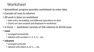
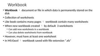
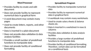
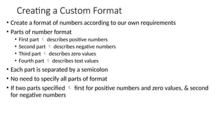
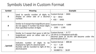
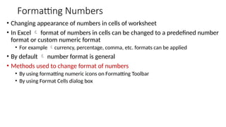
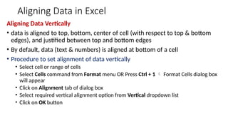
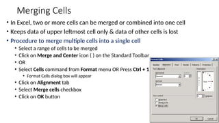
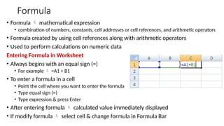
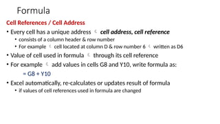
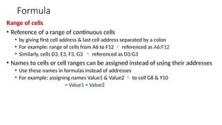
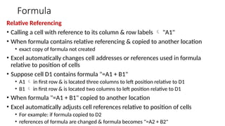
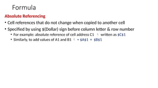
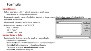
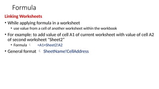
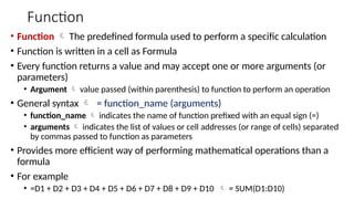
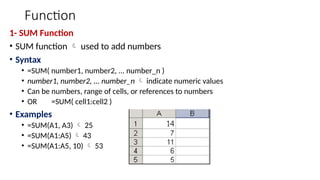
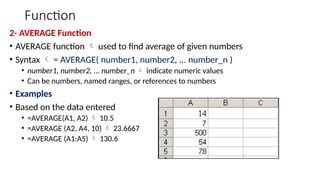
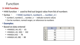
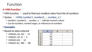
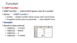
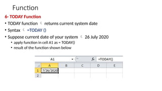
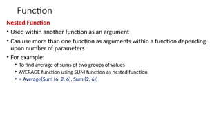
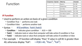
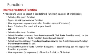
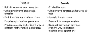
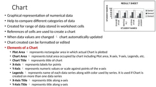
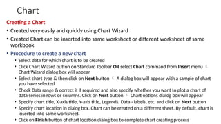
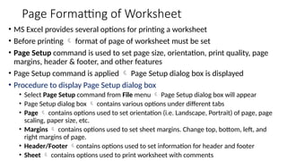
2. Chapter 9
Spreadsheet Software
COMPUTER SCIENCE – 11

3. Contents
• Spreadsheet Program
• Worksheet & Workbook
• Microsoft Excel
• Entering Data into Worksheet
• Cell Formatting
• Formatting Numbers
• Aligning Data in Excel
• Merging Cells
• Formula
• Function
• Chart
• Page Formatting of Worksheet
• Printing in Worksheet

4. Spreadsheet Program
Q.1 What is spreadsheet program? Explain the basic features of spreadsheet
program.

5. Spreadsheet Program
• Computer program used to store & process data in rows and columns in an
electronic spreadsheet
• Application program
• Provides a large number of electronic spreadsheets to enter & process data
• Sheets  worksheets
• Can perform calculations on numerical data
• Also provides methods for analyzing all types of data & presenting data in
graphical form etc.
• Spreadsheet program  Microsoft Excel

6. Features of Spreadsheet Program
1. Grid of Rows and Columns
• Spreadsheet  grid of rows & columns
• Columns  labeled with letters A, B, C,…. etc.
• Rows  labeled with numbers 1, 2, 3, 4,… etc.
• Cell  Intersection of a row and a column
• Reference Number  Address of cell formed by combining column number & row number
• such as "A1", "B18" etc.
• Label or value  data stored in a cell
• "label“  text entry such as "Total Marks“
• "value“  can be a number, a date, a formula or a formula’s result
2. Formulas
• Used to perform calculations on numeric data
• When formula used  calculated result is displayed in cell
3. Built-in Functions
• Spreadsheet program contains a large number of built-in functions
• Used to perform different tasks (or calculations i.e. arithmetic or statistical calculations)

7. Features of Spreadsheet Program
4. Commands
• Used to manipulate worksheet or its contents
• These commands are grouped in Menu bar
5. Text Manipulation
• Provides features to perform various operations for manipulations of text
data
6. Creating charts in Excel
• User can create charts for numerical data
• Easy to compare & to understand numerical data
7. Printing
• Allows user to make a hardcopy of data stored in worksheet

8. Worksheet & Workbook
Q.2 What do you know about Worksheet and Workbook?

9. Worksheet
• Spreadsheet program provides worksheets to enter data
• Consists of rows & columns
• All work is done on worksheet
• data entry, formatting, and different operations on data
• Charts are also created and displayed in worksheet
• In Excel  worksheet consists of 256 columns & 65536 rows
• rows
• arranged horizontally
• labeled with numbers 1, 2, 3, 4,… etc.
• columns
• arranged vertically
• labeled with letters A, B, C,…. etc.

10. Workbook
• Workbook  document or file in which data is permanently stored on the
disk
• Collection of worksheets
• Like book contains many pages  workbook contain many worksheets
• When new workbook created  by default 3 worksheets
• Can add new worksheets in a workbook
• Can also delete worksheets from workbook
• However, must have at least one worksheet
• In MS-Excel  workbook saved with file extension ".xls"

11. Word Processor
• Provides facility to create and edit
document
• Does not provide facility to represent
numerical data in graphical form
• A word document may contain many
pages
• Used to create letters, reports, and other
documents
• Data is inserted in a plain document
• Does not provide data validation & data
analysis facilities
• Provides a small number of predefined
functions to manipulate data
• Does not provide facility of conditional
formatting
Spreadsheet Program
• Provides facility to manipulate numerical
data
• Provides facility to represent numerical
data in graphical form
• A workbook may contain many worksheets
• Used to create salary sheets & balance
sheets etc.
• Data is inserted in a worksheet in rows &
columns
• Provides data validation & data analysis
facilities
• Provides a large number of predefined
functions to manipulate data
• Provides facility of conditional formatting.
Therefore, certain data can be formatted
on a conditional basis

12. Microsoft Excel
Q.4 What is Microsoft Excel? Write the procedure to start Excel.
Q.5 Describe the Spreadsheet’s Interface and its elements.

13. Microsoft Excel
• Procedure to start Microsoft Excel
• Click Start button  Start menu will appear
• Choose Programs from Start menu  submenu of Programs will appear
• Select Microsoft Excel from Program menu
• When Microsoft Excel successfully loaded into memory  interface window will appear

14. Spreadsheet’s Interface
1. Title Bar
• Located at top of Interface window
• Displays Microsoft Excel + name of opened workbook on Title bar
• For example  for new workbook  "Microsoft Excel - Book1"
• When workbook saved by giving a proper name  name appears in Title bar
2. Menu Bar
• Commands used to perform different tasks during creating or editing workbooks are grouped
together into Menu Bar
3. Toolbars
• Shortcuts to commands  commands in menus
• Standard Toolbar
• Contains shortcut command buttons for performing commonly used tasks
• Tasks  opening & saving documents, copying, and moving information, etc.
• Formatting Toolbar
• Contains formatting command buttons & options
• Buttons or options  used to apply commonly used text formats

15. Spreadsheet’s Interface
4. Cell
• Cell  Intersection of a column and a row
• Data is entered into cells of worksheet
5. Active Cell
• The currently selected cell where data can be entered or edited
• When another cell is selected or cursor is moved to another cell  that cell
becomes Active Cell
6. Cell Address
• Unique address of each cell  represents position or location of a specific cell
• Cell address  location of a cell in a worksheet, cell reference
• Consists of a column letter & row number that intersect at location of cell
• For example  cell located in column 3 & row 6  represented as C6
• Used in formulas, functions, charts & other Excel commands

16. Spreadsheet’s Interface
7. Column Header
• A horizontal bar that has headings of columns with labels A, B, C, and so on
• Usually used to select columns of worksheet
8. Row Header
• A vertical bar that has headings of rows with labels 1, 2, 3, and so on
• Usually used to select rows of worksheet
9. Formula Bar
• When formula is used in a cell  calculated result displayed
• Actual formula displayed  in Formula Bar
• If formula not applied  contents of cell displayed in Formula bar
• Also used to edit contents of cell
10. Status Bar
• At the bottom of Microsoft Excel window
• Shows basic information about opened workbook

17. Spreadsheet’s Interface
11. Sheet Tabs
• Each worksheet has tab at bottom of Excel window
• User can easily switch between worksheets by clicking one of these tabs
• Unique name
• When new workbook created  consists of 3 worksheets
• Names  Sheet1, Sheet2, & Sheet3
• Names can be changed
12. Horizontal Scroll Bar
• At the bottom border of Excel window
• Used to scroll worksheet left & right  to see contents of cells
13. Vertical Scroll Bar
• At the right border of Excel window
• Used to scroll worksheet up & down  to see contents of cells

18. Entering Data into Worksheet
Q.6 How is data entered into the worksheet?

19. Entering Data into Worksheet
• Cell  basic unit where data is entered
• Data  alphabetical characters (or text), numbers, dates, and formulas
• Enter key is pressed to complete data entry
• When Enter key pressed  cursor automatically moves one row down
• Cell can also hold graphics etc.
• When formula entered  not shown in cell but its result is shown
• States of a cell
• Active Cell  currently selected cell where data can be entered or edited
• A bold rectangular border indicates an active cell
• When another cell selected or cell pointer is moved to another cell  that cell becomes
Active Cell
• At a time  single cell is active
• While other cells are inactive
• Inactive cells  passive cells

20. Cell Formatting
Q.7 What is cell formatting and how is the custom format created?

21. Cell Formatting
• Process of changing appearance of text
• General format  Default format assigned to a cell
• displays data as it is entered
• If cell not wide enough to display a long decimal number 
• General format rounds off number
• Uses scientific notation for large or small numbers
• For example: 0.0000000001  displayed as 1E-10
• Change appearance of data
• by changing font, font style, and font size
• by aligning data in cells
• by setting a numeric format
• by setting style & color of cell border etc.
• Ways to format cells
• By using Formatting toolbar
• By using Format Cells dialog box

22. Creating a Custom Format
• Create a format of numbers according to our own requirements
• Parts of number format
• First part  describes positive numbers
• Second part  describes negative numbers
• Third part  describes zero values
• Fourth part  describes text values
• Each part is separated by a semicolon
• No need to specify all parts of format
• If two parts specified  first for positive numbers and zero values, & second
for negative numbers

23. Symbols Used in Custom Format
Symbol Meaning Example
0
Used to specify number of digits to
display on either side of a decimal
number.
Custom format  0000
• 12  0012
• 450  0450
#
Similar to 0 except that insignificant zeros
do not appear if number has fewer digits
than specified number of digits
Custom format  #,###
• 1500  1,500
?
Similar to 0 except that space is left for
insignificant zeros on either side of a
decimal point
Custom format  0.???
16.545 & 2.4 displayed vertically
Decimal point of 16.545 will become under the
decimal point of 2.4
. (period)
Indicates number of digits to be
displayed to right of a decimal point
Number will be rounded to right of the
decimal point
Custom format  ###.00
• 1.2  1.20
• 58  58.00
• 58.888715  58.89

24. Formatting Numbers
Q.9 What is meant by formatting numbers? Explain the procedure to format
numbers using Formatting Numeric icons and Format dialog box.

25. Formatting Numbers
• Changing appearance of numbers in cells of worksheet
• In Excel  format of numbers in cells can be changed to a predefined number
format or custom numeric format
• For example currency, percentage, comma, etc. formats can be applied
• By default  number format is general
• Methods used to change format of numbers
• By using formatting numeric icons on Formatting Toolbar
• By using Format Cells dialog box

26. Formatting Numbers
Formatting using Numeric Icons
• Easiest & simplest way to change formatting of numbers in cells
• Select cell or range of cells that contain numeric data & click one of “Formatting Numeric Icons” on
Formatting Toolbar
• Currency
• Used to apply currency format to numeric data
• Numbers in cells displayed prefixed with currency symbol  $200
• Also change currency symbol (e.g. Rs.) from Control Panel of Windows
• Percent
• Used to apply percentage format to numbers
• For example: 0.55  55%
• Comma
• Used to apply a comma format
• For example: 63540  63,540.00
• Increase Decimal
• Used to increase number of decimal places in numeric data of selected cells
• Decrease Decimal
• Used to decrease number of decimal places in numeric data of selected cells

27. Formatting Numbers
Formatting Numbers using Format Cells Dialog Box
• Provides many styles of number formatting
• Styles  scientific, accounting, date, time, etc.
• Number format can be customized
• Procedure to apply formatting to numeric data of selected cells
• Select cell or range of cells
• Select Cells command from Format menu OR Press Ctrl + 1  Format Cells dialog box
will appear
• Click on Number tab of dialog box
• Select number format from Category list box and select other options from dialog box
(if required)
• Click on OK button to apply settings

28. Aligning Data in Excel
Q.10 What is meant by aligning data in Excel? Explain the procedure to align the
data horizontally and vertically.

29. Aligning Data in Excel
• Data stored into cells can be aligned to left, right, center, top or bottom of the cell
Aligning Data Horizontally
• In horizontal alignment, data is aligned to the left of the cell, right of the cell, center of the cell, and
justified (with respect to the left and right edges of the cell). By default, texts are aligned to left and
numbers are aligned to the right of the cell.
• Procedure to set alignment of data horizontally
• Select cell or range of cells
• Click one of alignment buttons on Formatting Toolbar
• Left Alignment Button
• Left alignment aligned to left edge of cell
• Right Alignment Button
• Right alignment  aligned to right edge of cell
• Center Alignment Button
• Center alignment  aligned to center or middle of cell
• OR
• Select Cells command from Format menu OR Press Ctrl + 1  Format Cells dialog box will appear
• Click on Alignment tab of dialog box
• Select required horizontal alignment option from Horizontal dropdown list
• Click on OK button

30. Aligning Data in Excel
Aligning Data Vertically
• data is aligned to top, bottom, center of cell (with respect to top & bottom
edges), and justified between top and bottom edges
• By default, data (text & numbers) is aligned at bottom of a cell
• Procedure to set alignment of data vertically
• Select cell or range of cells
• Select Cells command from Format menu OR Press Ctrl + 1  Format Cells dialog box
will appear
• Click on Alignment tab of dialog box
• Select required vertical alignment option from Vertical dropdown list
• Click on OK button

31. Merging Cells
Q.11 Describe the procedure to merge cells in a worksheet.

32. Merging Cells
• In Excel, two or more cells can be merged or combined into one cell
• Keeps data of upper leftmost cell only & data of other cells is lost
• Procedure to merge multiple cells into a single cell
• Select a range of cells to be merged
• Click on Merge and Center icon ( ) on the Standard Toolbar
• OR
• Select Cells command from Format menu OR Press Ctrl + 1
• Format Cells dialog box will appear
• Click on Alignment tab
• Select Merge cells checkbox
• Click on OK button

33. Formula
Q.12 What is a formula and how the formula is entered into Excel?
Q.13 What is cell reference /cell address and range of cells?
Q.14 Differentiate between Relative Referencing and Absolute Referencing.
Q.15 What do you understand by the term named ranges? How is the range of cells named?
Q.16 How are the cells of different Worksheets linked?

34. Formula
• Formula  mathematical expression
• combination of numbers, constants, cell addresses or cell references, and arithmetic operators
• Formula created by using cell references along with arithmetic operators
• Used to perform calculations on numeric data
Entering Formula in Worksheet
• Always begins with an equal sign (=)
• For example  =A1 + B1
• To enter a formula in a cell
• Point the cell where you want to enter the formula
• Type equal sign (=)
• Type expression & press Enter
• After entering formula  calculated value immediately displayed
• If modify formula  select cell & change formula in Formula Bar

35. Formula
Cell References / Cell Address
• Every cell has a unique address  cell address, cell reference
• consists of a column header & row number
• For example  cell located at column D & row number 6  written as D6
• Value of cell used in formula  through its cell reference
• For example  add values in cells G8 and Y10, write formula as:
= G8 + Y10
• Excel automatically, re-calculates or updates result of formula
• if values of cell references used in formula are changed

36. Formula
Range of cells
• Reference of a range of continuous cells
• by giving first cell address & last cell address separated by a colon
• For example: range of cells from A6 to F12  referenced as A6:F12
• Similarly, cells D3, E3, F3, G3  referenced as D3:G3
• Names to cells or cell ranges can be assigned instead of using their addresses
• Use these names in formulas instead of addresses
• For example: assigning names Value1 & Value2  to cell G8 & Y10
= Value1 + Value2

37. Formula
Relative Referencing
• Calling a cell with reference to its column & row labels  "A1"
• When formula contains relative referencing & copied to another location
• exact copy of formula not created
• Excel automatically changes cell addresses or references used in formula
relative to position of cells
• Suppose cell D1 contains formula "=A1 + B1"
• A1  in first row & is located three columns to left position relative to D1
• B1  in first row & is located two columns to left position relative to D1
• When formula "=A1 + B1" copied to another location
• Excel automatically adjusts cell references relative to position of cells
• For example: if formula copied to D2
• references of formula are changed & formula becomes "=A2 + B2"

38. Formula
Absolute Referencing
• Cell references that do not change when copied to another cell
• Specified by using $(Dollar) sign before column letter & row number
• For example: absolute reference of cell address C1  written as $C$1
• Similarly, to add values of A1 and B1  = $A$1 + $B$1

39. Formula
Named Ranges
• Select a range of cells  give it a name as a reference
• Give a name to a single cell as a reference
• Easy way to specify range of cells in a formula or to go to specified cell or range of cells with the
reference to its name
• Also make it easier to understand formulas
• For example: formula =C10*100/C8
• C10  "Marks"
• C8  "Total“
• =Marks * 100 / Total
Naming Range of Cells
• Procedure to define a name for a cell or range of cells
• Select cell or range of cells
• From Insert menu select Name command  submenu will appear
• Select Define from submenu  dialog box will appear
• Type name of range in Names in workbook textbox
• Click on OK button of the dialog box.

40. Formula
Linking Worksheets
• While applying formula in a worksheet
• use value from a cell of another worksheet within the workbook
• For example: to add value of cell A1 of current worksheet with value of cell A2
of second worksheet "Sheet2“
• Formula  =A1+Sheet2!A2
• General format  SheetName!CellAddress

41. Function
Q.17 What is a function? Briefly describe the commonly used functions in MS
Excel.

42. Function
• Function  The predefined formula used to perform a specific calculation
• Function is written in a cell as Formula
• Every function returns a value and may accept one or more arguments (or
parameters)
• Argument  value passed (within parenthesis) to function to perform an operation
• General syntax  = function_name (arguments)
• function_name  indicates the name of function prefixed with an equal sign (=)
• arguments  indicates the list of values or cell addresses (or range of cells) separated
by commas passed to function as parameters
• Provides more efficient way of performing mathematical operations than a
formula
• For example
• =D1 + D2 + D3 + D4 + D5 + D6 + D7 + D8 + D9 + D10  = SUM(D1:D10)

43. Function
1- SUM Function
• SUM function  used to add numbers
• Syntax
• =SUM( number1, number2, ... number_n )
• number1, number2, ... number_n  indicate numeric values
• Can be numbers, range of cells, or references to numbers
• OR =SUM( cell1:cell2 )
• Examples
• =SUM(A1, A3)  25
• =SUM(A1:A5)  43
• =SUM(A1:A5, 10)  53

44. Function
2- AVERAGE Function
• AVERAGE function  used to find average of given numbers
• Syntax  = AVERAGE( number1, number2, ... number_n )
• number1, number2, ... number_n  indicate numeric values
• Can be numbers, named ranges, or references to numbers
• Examples
• Based on the data entered
• =AVERAGE(A1, A2)  10.5
• =AVERAGE (A2, A4, 10)  23.6667
• =AVERAGE (A1:A5)  130.6

45. Function
3- MAX Function
• MAX function  used to find out largest value from list of numbers
• Syntax  = MAX( number1, number2, ... number_n )
• number1, number2, ... number_n  indicate numeric values
• Can be numbers, named ranges, or references to numbers
• Examples:
• Based on data entered
• =MAX(A2, A4, A5)  65
• =MAX(A1, A5, 102)  102
• =MAX(A1:A5)  78
• =MAX(A1:A5, 88)  88

46. Function
4- MIN Function
• MIN function  used to find out smallest value from list of numbers
• Syntax  =MIN( number1, number2, ... number_n )
• number1, number2, ... number_n  indicate numeric values
• Can be numbers, named ranges, or references to numbers
• Examples
• Based on data entered
• =MIN(A2, A4, A5)  14
• =MIN(A1, A5, 2)  2
• =MIN(A1:A5)  12
• =MIN(A1:A5, -88)  -88

47. Function
5- SQRT Function
• SQRT function  used to find square root of a number
• Syntax  =SQRT( number )
• number  positive number whose square root is to be found
• If negative number given as parameter  return #NUM! error
• Examples
• Based on data entered
• =SQRT(A1)  3.741657
• =SQRT(A2)  #NUM!
• =SQRT(A3)  3
• =SQRT(A4)  9.176056

48. Function
6- TODAY Function
• TODAY function  returns current system date
• Syntax  =TODAY ()
• Suppose current date of your system  26 July 2020
• apply function in cell A1 as = TODAY()
• result of the function shown below

49. Function
Nested Function
• Used within another function as an argument
• Can use more than one function as arguments within a function depending
upon number of parameters
• For example:
• To find average of sums of two groups of values
• AVERAGE function using SUM function as nested function
• = Average(Sum (6, 2, 6), Sum (2, 6))

50. Function
IF Function
• Used to perform an action on basis of a given condition
• Condition True  performs one task
• Condition False  performs another task
• Syntax  IF(Condition, Task1,Task2)
• Condition  indicates given condition  A10 >= 100
• Task1  indicates task or value that computer will take action if condition is True
• Task2  indicates task or value that computer will take action if condition is False
• For example  IF function will display "Pass" if value in cell B1 is greater than
40; otherwise display "Fail": = IF(B1>40, "Pass", "Fail")

51. Function
Inserting Predefined Function
• Procedure used to insert a predefined function in a cell of worksheet
• Select cell to insert function
• Type = sign & type name of function
• Give arguments in parenthesis after function names (if required)
• Press Enter key. The result will appear in cell
• OR
• Select cell to insert function
• Select Function command from Insert menu OR Click Paste Function icon ( ) on the
Standard Toolbar  Paste Function dialog box will appear
• Select function category from Function Category list box & select required function
from Function name list box
• Click on Ok button of Paste Function dialog box  second dialog box will appear for
function arguments
• Give arguments (or arguments) of function & click on Ok button

52. Function
• Built-in in spreadsheet program
• Can only perform predefined
function
• Each function has a unique name
• Require arguments or parameters.
• Provides an easy and efficient way to
perform mathematical operations
Formula
• Created by user
• Can perform function as required by
user
• Formula has no name
• Does not require parameters
• Does not provide an easy and
efficient way to perform
mathematical operations

53. Chart
Q.20 What is a Chart? Describe the elements of a chart.

54. Chart
• Graphical representation of numerical data
• Help to compare different categories of data
• Created for range of data stored in worksheet cells
• References of cells are used to create a chart
• When data values are changed  chart automatically updated
• Chart created can be formatted or edited
• Elements of a Chart
• Plot Area  represents rectangular area in which actual Chart is plotted
• Chart Area  represents total area occupied by chart including Plot area, X-axis, Y-axis, Legends, etc.
• Chart Title  represents title of chart
• X-Axis  represents labels for points
• Y-Axis  represents numeric values or scale against points of the x-axis
• Legends  represents name of each data series along with color used by series. It is used if Chart is
created on more than one data series
• X-Axis Title  represents title along x-axis
• Y-Axis Title  represents title along y-axis

55. Chart
Creating a Chart
• Created very easily and quickly using Chart Wizard
• Created Chart can be inserted into same worksheet or different worksheet of same
workbook
• Procedure to create a new chart
• Select data for which chart is to be created
• Click Chart Wizard button on Standard Toolbar OR select Chart command from Insert menu 
Chart Wizard dialog box will appear
• Select chart type & then click on Next button  A dialog box will appear with a sample of chart
you have selected
• Check Data range & correct it if required and also specify whether you want to plot a chart of
data series in rows or columns. Click on Next button  Chart options dialog box will appear
• Specify chart title, X-axis title, Y-axis title, Legends, Data - labels, etc. and click on Next button
• Specify chart location in dialog box. Chart can be created on a different sheet. By default, chart is
inserted into same worksheet.
• Click on Finish button of chart location dialog box to complete chart creating process

56. Page Formatting of Worksheet
Q.22 How is the page of the worksheet formatted? Explain the purpose of various
tabs of the Page Setup dialog box

57. Page Formatting of Worksheet
• MS Excel provides several options for printing a worksheet
• Before printing  format of page of worksheet must be set
• Page Setup command is used to set page size, orientation, print quality, page
margins, header & footer, and other features
• Page Setup command is applied  Page Setup dialog box is displayed
• Procedure to display Page Setup dialog box
• Select Page Setup command from File menu  Page Setup dialog box will appear
• Page Setup dialog box  contains various options under different tabs
• Page  contains options used to set orientation (i.e. Landscape, Portrait) of page, page
scaling, paper size, etc.
• Margins  contains options used to set sheet margins. Change top, bottom, left, and
right margins of page.
• Header/Footer contains options used to set information for header and footer
• Sheet  contains options used to print worksheet with comments

58. Printing in Worksheet
Q.23 How is a worksheet printed on the printer? Briefly describe the main
printing options in MS Excel.

59. Printing in Worksheet
• Printing a worksheet is different than printing a Word document
• because worksheet can be so wide & tall
• In MS Excel, worksheet is printed after adjusting page setup
• If worksheet is printed without adjusting page setup  MS Excel uses default page
setting
• page size, page margins, printing direction before printing worksheet can be
changed
• Print a selected area of worksheet or an entire worksheet
• Similarly, Take one or multiple copies of worksheet
• Procedure to print a worksheet on the printer
• Select Print from File menu  Print dialog box will appear
• Select your options from Print dialog box
• Click on OK button to send data on printer

60. Printing in Worksheet
Printing Options
• Printer
• Used to select printer
• To select name of printer installed in computer  click on Name dropdown list box and
select printer
• Print range
• Used to select range of pages to be printed
• Select a range of pages or the entire worksheet
• Copies
• Number of copies of selected page or range of pages is specified
• Printing a complete worksheet is very easy
• Just click Print icon on toolbar to print active sheet
• Print Preview command should be used before sending to print
• Note  chart can be printed in a similar way as a worksheet

61. For more details, refers to
PM Series
Computer Science
ICS Part-1
by
CM Aslam, Aqsa Aslam, Mudassir Ahmad & Atif
Mansoor
Publisher: Majeed Sons
22- Urdu Bazar, Lahore