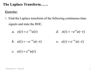
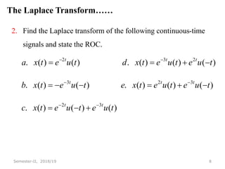
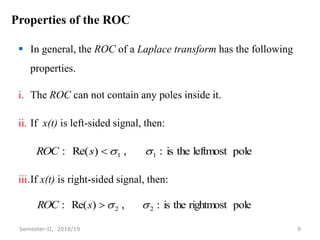
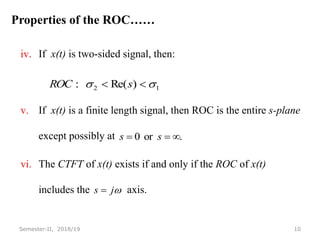
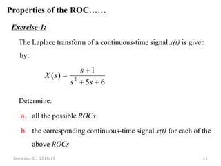
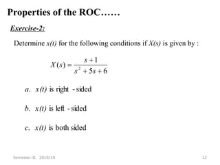
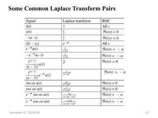
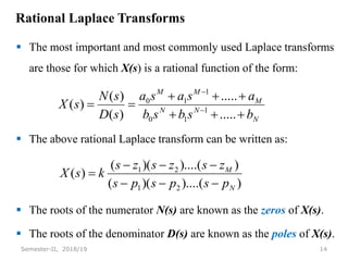
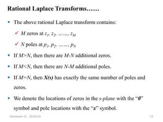
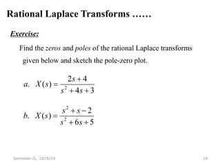
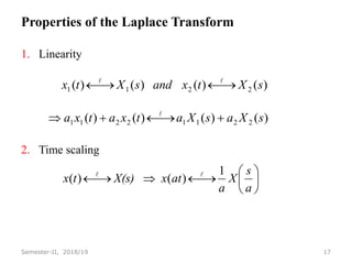
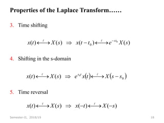
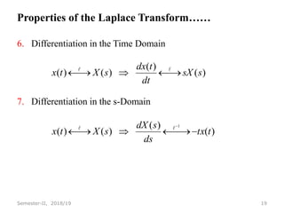
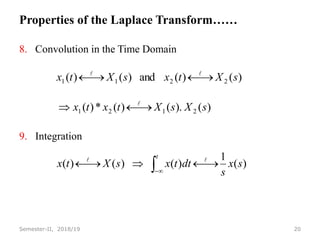
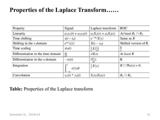
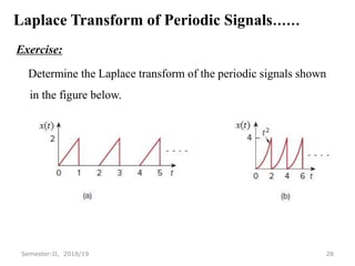
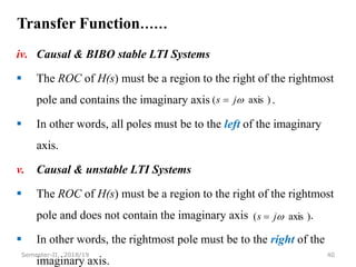
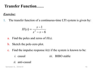
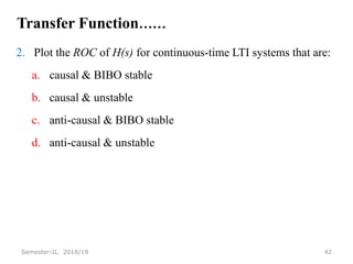
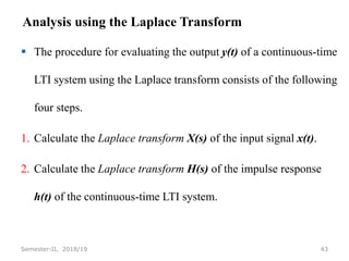
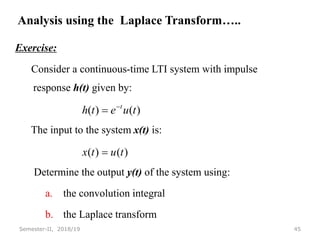
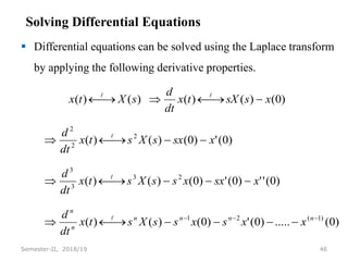
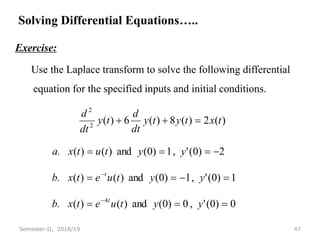
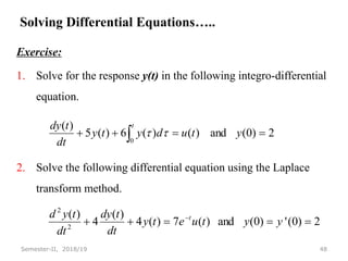
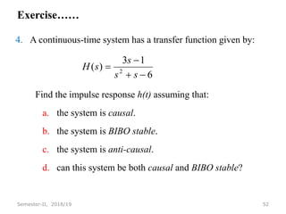
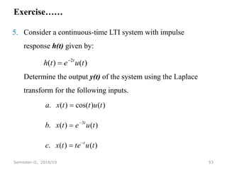
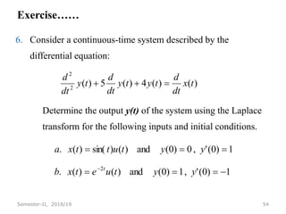
This document provides an overview of the Laplace transform and its inverse. It defines the Laplace transform, discusses properties such as linearity and time shifting. It also covers the region of convergence, rational Laplace transforms containing poles and zeros, and properties related to differentiation and integration in both the time and s-domains. Examples are provided to find Laplace transforms and illustrate properties. Periodic signals are also discussed, showing how they can be represented as the sum of shifted components, and taking the Laplace transform using time shifting properties.

1. Chapter Four
Laplace Transform and Its Inverse
Addis Ababa Science and Technology University
College of Electrical & Mechanical Engineering
Electrical & Computer Engineering Department
Signals and Systems Analysis (EEEg-2121)

2. Laplace Transform and Its Inverse
Outline
 Introduction
 The Laplace Transform
 Properties of the ROC
 Properties of the Laplace Transform
 Inverse Laplace Transform
 Transfer Function
 Analysis using the Laplace Transform
 Solving Differential Equations
Semester-II, 2018/19 2

3. Introduction
 The Laplace transform is a generalization of the Fourier
transform of a continuous time signal.
 The Laplace transform converges for signals for which the
Fourier transform does not.
 Hence, the Laplace transform is a useful tool in the analysis and
design of continuous time systems.
3
Semester-II, 2018/19

4. The Laplace Transform
 The Laplace transform of a continuous-time signal x(t), denoted
by X(s), is defined as:
 The complex variable s is of the form with a real
part and an imaginary part .
 The Laplace transform defined by the above equation is known
as the bilateral Laplace transform.
4
Semester-II, 2018/19





 dt
e
t
x
s
X st
)
(
)
(

 j
s 

 

5. The Laplace Transform……
 We say that x(t) and X(s) are Laplace transform pairs and denote
this relationship as:
 The unilateral Laplace transform plays an important role in
the analysis of causal systems described by constant coefficient
linear differential equations with initial conditions.
 The unilateral Laplace transform is mathematically defined as:
5
Semester-II, 2018/19
)
certain
(with
)
(
)
( ROC
s
X
t
x 





0
)
(
)
( dt
e
t
x
s
X st

6. The Laplace Transform……
Region of Convergence (ROC):
 The region of convergence (ROC) is defined as the set of all
values of s for which X(s) has a finite values.
 Every time we calculate the Laplace transform, we should
indicate its ROC.
6
Semester-II, 2018/19

7. The Laplace Transform……
Exercise:
1. Find the Laplace transform of the following continuous-time
signals and state the ROC.
7
Semester-II, 2018/19
)
(
)
(
.
)
(
)
(
.
)
(
)
(
.
)
(
)
(
.
)
(
)
(
.
t
u
e
t
x
c
t
u
e
t
x
e
t
u
e
t
x
b
t
u
e
t
x
d
t
u
e
t
x
a
at
at
at
at
at














8. The Laplace Transform……
2. Find the Laplace transform of the following continuous-time
signals and state the ROC.
8
Semester-II, 2018/19
)
(
)
(
)
(
.
)
(
)
(
)
(
.
)
(
)
(
.
)
(
)
(
)
(
.
)
(
)
(
.
3
2
3
2
3
2
3
2
t
u
e
t
u
e
t
x
c
t
u
e
t
u
e
t
x
e
t
u
e
t
x
b
t
u
e
t
u
e
t
x
d
t
u
e
t
x
a
t
t
t
t
t
t
t
t




















9. Properties of the ROC
 In general, the ROC of a Laplace transform has the following
properties.
i. The ROC can not contain any poles inside it.
ii. If x(t) is left-sided signal, then:
iii.If x(t) is right-sided signal, then:
9
Semester-II, 2018/19
pole
rightmost
the
is
:
,
)
Re(
: 2
2 


s
ROC
pole
leftmost
the
is
:
,
)
Re(
: 1
1 


s
ROC

10. Properties of the ROC……
iv. If x(t) is two-sided signal, then:
v. If x(t) is a finite length signal, then ROC is the entire s-plane
except possibly at
vi. The CTFT of x(t) exists if and only if the ROC of x(t)
includes the axis.
10
Semester-II, 2018/19
)
Re(
: 1
2 
 
 s
ROC
.
or
0 

 s
s

j
s 

11. Properties of the ROC……
Exercise-1:
The Laplace transform of a continuous-time signal x(t) is given
by:
Determine:
a. all the possible ROCs
b. the corresponding continuous-time signal x(t) for each of the
above ROCs
11
Semester-II, 2018/19
6
5
1
)
( 2




s
s
s
s
X

12. Properties of the ROC……
Exercise-2:
Determine x(t) for the following conditions if X(s) is given by :
12
Semester-II, 2018/19
6
5
1
)
( 2




s
s
s
s
X
sided
both
is
.
sided
-
left
is
.
sided
-
right
is
.
x(t)
c
x(t)
b
x(t)
a

13. Some Common Laplace Transform Pairs
13
Semester-II, 2018/19

14. Rational Laplace Transforms
 The most important and most commonly used Laplace transforms
are those for which X(s) is a rational function of the form:
 The above rational Laplace transform can be written as:
 The roots of the numerator N(s) are known as the zeros of X(s).
 The roots of the denominator D(s) are known as the poles of X(s).
14
Semester-II, 2018/19
N
N
N
M
M
M
b
s
b
s
b
a
s
a
s
a
s
D
s
N
s
X







 

.....
.....
)
(
)
(
)
( 1
1
0
1
1
0
)
)....(
)(
(
)
)....(
)(
(
)
(
2
1
2
1
N
M
p
s
p
s
p
s
z
s
z
s
z
s
k
s
X








15. Rational Laplace Transforms……
 The above rational Laplace transform contains:
 M zeros at z1, z2, ……, zM
 N poles at p1, p2, ……, pN
 If M>N, then there are M-N additional zeros.
 If M<N, then there are N-M additional poles.
 If M=N, then X(s) has exactly the same number of poles and
zeros.
 We denote the locations of zeros in the s-plane with the “0”
symbol and pole locations with the “x” symbol.
15
Semester-II, 2018/19

16. Rational Laplace Transforms ……
Exercise:
Find the zeros and poles of the rational Laplace transforms
given below and sketch the pole-zero plot.
16
Semester-II, 2018/19
5
6
2
)
(
.
3
4
4
2
)
(
.
2
2
2









s
s
s
s
s
X
b
s
s
s
s
X
a

17. Properties of the Laplace Transform
1. Linearity
2. Time scaling
17
Semester-II, 2018/19
)
(
)
(
)
(
)
(
)
(
)
(
)
(
)
(
2
2
1
1
2
2
1
1
2
2
1
1
s
X
a
s
X
a
t
x
a
t
x
a
s
X
t
x
and
s
X
t
x























a
s
X
a
at
x
X(s)
t
x
1
)
(
)
( 


18. Properties of the Laplace Transform……
3. Time shifting
4. Shifting in the s-domain
5. Time reversal
18
Semester-II, 2018/19
)
(
)
(
)
(
)
( 0
0 s
X
e
t
t
x
s
X
t
x st






 

)
(
)
(
)
(
)
( s
X
t
x
s
X
t
x 





 

   
0
0
)
(
)
( s
s
X
t
x
e
s
X
t
x t
s





 


19. Properties of the Laplace Transform……
6. Differentiation in the Time Domain
7. Differentiation in the s-Domain
19
Semester-II, 2018/19
)
(
)
(
)
(
)
( s
sX
dt
t
dx
s
X
t
x 



 

)
(
)
(
)
(
)
(
1
t
tx
ds
s
dX
s
X
t
x 









20. Properties of the Laplace Transform……
8. Convolution in the Time Domain
9. Integration
20
Semester-II, 2018/19
)
(
1
)
(
)
(
)
( s
x
s
dt
t
x
s
X
t
x
t




 



)
(
).
(
)
(
*
)
(
)
(
)
(
and
)
(
)
(
2
1
2
1
2
2
1
1
s
X
s
X
t
x
t
x
s
X
t
x
s
X
t
x











21. Properties of the Laplace Transform……
21
Semester-II, 2018/19
Table: Properties of the Laplace transform

22. Properties of the Laplace Transform……
Exercise:
Find the Laplace transform and state the ROC of the following
continuous-time signals using properties of the Laplace
transform.
22
Semester-II, 2018/19
)
(
3
cos
)
(
.
)
(
)
(
.
)
(
2
sin
)
(
.
)
4
(
2
)
(
.
)
(
3
)
(
2
)
(
)
(
.
2
3
2
2
t
tu
te
t
x
c
t
u
e
t
t
x
e
t
tu
t
t
x
b
t
tu
t
x
d
t
u
e
t
u
t
t
x
a
t
t
t










 

23. Properties of the Laplace Transform……
Exercise:
Find the Laplace transform of the following continuous-time
signals using properties of the Laplace transform.
23
Semester-II, 2018/19

24. Laplace Transform of Periodic Signals
 Consider the continuous-time periodic signal x(t) shown in the
figure given below.
 The above periodic signal can be represented as the sum of
time-shifted signal components as:
24
Semester-II, 2018/19
(i)
T
t
x
T
t
x
t
x
t
x
t
x
t
x
t
x
.........
)
2
(
)
(
)
(
.........
)
(
)
(
)
(
)
(
1
1
1
3
2
1











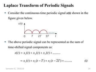
25. Laplace Transform of Periodic Signals……
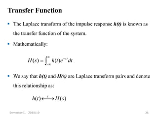
 Note that the signal x1(t) can be expressed as:
25
Semester-II, 2018/19
Fig. Decomposition of the periodic signal into its components




 





otherwise
,
0
0
,
)
(
)]
(
)
(
)[
(
)
(
1
T
t
t
x
T
t
u
t
u
t
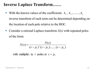
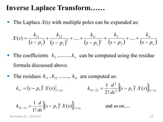
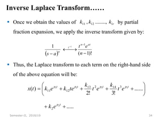
x
t
x

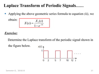
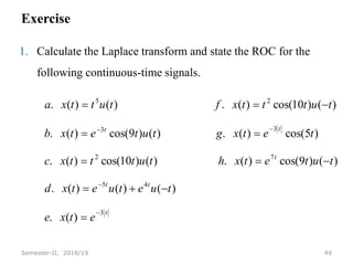
26. Laplace Transform of Periodic Signals……
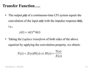
 Taking the Laplace transform of both sides of equation (i) by
applying time-shifting property, we get:
 Consider the geometric series formula given by:
26
Semester-II, 2018/19
(ii)
e
e
e
s
X
e
s
X
e
s
X
e
s
X
s
X
s
X
Ts
Ts
Ts
Ts
Ts
Ts
......]
1
)[
(
....
)
(
)
(
)
(
)
(
)
(
3
2
1
3
1
2
1
1
1
















1
,
1
1
......
1 3
2
0











r
r
r
r
r
r
k
k

27. Laplace Transform of Periodic Signals……
 Applying the above geometric series formula to equation (ii), we
obtain:
Exercise:
Determine the Laplace transform of the periodic signal shown in
the figure below.
27
Semester-II, 2018/19
1
)
(
)
( 1
Ts
e
s
X
s
X 



28. Laplace Transform of Periodic Signals……
Exercise:
Determine the Laplace transform of the periodic signals shown
in the figure below.
28
Semester-II, 2018/19

29. Inverse Laplace Transform
Inverting by Inspection:
 The simplest inversion method is by inspection, or by comparing
with the table of common Laplace transform pairs.
Exercise:
Find the inverse of the following Laplace transforms by
inspection.
29
Semester-II, 2018/19
2
)
Re(
:
,
2
1
)
(
.
2
)
Re(
:
,
2
1
)
(
.








s
ROC
s
s
X
b
s
ROC
s
s
X
a

30. Inverse Laplace Transform……
Inverting by Partial Fractional Expansion:
 This is a method of writing complex rational Laplace transforms
as a sum of simple terms.
 After expressing the complex rational Laplace transform as a sum
of simple terms, each term can be inverted by inspection.
 Consider a rational Laplace transform X(s) of the form:
with the order of N(s) less than the order of the denominator
polynomial D(s).
30
Semester-II, 2018/19
)
(
)
(
)
(
s
D
s
N
s
X 

31. Inverse Laplace Transform……
 If poles are distinct, the rational Laplace
transform X(s) can be expanded using partial fraction expansion
as:
 The coefficients are called the residues of the
partial fraction expansion. The residues are computed as:
31
Semester-II, 2018/19
     
n
n
p
s
k
p
s
k
p
s
k
s
X






 .......
)
(
2
2
1
1
n
p
p
p ........,
,
, 2
1
n
k
k
k ........,
,
, 2
1
  i
p
s
i
i s
X
p
s
k 

 )
(

32. Inverse Laplace Transform……
 With the known values of the coefficients
inverse transform of each term can be determined depending on
the location of each pole relative to the ROC.
 Consider a rational Laplace transform X(s) with repeated poles
of the form:
32
Semester-II, 2018/19
n
k
k
k ........,
,
, 2
1
1
2
1
at
poles
ty
multiplici
with
)
)........(
(
)
(
)
(
)
(
p
s
r
p
s
p
s
p
s
s
N
s
X
n
r






33. Inverse Laplace Transform……
 The Laplace X(s) with multiple poles can be expanded as:
 The coefficients can be computed using the residue
formula discussed above.
 The residues are computed as:
33
Semester-II, 2018/19
         
n
n
r
r
p
s
k
p
s
k
p
s
k
p
s
k
p
s
k
s
X











 ....
....
)
(
2
2
1
1
2
1
12
1
11
n
k
k ........,
,
2
r
k
k
k 1
12
11 ........,
,
   
 
 
  on.....
so
and
)
(
!
1
1
)
(
!
2
1
)
(
1
1
1
1
)
1
(
1
1
2
2
)
2
(
1
1
1
p
s
r
r
p
s
r
r
p
s
r
r
s
X
p
s
ds
d
k
s
X
p
s
ds
d
k
s
X
p
s
k












34. Inverse Laplace Transform……
 Once we obtain the values of by partial
fraction expansion, we apply the inverse transform given by:
 Thus, the Laplace transform to each term on the right-hand side
of the above equation will be:
34
Semester-II, 2018/19
r
k
k
k 1
12
11 ........,
,
  )!
1
(
1 1
1






n
e
t
a
s
at
n
n

.....
......
!
3
!
2
)
(
2
1
1
1
1
2
3
14
2
13
12
11













t
p
t
p
t
p
t
p
t
p
e
k
e
t
k
e
t
k
te
k
e
k
t
x

35. Inverse Laplace Transform……
Exercise-1:
Find the inverse of the following Laplace transforms.
35
Semester-II, 2018/19
3
Re(s)
:
,
6
5
1
)
(
.
1
Re(s)
:
,
)
1
(
1
)
(
.
1
Re(s)
0
:
,
)
1
(
1
)
(
.
3
Re(s)
:
,
12
7
2
)
(
.
2
2
2
2
2
2
























ROC
s
s
s
s
X
d
ROC
s
s
s
s
X
c
ROC
s
s
s
s
s
X
b
ROC
s
s
s
s
X
a

36. Transfer Function
 The Laplace transform of the impulse response h(t) is known as
the transfer function of the system.
 Mathematically:
 We say that h(t) and H(s) are Laplace transform pairs and denote
this relationship as:
36
Semester-II, 2018/19





 dt
e
t
h
s
H st
)
(
)
(
)
(
)
( s
H
t
h 


37. Transfer Function…..
 The output y(t) of a continuous-time LTI system equals the
convolution of the input x(t) with the impulse response h(t),
i.e.,
 Taking the Laplace transform of both sides of the above
equation by applying the convolution property, we obtain:
37
Semester-II, 2018/19
)
(
*
)
(
)
( t
h
t
x
t
y 
)
(
)
(
)
(
)
(
)
(
)
(
s
X
s
Y
s
H
s
H
s
X
s
Y 



38. Transfer Function…..
i. Causal LTI Systems
 A continuous-time LTI system is causal if h(t)=0, t<0. In other
words, h(t) is right-sided signal.
 Therefore, ROC of H(s) is the region to the right of the
rightmost pole.
ii. Anti-causal LTI Systems
 A continuous-time LTI system is anti-causal if h(t)=0, t>0. In
other words, h(t) is left-sided signal.
 Therefore, ROC of H(s) is the region to the left of the leftmost
pole.
38
Semester-II, 2018/19

39. Transfer Function……
iii. BIBO Stable LTI Systems
 A continuous-time LTI system is BIBO stable if h(t) is
absolutely integrable, i.e. ,
 Therefore, a continuous-time LTI system is BIBO stable if and
only if the transfer function H(s) has ROC that includes the
imaginary axis ( )
39
Semester-II, 2018/19






dt
t
h )
(
axis

j
s 

40. Transfer Function……
iv. Causal & BIBO stable LTI Systems
 The ROC of H(s) must be a region to the right of the rightmost
pole and contains the imaginary axis .
 In other words, all poles must be to the left of the imaginary
axis.
v. Causal & unstable LTI Systems
 The ROC of H(s) must be a region to the right of the rightmost
pole and does not contain the imaginary axis .
 In other words, the rightmost pole must be to the right of the
imaginary axis.
40
Semester-II, 2018/19
)
axis
( 
j
s 
)
axis
( 
j
s 

41. Transfer Function……
Exercise:
1. The transfer function of a continuous-time LTI system is given by:
a. Find the poles and zeros of H(s).
b. Sketch the pole-zero plot.
c. Find the impulse response h(t) if the system is known to be:
i. causal iii. BIBO stable
ii. anti-causal
41
Semester-II, 2018/19
6
1
)
( 2




s
s
s
s
H

42. Transfer Function……
2. Plot the ROC of H(s) for continuous-time LTI systems that are:
a. causal & BIBO stable
b. causal & unstable
c. anti-causal & BIBO stable
d. anti-causal & unstable
42
Semester-II, 2018/19

43. Analysis using the Laplace Transform
 The procedure for evaluating the output y(t) of a continuous-time
LTI system using the Laplace transform consists of the following
four steps.
1. Calculate the Laplace transform X(s) of the input signal x(t).
2. Calculate the Laplace transform H(s) of the impulse response
h(t) of the continuous-time LTI system.
43
Semester-II, 2018/19

44. Analysis using the Laplace Transform….
3. Based on the convolution property, the Laplace transform of the
output y(t) is given by Y(s) = H(s)X(s).
4. The output y(t) in the time domain is obtained by calculating the
inverse Laplace transform of Y(s) obtained in step (3).
44
Semester-II, 2018/19

45. Analysis using the Laplace Transform…..
Exercise:
Consider a continuous-time LTI system with impulse
response h(t) given by:
The input to the system x(t) is:
Determine the output y(t) of the system using:
a. the convolution integral
b. the Laplace transform
45
Semester-II, 2018/19
)
(
)
( t
u
e
t
h t


)
(
)
( t
u
t
x 

46. Solving Differential Equations
 Differential equations can be solved using the Laplace transform
by applying the following derivative properties.
46
Semester-II, 2018/19
)
0
(
.....
)
0
(
'
)
0
(
)
(
)
(
)
0
(
'
'
)
0
(
'
)
0
(
)
(
)
(
)
0
(
'
)
0
(
)
(
)
(
)
0
(
)
(
)
(
)
(
)
(
)
1
(
2
1
2
3
3
3
2
2
2



























n
n
n
n
n
n
x
x
s
x
s
s
X
s
t
x
dt
d
x
sx
x
s
s
X
s
t
x
dt
d
x
sx
s
X
s
t
x
dt
d
x
s
sX
t
x
dt
d
s
X
t
x






47. Solving Differential Equations…..
Exercise:
Use the Laplace transform to solve the following differential
equation for the specified inputs and initial conditions.
47
Semester-II, 2018/19
0
)
0
(
'
,
0
)
0
(
and
)
(
)
(
1
)
0
(
'
,
1
)
0
(
and
)
(
)
(
2
)
0
(
'
,
1
)
0
(
and
)
(
)
(
)
(
2
)
(
8
)
(
6
)
(
4
2
2
















y
y
t
u
e
t
b. x
y
y
t
u
e
t
b. x
y
y
t
u
t
a. x
t
x
t
y
t
y
dt
d
t
y
dt
d
t
t

48. Solving Differential Equations…..
Exercise:
1. Solve for the response y(t) in the following integro-differential
equation.
2. Solve the following differential equation using the Laplace
transform method.
48
Semester-II, 2018/19
2
)
0
(
and
)
(
)
(
6
)
(
5
)
(
0



  y
t
u
d
y
t
y
dt
t
dy t


2
)
0
(
'
)
0
(
and
)
(
7
)
(
4
)
(
4
)
(
2
2




 
y
y
t
u
e
t
y
dt
t
dy
dt
t
y
d t

49. Exercise
1. Calculate the Laplace transform and state the ROC for the
following continuous-time signals.
49
Semester-II, 2018/19
)
(
.
)
(
)
(
)
(
.
)
(
)
9
cos(
)
(
.
)
(
)
10
cos(
)
(
.
)
5
cos(
)
(
.
)
(
)
9
cos(
)
(
.
)
(
)
10
cos(
)
(
.
)
(
)
(
.
3
4
5
7
2
3
3
2
5
t
t
t
t
t
t
e
t
x
e
t
u
e
t
u
e
t
x
d
t
u
t
e
t
x
h
t
u
t
t
t
x
c
t
e
t
x
g
t
u
t
e
t
x
b
t
u
t
t
t
x
f
t
u
t
t
x
a

















50. Exercise……
2. Consider the Laplace transform given by:
Determine the inverse Laplace transform assuming that:
a. x(t) is right-sided signal.
b. CTFT of x(t) exists.
50
Semester-II, 2018/19
)
1
(
)
2
(
8
15
4
)
( 2
2





s
s
s
s
s
X

51. Exercise……
3. Consider the Laplace transform given by.
Find the inverse Laplace transform for each of the ROCs:
51
Semester-II, 2018/19
12
7
7
2
)
( 2




s
s
s
s
X
3
)
Re(
.
3
)
Re(
4
.
4
)
Re(
.








s
c
s
b
s
a

52. Exercise……
4. A continuous-time system has a transfer function given by:
Find the impulse response h(t) assuming that:
a. the system is causal.
b. the system is BIBO stable.
c. the system is anti-causal.
d. can this system be both causal and BIBO stable?
52
Semester-II, 2018/19
6
1
3
)
( 2




s
s
s
s
H

53. Exercise……
5. Consider a continuous-time LTI system with impulse
response h(t) given by:
Determine the output y(t) of the system using the Laplace
transform for the following inputs.
53
Semester-II, 2018/19
)
(
)
( 2
t
u
e
t
h t


)
(
)
(
.
)
(
)
(
.
)
(
)
cos(
)
(
.
3
t
u
te
t
x
c
t
u
e
t
x
b
t
u
t
t
x
a
t
t






54. Exercise……
6. Consider a continuous-time system described by the
differential equation:
Determine the output y(t) of the system using the Laplace
transform for the following inputs and initial conditions.
54
Semester-II, 2018/19
)
(
)
(
4
)
(
5
)
(
2
2
t
x
dt
d
t
y
t
y
dt
d
t
y
dt
d



1
)
0
(
'
,
1
)
0
(
and
)
(
)
(
.
1
)
0
(
'
,
0
)
0
(
and
)
(
)
sin(
)
(
.
2








y
y
t
u
e
t
x
b
y
y
t
u
t
t
x
a
t