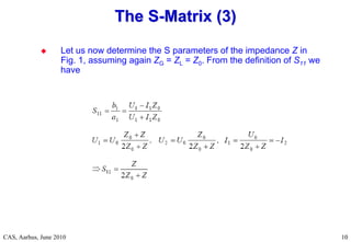
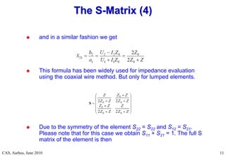
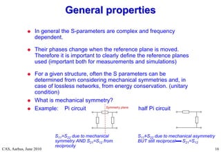
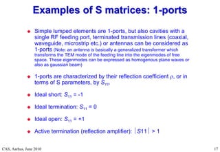
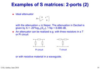
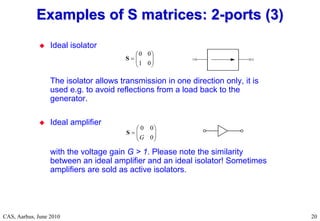
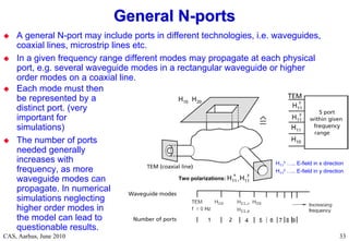
This document discusses RF engineering concepts related to S-parameters. It provides definitions of power waves and S-matrices. The S-matrix relates incoming and outgoing voltage waves at the ports of an N-port network. It describes how S-parameters can be used to characterize 1, 2, 3 and 4 port networks. Properties of S-matrices like reciprocity and unitarity for passive networks are also covered. Transfer matrices (T-matrices) are introduced as an alternative representation for cascaded 2-port networks.
![RF Basic Concepts, Caspers, McIntosh, Kroyer
CAS, Aarhus, June 2010 5
5
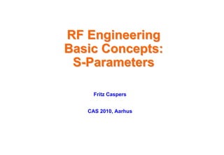
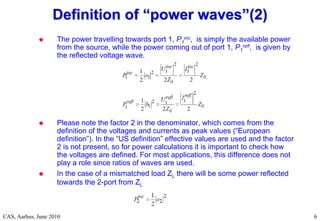
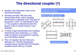
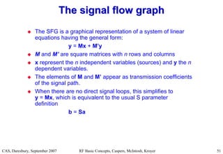
The waves going towards the n-port are a = (a1, a2, ..., an), the waves
travelling away from the n-port are b = (b1, b2, ..., bn). By definition
currents going into the n-port are counted positively and currents flowing
out of the n-port negatively. The wave a1 is going into the n-port at port 1
is derived from the voltage wave going into a matched load.
In order to make the definitions consistent with the conservation of
energy, the voltage is normalized to . Z0 is in general an arbitrary
reference impedance, but usually the characteristic impedance of a line
(e.g. Z0 = 50 ) is used and very often ZG = ZL = Z0. In the following we
assume Z0 to be real. The definitions of the waves a1 and b1 are
Note that a and b have the dimension [1].
Definition of
Definition of “
“ power waves
power waves”
”(1)
(1)](https://image.slidesharecdn.com/caspers-s-parameters-240218154803-825edc5c/85/Caspers-S-Parameters-asdf-asdf-sadf-asdf-asdf-5-320.jpg)
![RF Basic Concepts, Caspers, McIntosh, Kroyer
CAS, Aarhus, June 2010 12
12
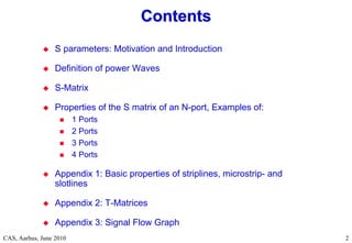
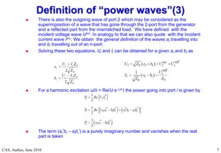
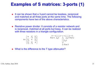
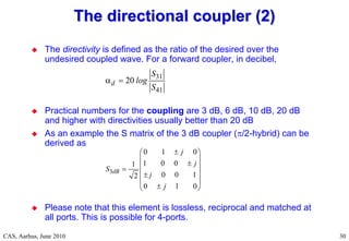
The S matrix introduced in the previous section is a very convenient way
to describe an n-port in terms of waves. It is very well adapted to
measurements and simulations. However, it is not well suited to for
characterizing the response of a number of cascaded 2-ports. A very
straightforward manner for the problem is possible with the T matrix
(transfer matrix), which directly relates the waves on the input and on
the output [2] (see appendix)
The conversion formulae between S and T matrix are given in Appendix
I. While the S matrix exists for any 2-port, in certain cases, e.g. no
transmission between port 1 and port 2, the T matrix is not defined. The
T matrix TM of m cascaded 2-ports is given by (as in [2, 3]):
Note that in the literature different definitions of the T matrix can be
found and the individual matrix elements depend on the definition used.
(see appendix)
The transfer matrix (T
The transfer matrix (T-
-matrix)
matrix)](https://image.slidesharecdn.com/caspers-s-parameters-240218154803-825edc5c/85/Caspers-S-Parameters-asdf-asdf-sadf-asdf-asdf-12-320.jpg)
![RF Basic Concepts, Caspers, McIntosh, Kroyer
CAS, Aarhus, June 2010 14
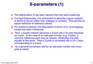
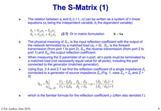
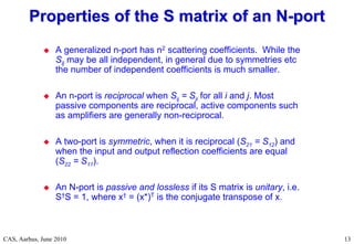
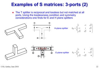
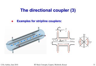
For a two-port the unitarity condition gives
which yields the three conditions
From the last equation we get, writing out amplitude and phase
and combining the equations for the modulus (amplitude)
Thus any lossless two-port can be characterized by one
amplitude and three phases.
Unitarity of an N
Unitarity of an N-
-port
port
1
0
0
1
22
21
12
11
*
22
*
12
*
21
*
11
*
S
S
S
S
S
S
S
S
S
S
T
1
1
2
22
2
12
2
21
2
11
S
S
S
S
11 12 21 22 0
* *
S S S S
22
21
12
11
22
21
12
11
arg
arg
arg
arg
and
S
S
S
S
S
S
S
S
11 22 12 21
2
11 12
1
S S , S S
S S
Note: this is a necessary but not a
sufficient condition! See next slide!
[ arg(S11) = arctan(Im(S11)/Re(S11)) ]](https://image.slidesharecdn.com/caspers-s-parameters-240218154803-825edc5c/85/Caspers-S-Parameters-asdf-asdf-sadf-asdf-asdf-14-320.jpg)
![RF Basic Concepts, Caspers, McIntosh, Kroyer
CAS, Aarhus, June 2010 18
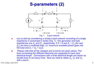
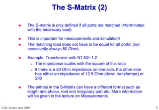
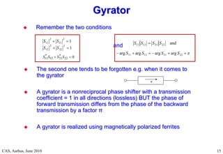
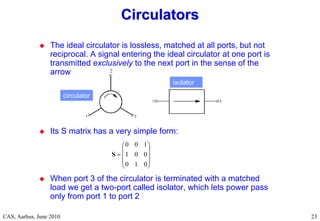
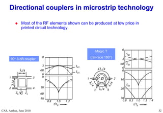
Ideal transmission line of length l
where j is the complex propagation constant, the
line attenuation in [Neper/m] and with the wavelength
. For a lossless line we get |S21| = 1.
Ideal phase shifter
For a reciprocal phase shifter , while for the gyrator
. As said before an ideal gyrator is lossless (S†S =
1), but it is not reciprocal. Gyrators are often implemented
using active electronic components, however in the
microwave range passive gyrators can be realized using
magnetically saturated ferrite elements.
Examples of S matrices: 2
Examples of S matrices: 2-
-ports (1)
ports (1)
0
0
l
l
e
e
S
0
0
21
12
j
j
e
e
S](https://image.slidesharecdn.com/caspers-s-parameters-240218154803-825edc5c/85/Caspers-S-Parameters-asdf-asdf-sadf-asdf-asdf-18-320.jpg)
![RF Basic Concepts, Caspers, McIntosh, Kroyer
References
References
CAS, Aarhus, June 2010 34
[1]
[1] K. Kurokawa, Power waves and the scattering matrix,
K. Kurokawa, Power waves and the scattering matrix,
IEEE
IEEE-
-T
T-
-MTT, Vol. 13
MTT, Vol. 13 No 2
No 2, March 1965, 194
, March 1965, 194-
-202.
202.
[2]
[2] H. Meinke, F. Gundlach, Taschenbuch der
H. Meinke, F. Gundlach, Taschenbuch der
Hochfrequenztechnik, 4. Auflage, Springer, Heidelberg, 1986,
Hochfrequenztechnik, 4. Auflage, Springer, Heidelberg, 1986,
ISBN 3
ISBN 3-
-540
540-
-15393
15393-
-4.
4.
[3]
[3] K.C. Gupta, R. Garg, and R. Chadha, Computer
K.C. Gupta, R. Garg, and R. Chadha, Computer-
-aided
aided
design of microwave circuits, Artech, Dedham, MA 1981, ISBN
design of microwave circuits, Artech, Dedham, MA 1981, ISBN
0
0-
-89006
89006-
-106
106-
-8.
8.
[4]
[4] J. Frei, X.
J. Frei, X.-
-D. Cai
D. Cai, Member, IEEE, and S. Muller,
, Member, IEEE, and S. Muller, Multiport S
Multiport S-
-
Parameter and T
Parameter and T-
-Parameter Conversion With Symmetry
Parameter Conversion With Symmetry
Extension, IEEE Transactions on Microwave Theory and
Extension, IEEE Transactions on Microwave Theory and
Techniques, VOL. 56, NO. 11, 2008, 2493
Techniques, VOL. 56, NO. 11, 2008, 2493-
-2504
2504](https://image.slidesharecdn.com/caspers-s-parameters-240218154803-825edc5c/85/Caspers-S-Parameters-asdf-asdf-sadf-asdf-asdf-34-320.jpg)
![RF Basic Concepts, Caspers, McIntosh, Kroyer
CAS, Aarhus, June 2010 37
37
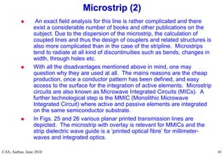
For a mathematical treatment, the effect of the fringing fields may be
described in terms of static capacities (see Fig. 20) [14]. The total
capacity is the sum of the principal and fringe capacities Cp and Cf.
Fig. 20: Design, dimensions and characteristics for offset center-conductor strip transmission line [14]
For striplines with an homogeneous dielectric the phase velocity is the
same, and frequency independent, for all TEM-modes. A
configuration of two coupled striplines (3-conductor system) may have
two independent TEM-modes, an odd mode and an even mode (Fig.
21).
Fig. 21: Even and odd mode in coupled striplines
Striplines (2)
Striplines (2)](https://image.slidesharecdn.com/caspers-s-parameters-240218154803-825edc5c/85/Caspers-S-Parameters-asdf-asdf-sadf-asdf-asdf-37-320.jpg)
![RF Basic Concepts, Caspers, McIntosh, Kroyer
CAS, Aarhus, June 2010 38
38
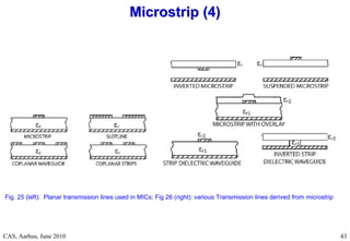
The analysis of coupled striplines is required for the design of
directional couplers. Besides the phase velocity the odd and even
mode impedances Z0,odd and Z0,even must be known. They are given as
a good approximation for the side coupled structure (Fig. 22, left).
They are valid as a good approximation for the structure shown in Fig.
22.
Striplines (3)
Striplines (3)
Fig. 22: Types of
coupled striplines [14]:
left: side coupled parallel
lines, right: broad-
coupled parallel lines](https://image.slidesharecdn.com/caspers-s-parameters-240218154803-825edc5c/85/Caspers-S-Parameters-asdf-asdf-sadf-asdf-asdf-38-320.jpg)
![RF Basic Concepts, Caspers, McIntosh, Kroyer
CAS, Aarhus, June 2010 39
39
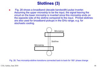
A graphical presentation of Equations 5.3 is also known as the Cohn
nomographs [14]. For a quarter-wave directional coupler (single
section in Fig. 16) very simple design formulae can be given
where C0 is the voltage coupling ratio of the /4 coupler.
In contrast to the 2-hole waveguide coupler this type couples
backwards, i.e. the coupled wave leaves the coupler in the direction
opposite to the incoming wave. The stripline coupler technology is
rather widespread by now, and very cheap high quality elements are
available in a wide frequency range. An even simpler way to make
such devices is to use a section of shielded 2-wire cable.
Striplines (4)
Striplines (4)](https://image.slidesharecdn.com/caspers-s-parameters-240218154803-825edc5c/85/Caspers-S-Parameters-asdf-asdf-sadf-asdf-asdf-39-320.jpg)
![RF Basic Concepts, Caspers, McIntosh, Kroyer
CAS, Aarhus, June 2010 42
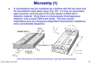
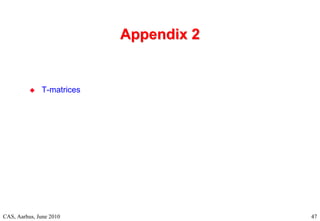
Microstrip (3)
Microstrip (3)
Fig. 24: Characteristic impedance (current/power definition) and effective permittivity of a microstrip line [16]
](https://image.slidesharecdn.com/caspers-s-parameters-240218154803-825edc5c/85/Caspers-S-Parameters-asdf-asdf-sadf-asdf-asdf-42-320.jpg)


![RF Basic Concepts, Caspers, McIntosh, Kroyer
CAS, Aarhus, June 2010 48
The T matrix (transfer matrix), which directly relates the waves on the
input and on the output, is defined as [2]
As the transmission matrix (T matrix) simply links the in- and outgoing
waves in a way different from the S matrix, one may convert the matrix
elements mutually
The T matrix TM of m cascaded 2-ports is given by a matrix multiplication
from the ‘left’ to the right as in [2, 3]:
T
T-
-Matrix
Matrix
1 11 12 2
1 21 22 2
b T T a
a T T b
22 11 11
11 12 12
21 21
22
21 22
21 21
1
S S S
T S , T
S S
S
T , T
S S
m
2
1
M T
T
T
T
](https://image.slidesharecdn.com/caspers-s-parameters-240218154803-825edc5c/85/Caspers-S-Parameters-asdf-asdf-sadf-asdf-asdf-48-320.jpg)
![RF Basic Concepts, Caspers, McIntosh, Kroyer
CAS, Aarhus, June 2010 49
There is another definition that takes a1 and b1 as independent variables.
and for this case
Then, for the cascade, we obtain
i.e. a matrix multiplication from ‘right’ to ‘left’.
Note that there is no standardized definition of the T-matrix [4]
T
T-
-Matrix
Matrix
2 11 12 1
2 1
21 22
b T T a
a b
T T
22 11 22
11 21 12
12 12
11
21 22
12 12
1
S S S
T S , T
S S
S
T , T
S S
1
1
~
~
~
~
T
T
T
TM
m
m](https://image.slidesharecdn.com/caspers-s-parameters-240218154803-825edc5c/85/Caspers-S-Parameters-asdf-asdf-sadf-asdf-asdf-49-320.jpg)


![RF Circuit Design - [Ch3-2] Power Waves and Power-Gain Expressions](https://cdn.slidesharecdn.com/ss_thumbnails/ch3-2-150613064404-lva1-app6891-thumbnail.jpg?width=640&height=640&fit=bounds)


![RF Circuit Design - [Ch3-1] Microwave Network](https://cdn.slidesharecdn.com/ss_thumbnails/ch3-1-150613064402-lva1-app6892-thumbnail.jpg?width=640&height=640&fit=bounds)


