![202 4 The Double Multi-Layer Potential Operator
we conclude
!m
X mŠ X
n
2˛
D 2
k D j j2m ; 8 2 Rn ; (4.19)
˛Š
j˛jDm kD1
so (4.16) reduces to (4.15) when j WD ˛ Áj with 2 Rn and Á D .Áj /1Äj ÄM 2
˛
CM .
Finally, we remark that we will occasionally require only a much weaker
condition than (4.16), namely the semi-positivity condition to the effect
that
0 1
X X ˛ˇ
M
Re @ aj k j k A 0; 8 j 2 C; j˛j D m; 1 Ä j Ä M: (4.20)
˛ ˇ ˛
j˛jDjˇjDm j;kD1
We wish to note that given a differential operator L D LA as in (4.1),
corresponding to some tensor coefficient A D A˛ˇ j˛jDjˇjDm , there exist infinitely
many other tensor coefficients B D B˛ˇ j˛jDjˇjDm such that L D LB . In turn, the
choice of these B’s may affect some of the properties of the operator L discussed
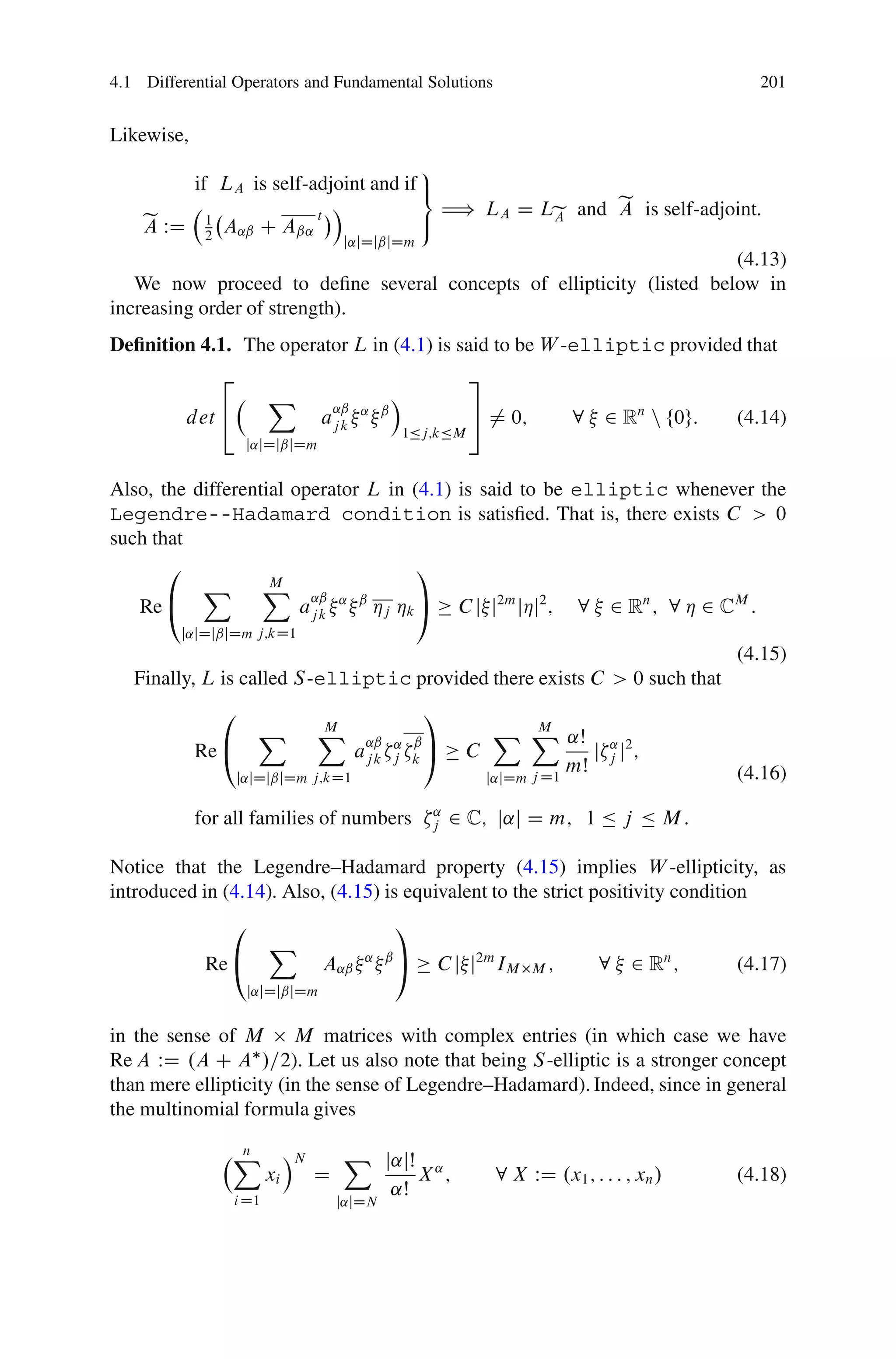
above. Concretely, while the quality of being W-elliptic (cf. (4.14)) or satisfying
the Legendre–Hadamard condition (4.15) are unaffected by the choice of tensor
coefficient B used in the writing of the given operator L, the property of being
S-elliptic (cf. (4.16)) and the semi-positivity condition (4.20) may fail for LB .
A few examples of homogeneous, constant coefficient, higher-order elliptic
operators are as follows. First, the polyharmonic operator
X mŠ
m
D @2 ; (4.21)
Š
j jDm
has been extensively studied in the literature. In the three-dimensional setting, the
fourth order operator
@4 C @4 C @4
1 2 3 (4.22)
has been considered by I. Fredholm who has computed an explicit fundamental
solution for it in [48]. More generally, an explicit fundamental solution for the
operator
@4 C @4 C @4 C c @2 @2 C @2 @2 C @2 @2
1 2 3 1 2 1 3 2 3 (4.23)
which is elliptic if c 2 . 1 ; 1/ has been found in [130] (where elliptic operators
P 2
of the form 3 2 2
j;kD1 aj k @j @k have also been considered).](https://image.slidesharecdn.com/multi-layerpotentialsandboundaryproblems-130326071052-phpapp01/75/Multi-layer-potentials-and-boundary-problems-4-2048.jpg)
![4.1 Differential Operators and Fundamental Solutions 203
Moving on, recall that the classical Malgrange–Ehrenpreis theorem asserts that
P
any differential operator of the form P .@/ D j˛jÄm a˛ @ , with a˛ 2 C not all
˛
0
zero, has a fundamental solution E 2 D .R / in R . In fact, as noted in [100], one
n n
may take
Z
1 P .i C zÁ/ Á d z
E.X / WD zm e zhÁ;X i F 1
!X : (4.24)
2 i Pm .Á/ z2C; jzjD1 P .i C zÁ/ z
Above, F !X is the inverse of the Fourier transform, originally defined by the
1
R
formula FX ! . / WD Rn e i hX; i .X / dX for 2 Cc1 .Rn / and
P 2 Rn ,
then extended by continuity to tempered distributions. Also, P . / D j˛jÄm a˛ ˛ ,
2 Cn , is the characteristic polynomial of P .@/, and Pm stands for the principal
part of P . Finally, Á 2 Cn is a fixed vector with the property that Pm .Á/ 6D 0.
We shall need a result of a somewhat similar nature for systems of differential
operators. The theorem below is essentially a collection of results proved in [60,
pp. 72–76], [57, p. 169], [114], and [95, p. 104], in various degrees of generality.
However, we feel that it is useful to have a unifying statement, accompanied by a
fairly self-contained proof, presented here.
Theorem 4.2. Let L be a homogeneous differential operator L in Rn of order 2m,
m 2 N, with complex matrix-valued constant coefficients as in (4.1) which satisfies
(4.14). Then, there exists a matrix of tempered distributions, E D Ej k 1Äj;kÄM ,
such that the following hold:
(1) For each 1 Ä j; k Ä M ,
Ej k 2 C 1 .Rn n f0g/ and Ej k . X / D Ej k .X / 8 X 2 Rn n f0g: (4.25)
(2) For each 1 Ä j; k Ä M ,
(
X
M h i 0 if j ¤ k;
LX
jr Erk .X Y/ D (4.26)
rD1 ıY .X / if j D k;
where ı stands for the Dirac delta distribution at 0 and the superscript X
denotes the fact that the operator Ljs in (4.26) is applied in the variable X .
(3) If 1 Ä j; k Ä M , then
Á
Ej k .X / D ˚j k .X / C log jX j Pj k .X /; X 2 Rn n f0g; (4.27)
where ˚j k 2 C 1 .Rn n f0g/ is a homogeneous function of degree 2m n, and
Pj k is identically zero when either n is odd, or n > 2m, and is a homogeneous
polynomial of degree 2m n when n Ä 2m. In fact,](https://image.slidesharecdn.com/multi-layerpotentialsandboundaryproblems-130326071052-phpapp01/75/Multi-layer-potentials-and-boundary-problems-5-2048.jpg)
![204 4 The Double Multi-Layer Potential Operator
Á Z X Á
1 1
Pj k .X/ D .X /2m n ˛Cˇ
A˛ˇ d
1Äj;kÄM .2 i/n .2m n/Š
Sn 1 j˛jDjˇjDm
(4.28)
for X 2 Rn .
(4) For each ˛ 2 Nn there exists C˛ > 0 such that
0
8 C˛
ˆ
ˆ if either n is odd, or n > 2m, or if j˛j > 2m n;
ˆ jXjn 2mCj˛j
<
j@ E.X/j Ä
˛
ˆ C .1 C j log jXjj/
ˆ ˛
ˆ
: if 0 Ä j˛j Ä 2m n;
jXjn 2mCj˛j
(4.29)
uniformly for X 2 Rn n f0g.
(5) One can assign to each differential operator L as in (4.1)–(4.14) a fundamental
solution EL which satisfies (1)-(4) above and, in addition,
t
EL D ELt ; EL D EL ; EL D EL : (4.30)
(6) The matrix-valued distribution E has entries which are tempered distributions
b
in Rn . When restricted to Rn n f0g, the matrix-valued distribution E (with
1
“hat” denoting the Fourier transform, defined as before) is a C function and,
moreover,
X Á 1
b
E. / D . 1/m ˛Cˇ
A˛ˇ for each 2 Rn n f0g: (4.31)
j˛jDjˇjDm
(7) For each multi-index ˛ 2 Nn with j˛j D 2m 1, the function @˛ E is odd, C 1
0
smooth, and homogeneous of degree n 1 in Rn n f0g.
Proof. Let P j k . / 1Äj;kÄM
be the inverse of the characteristic matrix
X
L. / WD A˛ˇ ˛Cˇ
; 2 Rn n f0g: (4.32)
j˛jDjˇjDm
Following [60, p. 76], if n is odd, define
Z h i
1 .n 1/=2
Ej k .X / WD n 1 .2m X .X /2m 1
sign .X / P j k . / d ;
4.2 i / 1/Š
Sn 1
(4.33)
for X 2 Rn n f0g. Note that this expression is homogeneous of degree 2m n. On
the other hand, if n is even, set](https://image.slidesharecdn.com/multi-layerpotentialsandboundaryproblems-130326071052-phpapp01/75/Multi-layer-potentials-and-boundary-problems-6-2048.jpg)
![4.1 Differential Operators and Fundamental Solutions 205
Z h i
1 n=2
Ej k .X / WD X .X /2m log jX j P jk. / d ; (4.34)
.2 i /n .2m/Š Sn 1
where X 2 Rn n f0g. It is also clear from (4.33)–(4.34) that E is an even function.
Alternatively, transferring one Laplacian under the integral sign when n is odd,
Á
using the fact that log Xi D log jX j i
2 sign .X / and simple parity
considerations, it can be checked that
Z h
1 .nCq/=2 X Ái j k
Ej k .X / D .X /2mCq log P . /d ;
.2 i /n .2m C q/Š X i
Sn 1
(4.35)
for X 2 Rn n f0g, where q WD 0 if n is even and q WD 1 if n is odd.
As a preamble to checking (4.26), consider F .t/ WD t 2mCq log .t= i /, t 2 R n f0g,
and note that there exists a constant Cm;q such that
d Á2m .2m C q/Š q t
F .t/ D t log C Cm;q t q : (4.36)
dt qŠ i
Consequently,
h .2m C q/Š X i
LX F .X /D .X /q log C Cm;q .X /q L. / (4.37)
qŠ i
and, further,
Z h Ái Á
1 X
LX n .2m C q/Š
.X /2mCq log ŒL. / 1
d
.2 i / Sn 1 i
Á
D B.nCq/=2 .X / C Pq .X / IM M; (4.38)
where
Z Á
1 X
B.nCq/=2 .X / WD .X /q log d (4.39)
.2 i /n qŠ Sn 1 i
is a fundamental solution for .nCq/=2 (cf., e.g., Lemma 4.2 on p. 123 in [122]),
Pq .X / is a homogeneous polynomial of degree q, and IM M is the identity matrix.
.nCq/=2
Applying X to both sides of (4.38) then gives
LE D ı IM M (4.40)
i.e., (4.26) holds.](https://image.slidesharecdn.com/multi-layerpotentialsandboundaryproblems-130326071052-phpapp01/75/Multi-layer-potentials-and-boundary-problems-7-2048.jpg)
![4.2 The Definition of Double Multi-Layer and Non-tangential Maximal Estimates 207
Let us observe that, thanks to S (4.45)–(4.47), «j k is actually a smooth,
unambiguously defined function in n O` D Rn n f0g. In particular, the decom-
`D1
position (4.27) follows from the above discussion in concert with (4.45) and (4.35).
Concerning (4.28), we first observe that
Z
1 .nCq/=2
Pj k .X / D .X /2mCq P j k . / d ; (4.48)
.2 i /n .2m C q/Š X Sn 1
as seen from (4.35), (4.27), (4.45)–(4.46), and the identity
NŠ
K
X Œ.X /N D .X /N 2K
j j2K ; (4.49)
.N 2K/Š
valid for any N; K 2 N with N 2K.
The estimates in (4.29) are a direct consequence of the structure formula (4.27).
Finally, (4.33)–(4.34) readily account for the transposition identity (4.30).
The proof of (6) relies on (4.27) which we shall abbreviate as E D ˚ C « , where
we have set ˚.X / WD ˚j k .X / j;k and « .X / WD log jX j Pj k .X / j;k . First, we
note that ˚ 2 C 1 .Rn n f0g/ L1 .Rn / is a homogeneous function and so, by
loc
Theorem 7.1.18 on p. 168 of [57], ˚ is a (matrix-valued) tempered distribution
b
in Rn whose Fourier transform ˚ coincides with a C 1 function on Rn n f0g. As
for « , pick a function  2 Cc1 .B.0; 2// such that  Á 1 on B.0; 1/ and write
« D «1 C «2 with «1 WD .1 Â/« 2 C 1 .Rn /, a matrix-valued tempered
b
distribution, and «2 WD « 2 L1 .Rn /. Hence, « 2 2 C 1 .Rn /. Also, for every
comp
multi-index ˇ 2 N0 , the function X @ «1 .X / belongs to L1 .Rn / if ˛ 2 Nn is
n ˇ ˛
0
such that j˛j is large enough. This readily implies that for any k 2 N there exists
b b
˛ 2 Nn such that @˛ «1 2 C k .Rn /. Thus, the function Rn 3 7! ˛ « 1 . / belongs
0
k n b1 2 C 1 .Rn n f0g/.
to C .R / if j˛j is large enough, relative to k, forcing «
The above reasoning shows that E is a matrix-valued tempered distribution in
b
Rn with E a function of class C 1 , when restricted to Rn n f0g. Having established
b
this, taking the Fourier transforms of both sides of (4.40) gives . 1/m L. /E. / D
IM M in the sense of tempered distributions in R . Restricting this identity to
n
Rn n f0g gives (4.31).
Finally, the claim in part .7/ is a direct consequence of (1) and (3), and this
completes the proof of Theorem 4.2. t
u
4.2 The Definition of Double Multi-Layer and
Non-tangential Maximal Estimates
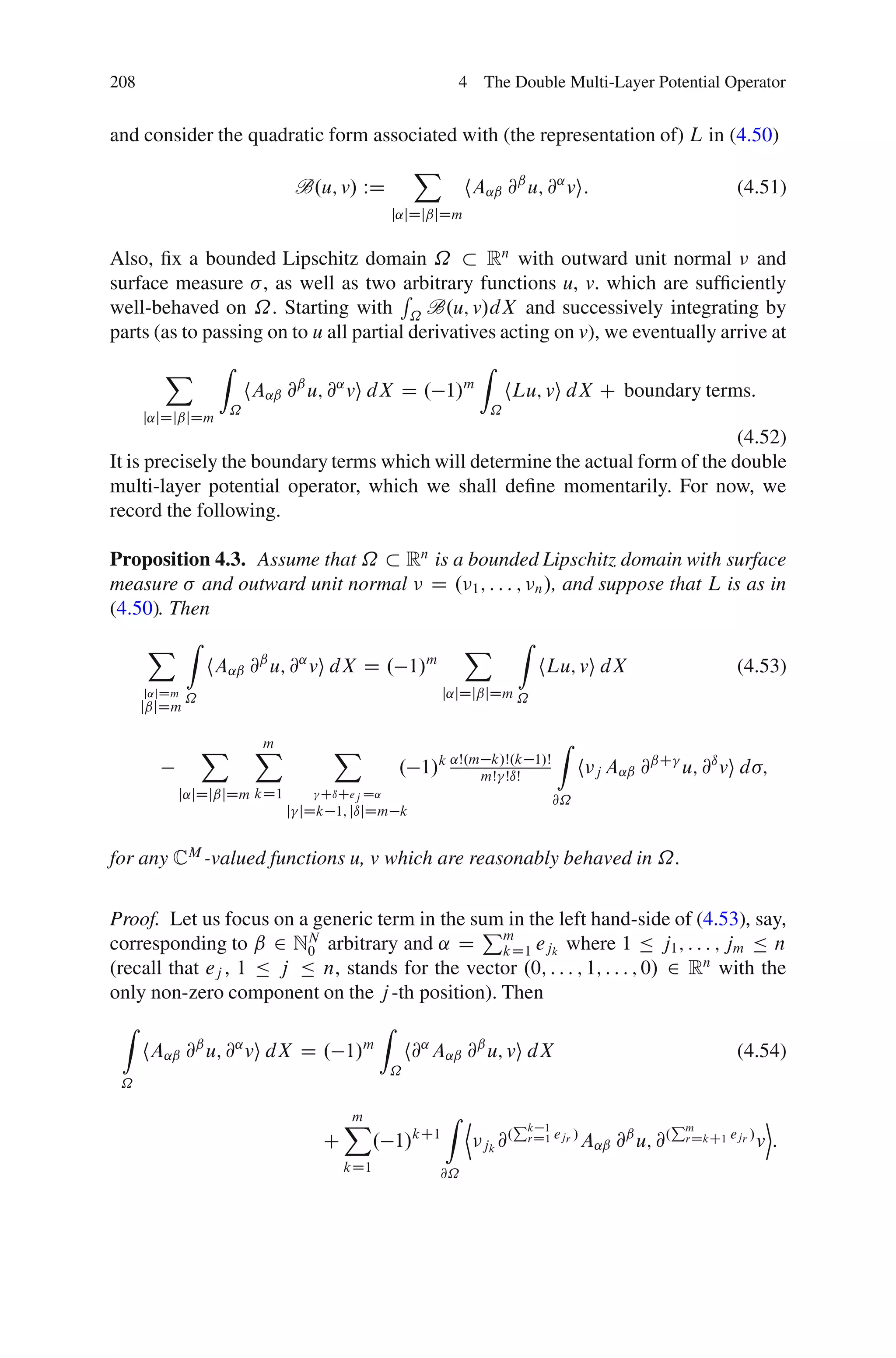
Let L be a homogeneous differential operator of order 2m, with constant (possibly
matrix-valued) coefficients:
X
L WD @˛ A˛ˇ @ˇ (4.50)
j˛jDjˇjDm](https://image.slidesharecdn.com/multi-layerpotentialsandboundaryproblems-130326071052-phpapp01/75/Multi-layer-potentials-and-boundary-problems-9-2048.jpg)
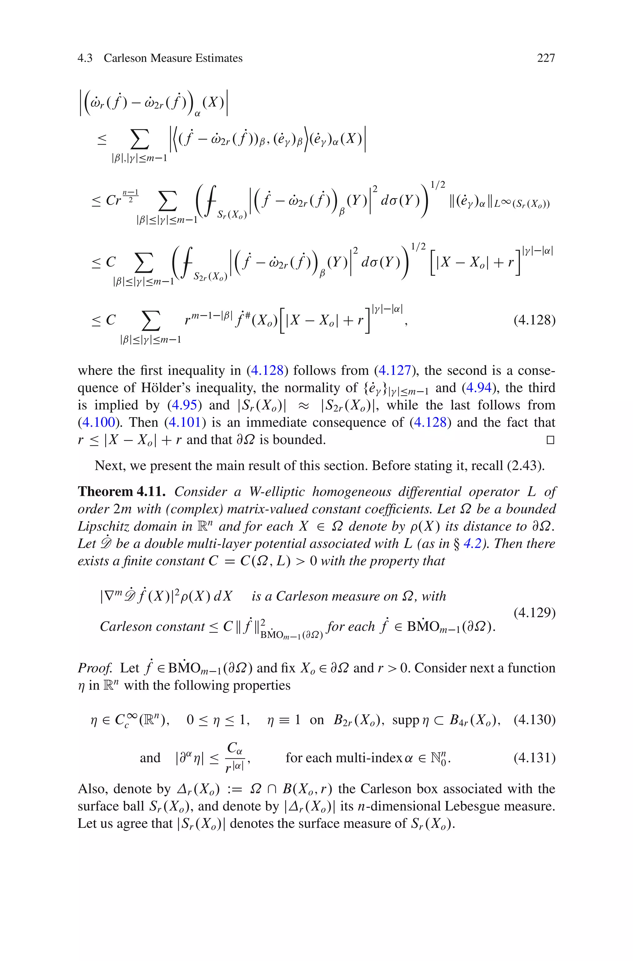
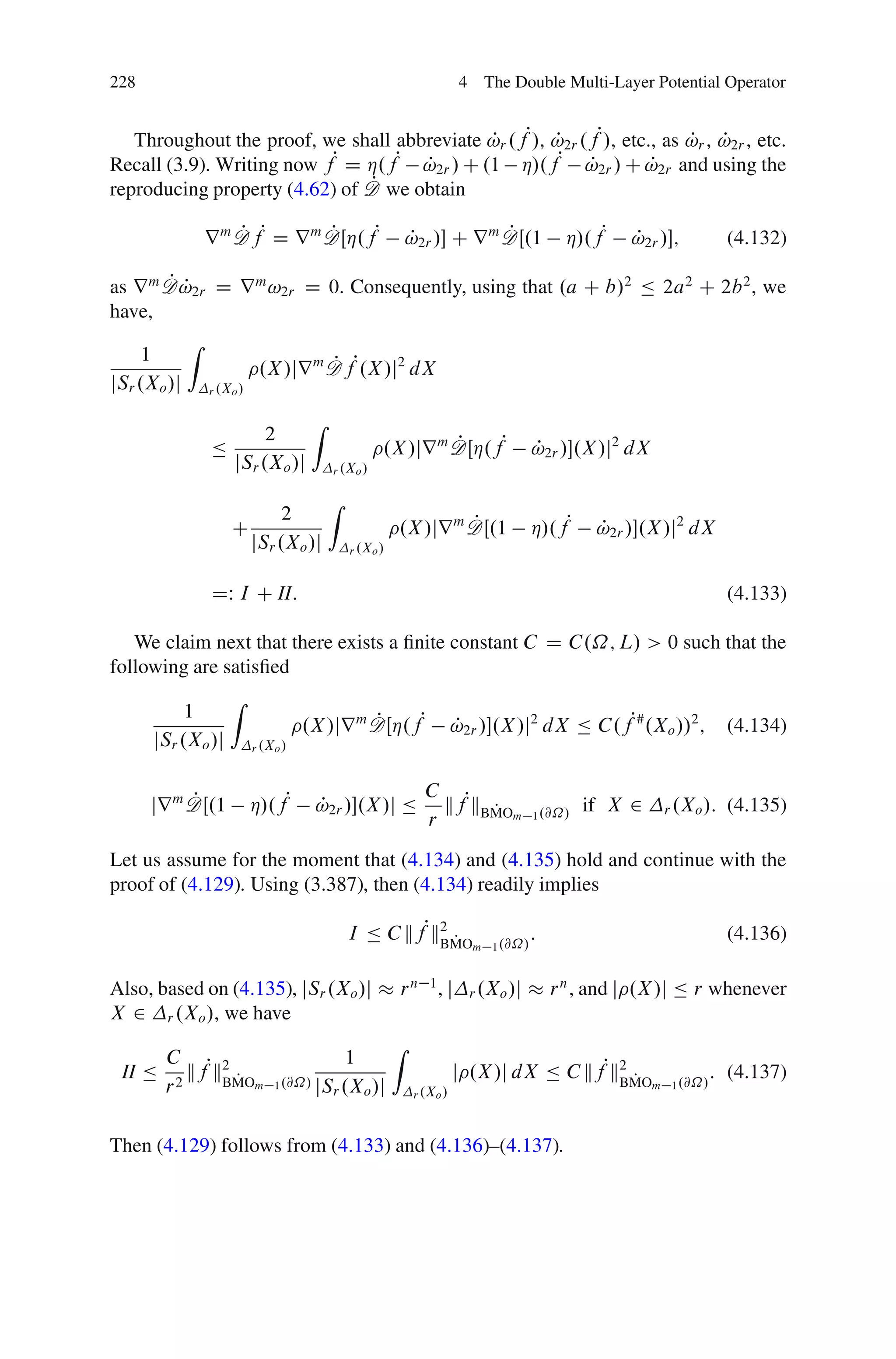
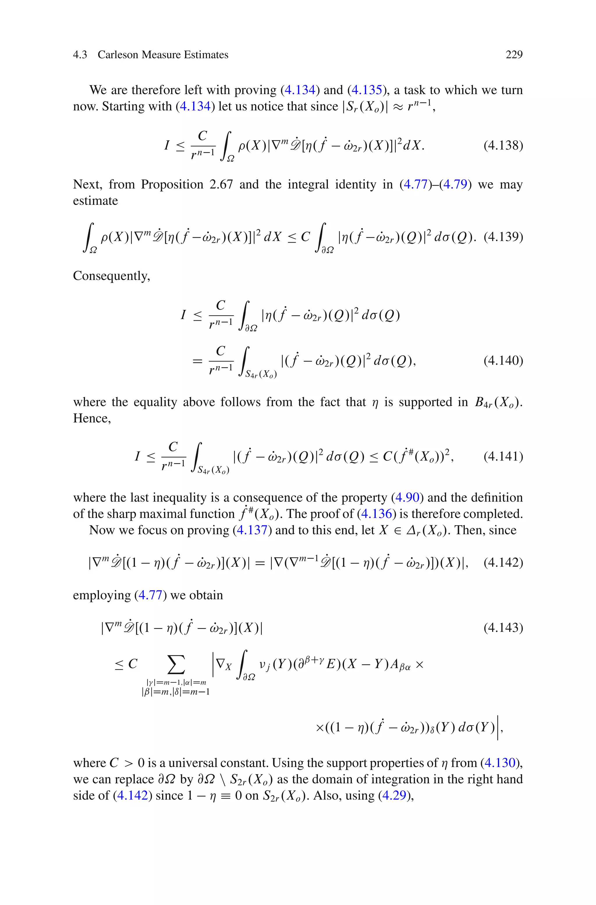
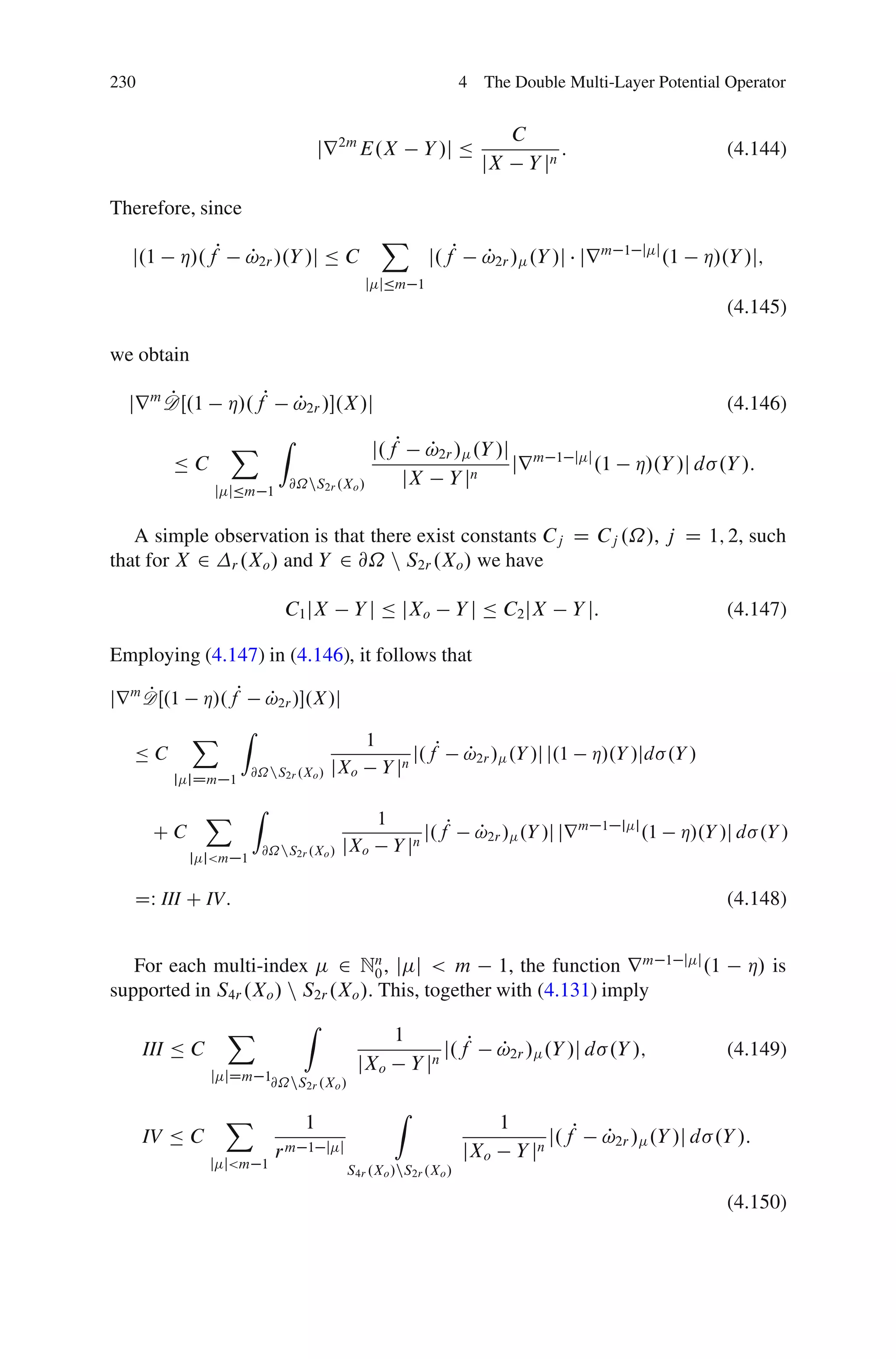
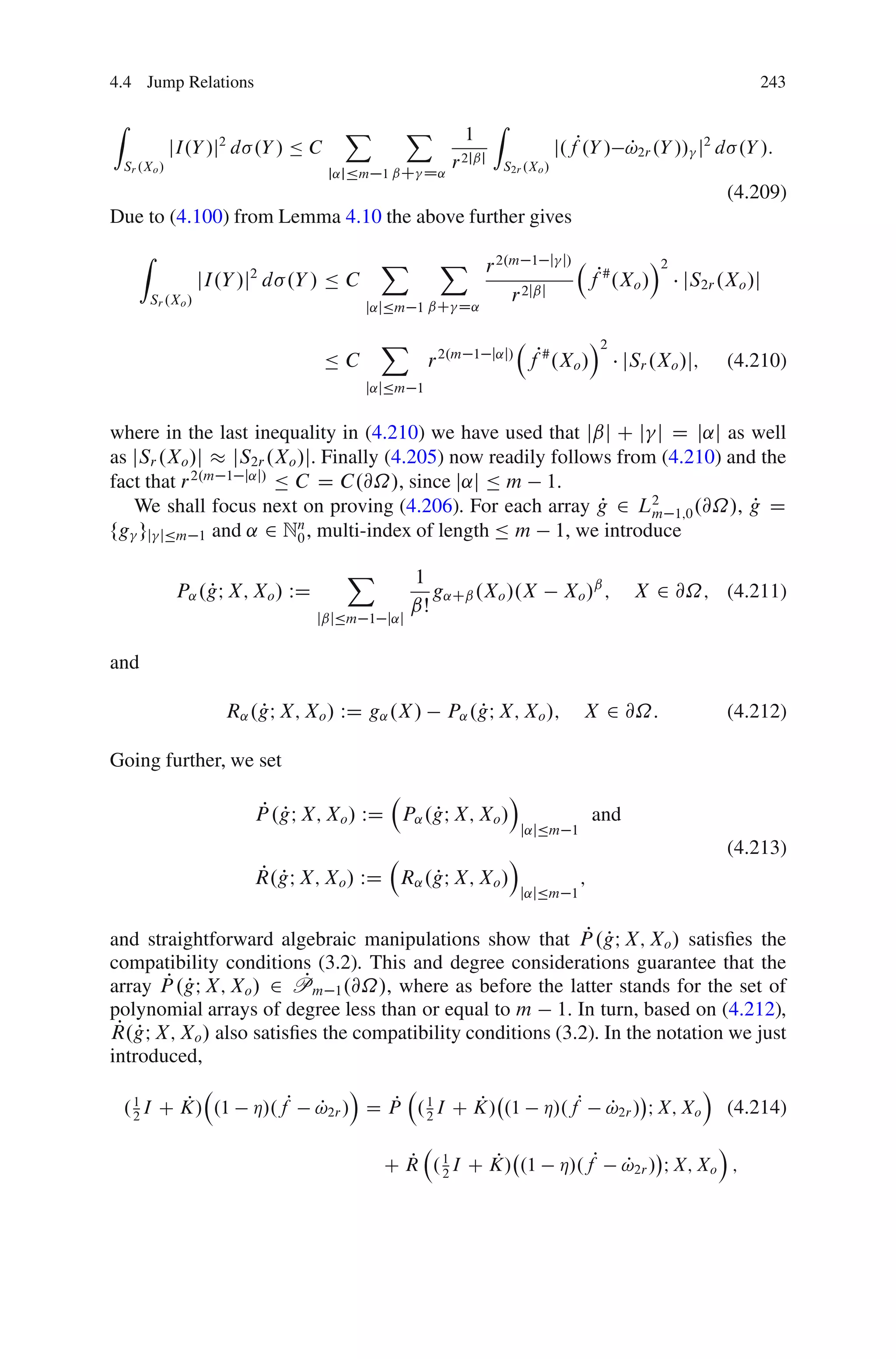
![4.3 Carleson Measure Estimates 221
In the sequel, we shall frequently identify a generic element fP from Pm 1 .Sr .Xo //
P
with its canonical extension to the entire boundary @˝. By definition, the latter is
P
taken to be trm 1 P 2 Pm 1 .@˝/, where P 2 Pm 1 is the polynomial extension to
Rn of fP. We emphasize that, by design, the canonical extension of elements from
P P
Pm 1 .Sr .Xo // to elements in Pm 1 .@˝/ is unique.
P
The space Pm 1 .Sr .Xo // has a Hilbert structure when equipped with the inner
product naturally inherited from L2 .Sr .Xo // ˚ ˚ L2 .Sr .Xo //, N times (with
N as in (4.89)). Then, given (4.93), the restrictions to Sr .Xo / of the Whitney
P
arrays p˛ .X / WD trm 1 Œ.X Xo /˛ , ˛ 2 Nn with j˛j Ä m 1, form a basis in
0
P P m 1 .Sr .Xo //. Applying the Gram–Schmidt process to fp˛ gj˛jÄm 1 then yields an
P
P
orthonormal (relative to L2 .Sr .Xo // ˚ ˚ L2 .Sr .Xo //) basis for Pm 1 .Sr .Xo //.
We denote this basis by fe˛ gj˛jÄm 1 and, for each multi-index ˛ 2 Nn of length Ä
P 0
m 1, we let e˛ 2 Pj˛j be the polynomial extension to Rn of e˛ . That is, e˛ is a
P
polynomial of degree j˛j such that e˛ D Œtrm 1 e˛ jSr .Xo / . Then, for each ˇ 2 Nn ,
P 0
jˇj Ä m 1, it follows that at points in Sr .Xo /
P
.e˛ /ˇ D .trm 1 e˛ /ˇ D @ˇ e˛ D 0 if jˇj > j˛j; (4.94)
by degree considerations. Also, by carefully keeping track of bounds for the
various expressions appearing in the Gram–Schmidt orthonormalization process (as
presented on, e.g., p. 120 of [121]) we obtain
C h ij˛j jˇj
j.e˛ /ˇ .X /j Ä
P jX Xo j C r if jˇj Ä j˛j; 8 X 2 @˝: (4.95)
r .n 1/=2
The point of the above considerations is to facilitate discussing a number of
important properties of the best fit polynomial array (cf. (4.88)). To begin with,
we agree that !r .fP/ is always identified with its canonical extension to @˝. Thus,
P
!r .fP/ 2 Pm 1 .@˝/;
P P 8 fP 2 L2
Pm 1;0 .@˝/: (4.96)
Let us also observe that
!r .fP/ D fP;
P 8 fP 2 Pm 1 .@˝/;
P (4.97)
since, by definition, !r .fP/ coincides with fPjSr .Xo / and any fP 2 Pm 1 .@˝/ is the
P P
canonical extension of fPjSr .Xo / . As an immediate corollary of (4.96)–(4.97), we
note that
!r .!2r .fP// D !2r .fP/;
P P P 8 fP 2 L2
Pm 1;0 .@˝/: (4.98)
Finally, for each fP D ffˇ gjˇjÄm 1
P
2 L2m 1;0 .@˝/, we have
X
!r .fP/ D
P hfˇ ; .e˛ /ˇ i e˛
P P on @˝; (4.99)
j˛j;jˇjÄm 1](https://image.slidesharecdn.com/multi-layerpotentialsandboundaryproblems-130326071052-phpapp01/75/Multi-layer-potentials-and-boundary-problems-23-2048.jpg)
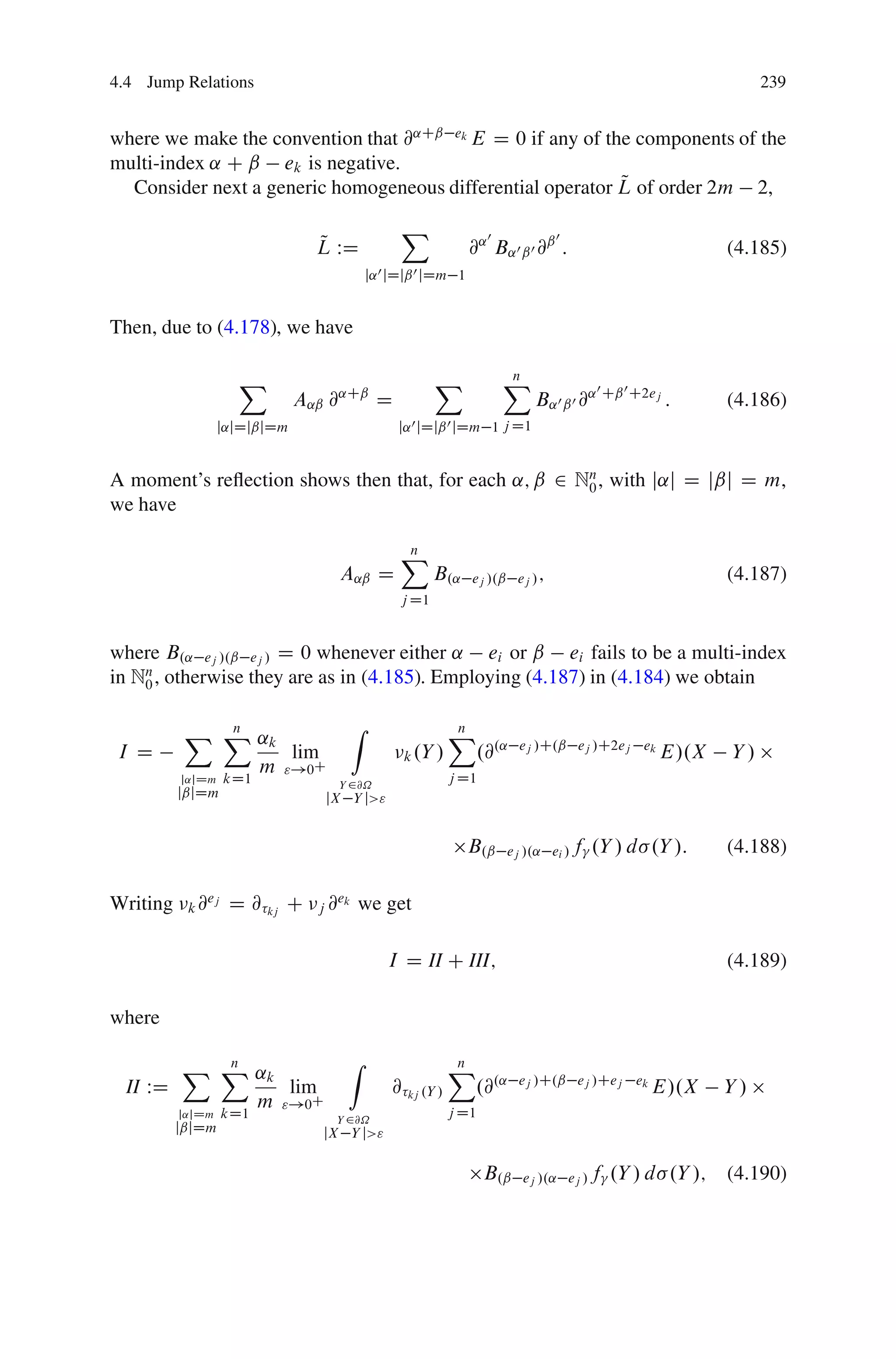
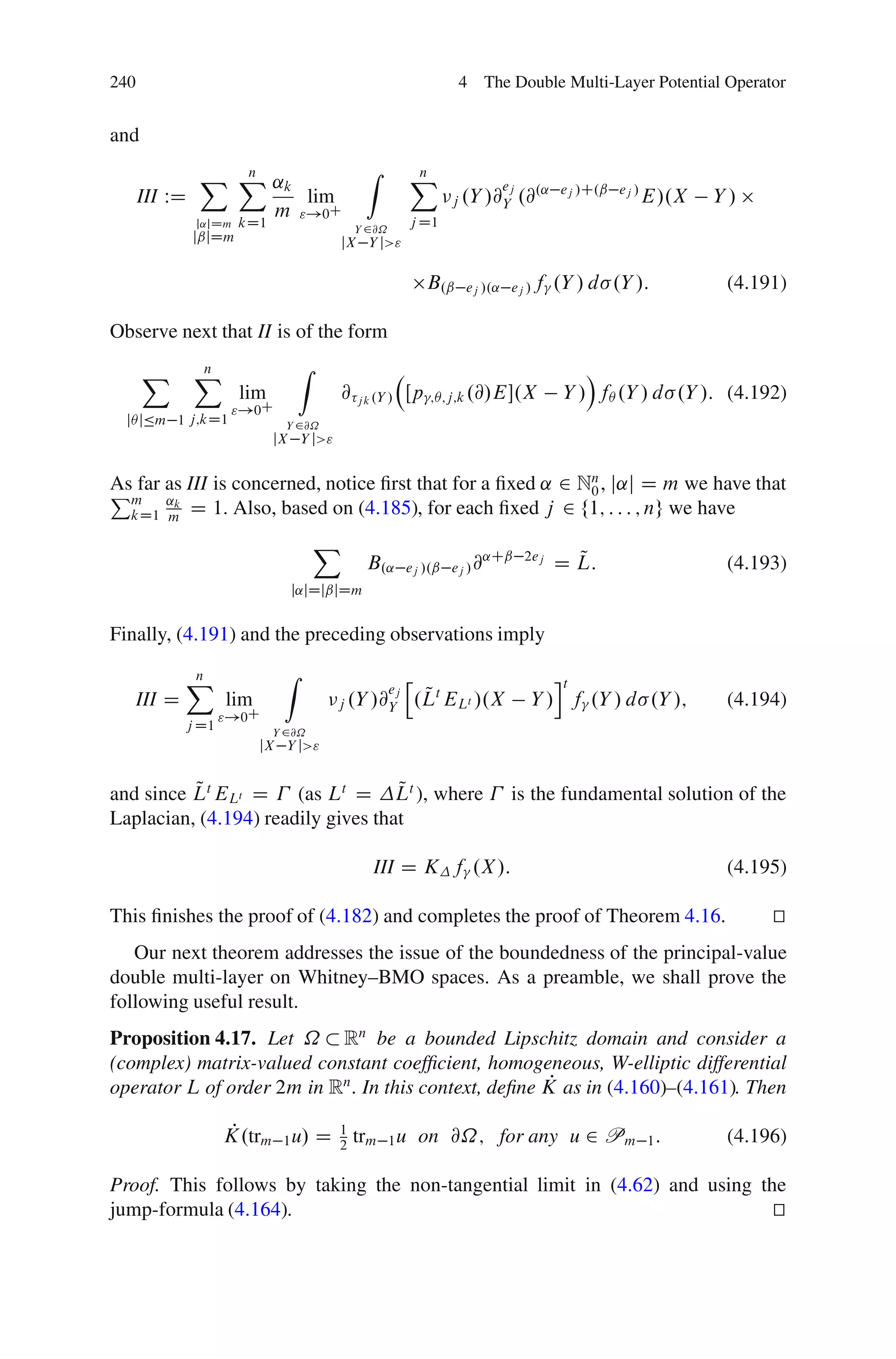
![4.4 Jump Relations 241
The action of the principal-value double multi-layer on Whitney–BMO spaces is
considered next. The theorem below extends work done in the case when n D 2 and
L D 2 in [24] and answers the question posed by J. Cohen at the top of page 111
in [24].
Theorem 4.18. Assume that ˝ Rn is a bounded Lipschitz domain, L is a
(complex) matrix-valued constant coefficient, homogeneous, W-elliptic differential
P
operator L of order 2m in Rn , and consider K as in (4.160)–(4.161). Then
P P P
K W BMOm 1 .@˝/ ! BMOm 1 .@˝/; (4.197)
is well-defined, linear and bounded.
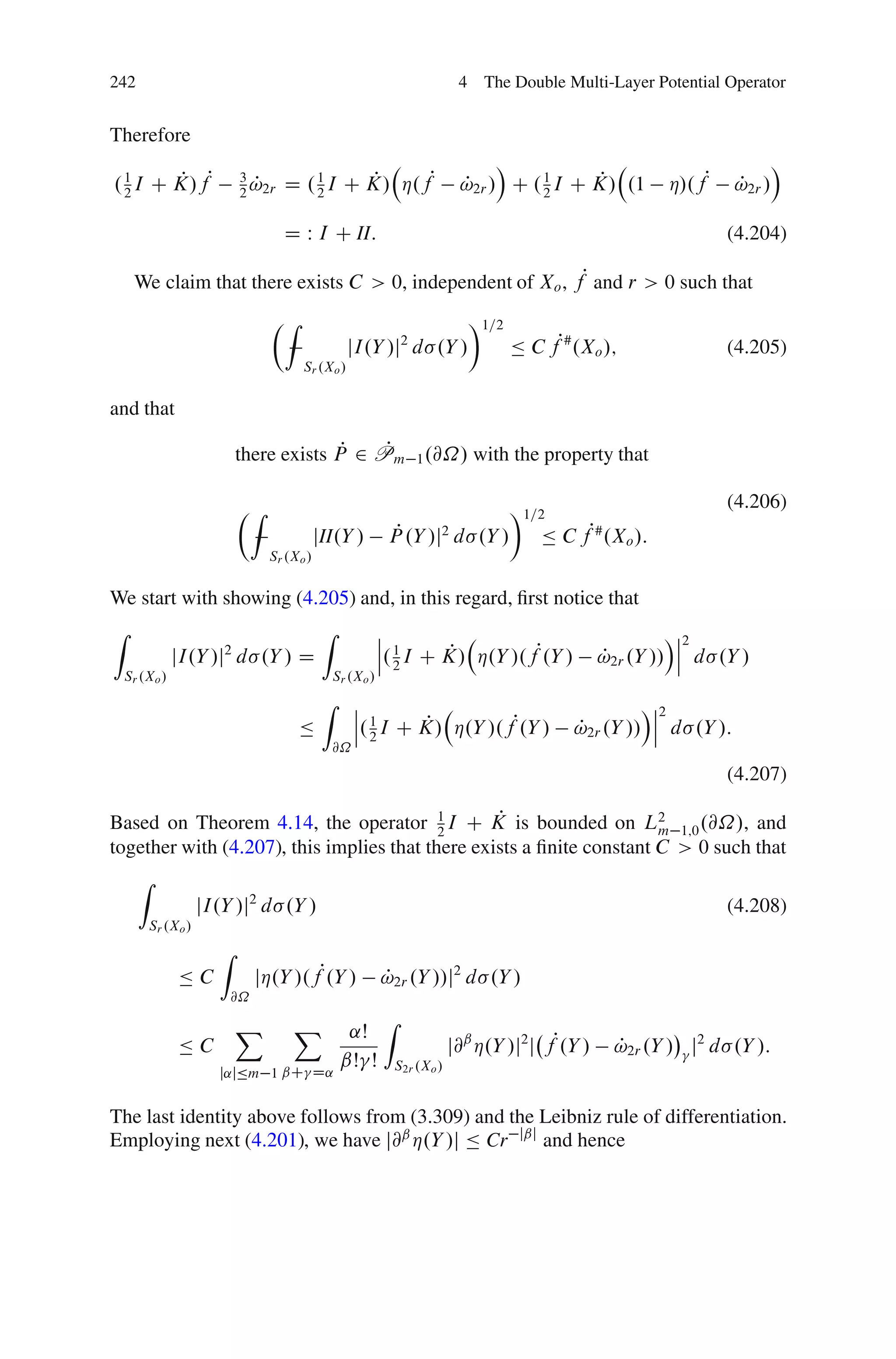
Proof. The first observation is that, given an arbitrary fP 2 BMOm 1 .@˝/, due to
P
(4.163),
K fP 2 L2
P Pm 1;0 .@˝/: (4.198)
Therefore matters reduce to showing
.K fP/# 2 L1 .@˝/:
P (4.199)
To this end, fix Xo 2 @˝, r > 0 and fP 2 BMOm 1 .@˝/. For each R > 0, recall the
P
P
best fit polynomial array !R .f P/ introduced as in (4.88). We consider next a function
Á in Rn as in (4.130). In particular the following hold
Á 2 Cc1 .Rn /; 0 Ä Á Ä 1; Á Á 1 on S2r .Xo /; suppÁ S4r .Xo /; (4.200)
C˛
j@˛ Áj Ä ; for each ˛ 2 Nn :
0 (4.201)
r j˛j
We write
fP D Á.fP !2r / C .1
P Á/.fP !2r / C !2r ;
P P (4.202)
P P
where for an array g, the multiplication Ág is in the sense of (3.309). Using the
P
linearity of the operator K on L2 1;0 .@˝/, formulas (4.202) and (4.196) give
m
Á
1
2
I C K fP D
P 1
2
I P
CK Á.fP P
!2r /
Á
C 1I C K
2
P .1 Á/.fP !2r / C 3 !2r :
P 2
P (4.203)](https://image.slidesharecdn.com/multi-layerpotentialsandboundaryproblems-130326071052-phpapp01/75/Multi-layer-potentials-and-boundary-problems-43-2048.jpg)
![4.5 Estimates on Besov, Triebel–Lizorkin, and Weighted Sobolev Spaces 247
matters can be reduced to considering the case when p D q D 1. To this end, let
us fix fP D ffÁ gjÁjÄm 1 2 Bm 1;s .@˝/ of norm one, and abbreviate (4.4) as
P 1;1
X Z
D fP.X/ D
P ˛;ˇ
C ;Á;j j .Y /.@ˇC E/.X Y /Aˇ˛ fÁ .Y / d .Y /; X 2 ˝;
j˛jDjˇjDm
@˝
CÁCej D˛
(4.232)
˛;ˇ
where the C ;Á;j ’s are real constants. For each multi-index 2 Nn of length Ä m 1,
0
consider next, in analogy with (3.78) and (3.73),
X 1
P .X; Y / WD fıC .Y /.X Y /ı ; X 2 Rn ; Y 2 @˝; (4.233)
ıŠ
jıjÄm 1 j j
R .X; Y / WD f .X / P .X; Y /; X; Y 2 @˝: (4.234)
For ease of reference, for each Y 2 @˝ let us also set
P
P . ; Y / WD fP . ; Y /gj jÄm 1 ;
P
R. ; Y / WD fR . ; Y /gj jÄm 1 : (4.235)
P
A direct calculation shows that P . ; Y / 2 C C for every Y 2 @˝ (cf. (3.81), or the
discussion on p. 177 in [119]). Since f .X / D P .X; Z/CR .X; Z/ if j j Ä m 1
and X; Z 2 @˝, we have
fP D P . ; Z/ C R. ; Z/;
P P 8 Z 2 @˝: (4.236)
P P
In particular, R. ; Y / 2 C C for every Y 2 @˝. Furthermore, since P . ; Z/ D
has polynomial components of degree Ä m 1, it follows from (4.236) and the
reproducing property (4.62) that
D fP.X / D D.P . ; Z//.X / C D.R. ; Z//.X /
P P P P P
P P
D P.0;:::;0/ .X; Z/ C D.R. ; Z//.X / (4.237)
for every X 2 ˝ and Z 2 @˝. Consequently, for each multi-index  2 Nn with
0
jÂj D m, we arrive at the identity
@Â D fP.X / D @Â D.R. ; Z//.X /
P P P (4.238)
X Z
˛;ˇ ˇC CÂ
D C ;Á;j j .Y /.@ E/.X Y /Aˇ˛ RÁ .Y; Z/ d .Y /;
j˛jDjˇjDm
@˝
CÁCej D˛
valid for each X 2 ˝ and Z 2 @˝. Next, given a point X 2 ˝, we specialize
(4.238) by choosing Z WD .X /, where W ˝ ! @˝ is a mapping chosen with the](https://image.slidesharecdn.com/multi-layerpotentialsandboundaryproblems-130326071052-phpapp01/75/Multi-layer-potentials-and-boundary-problems-49-2048.jpg)


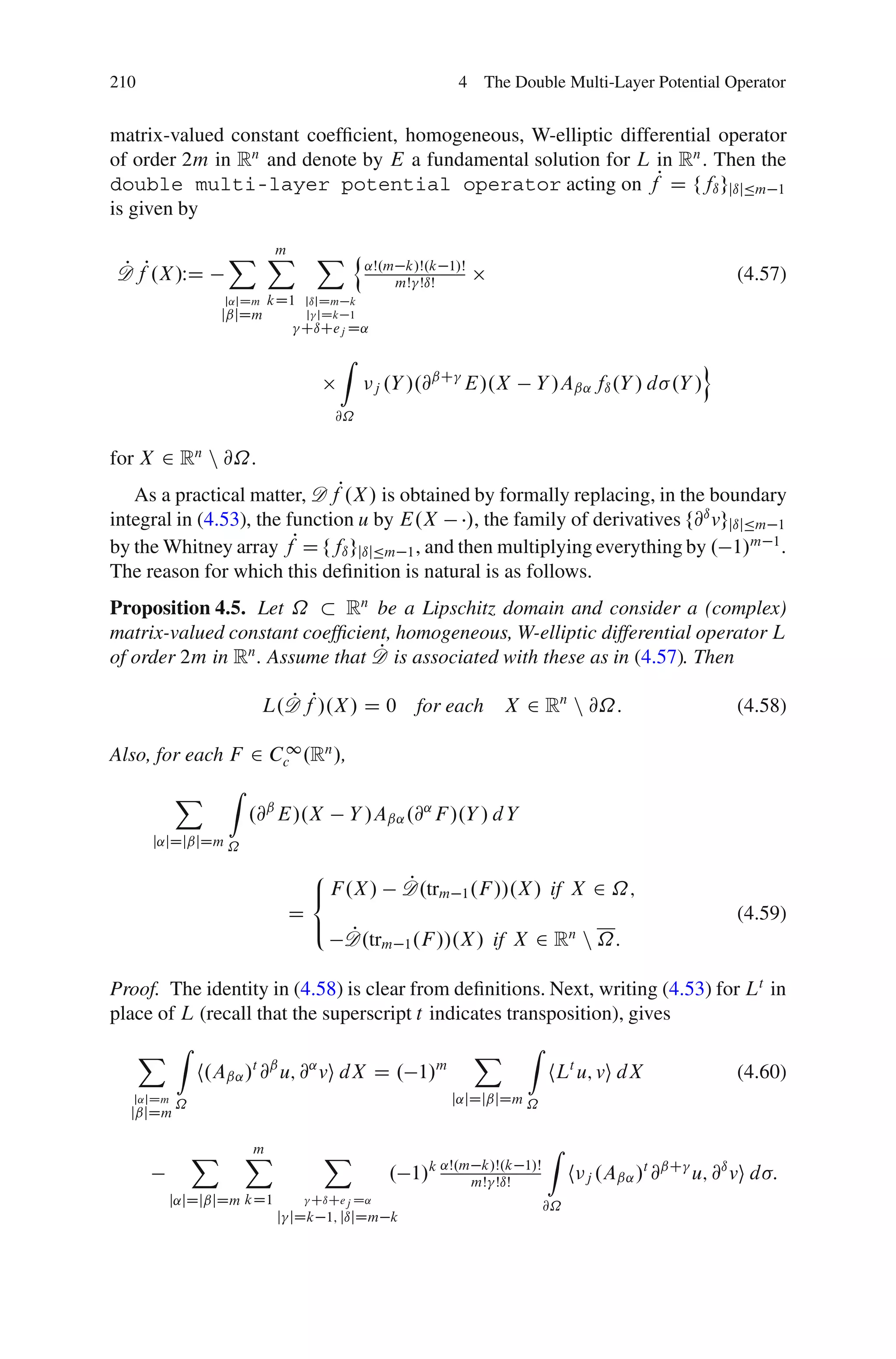
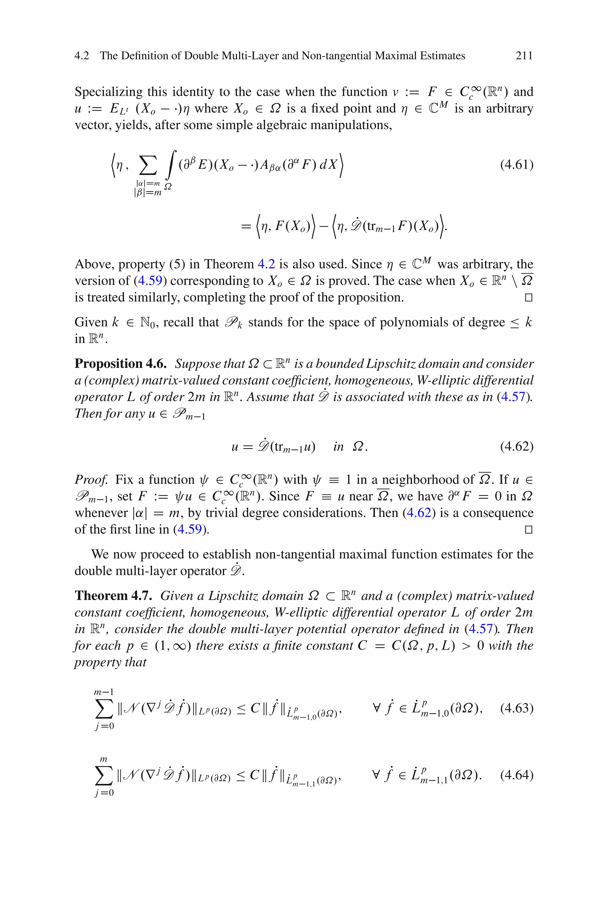
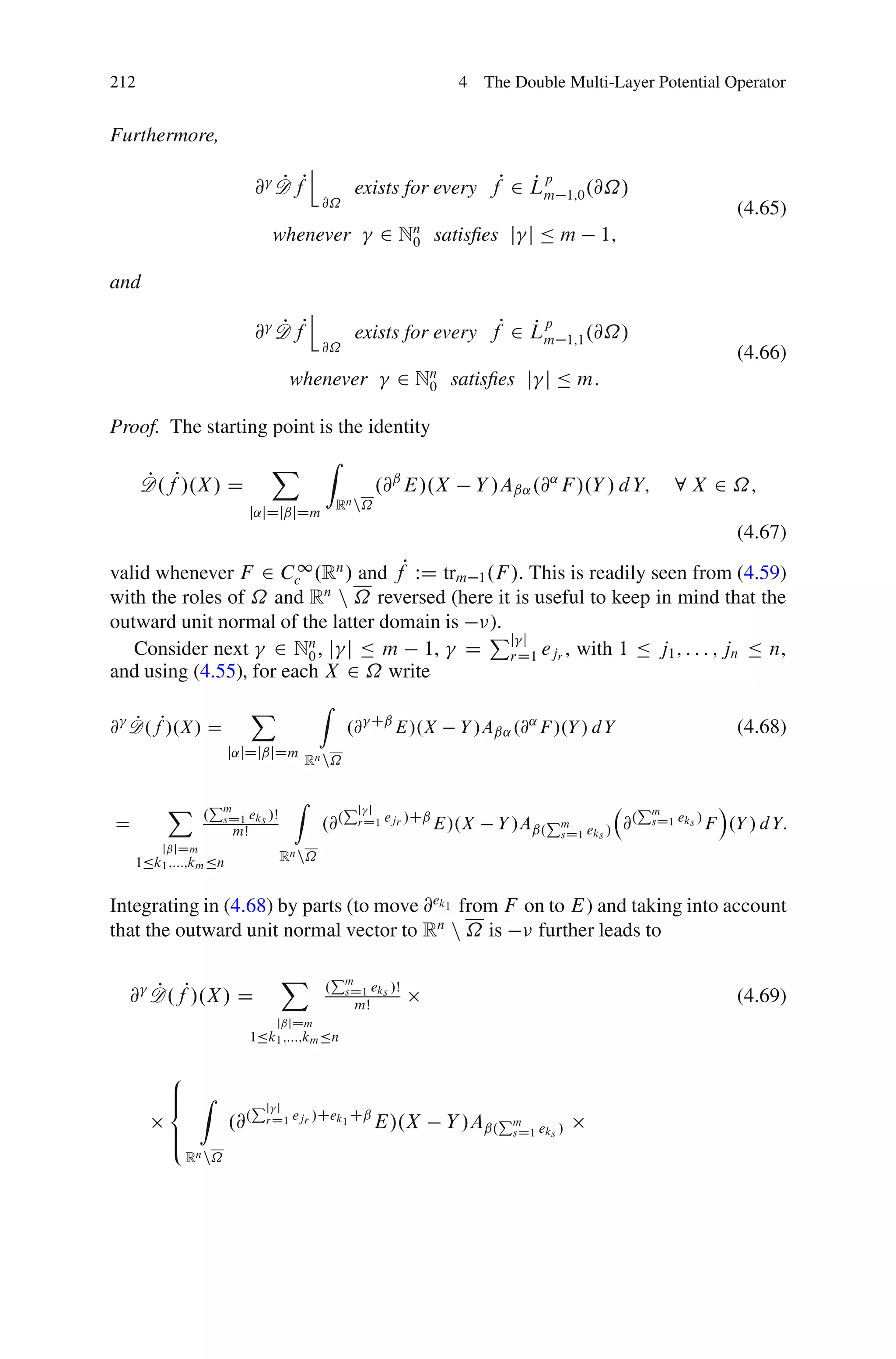
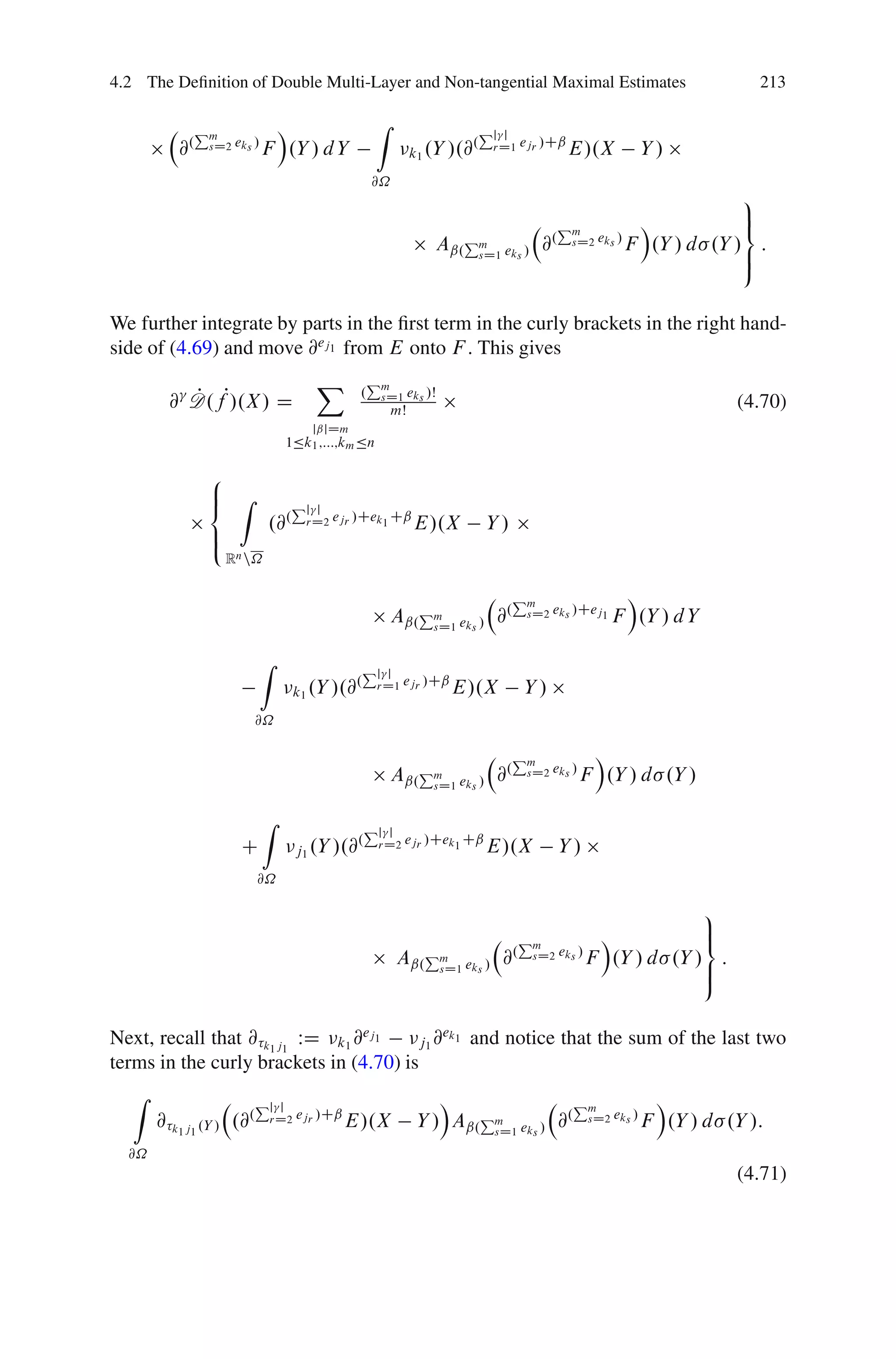
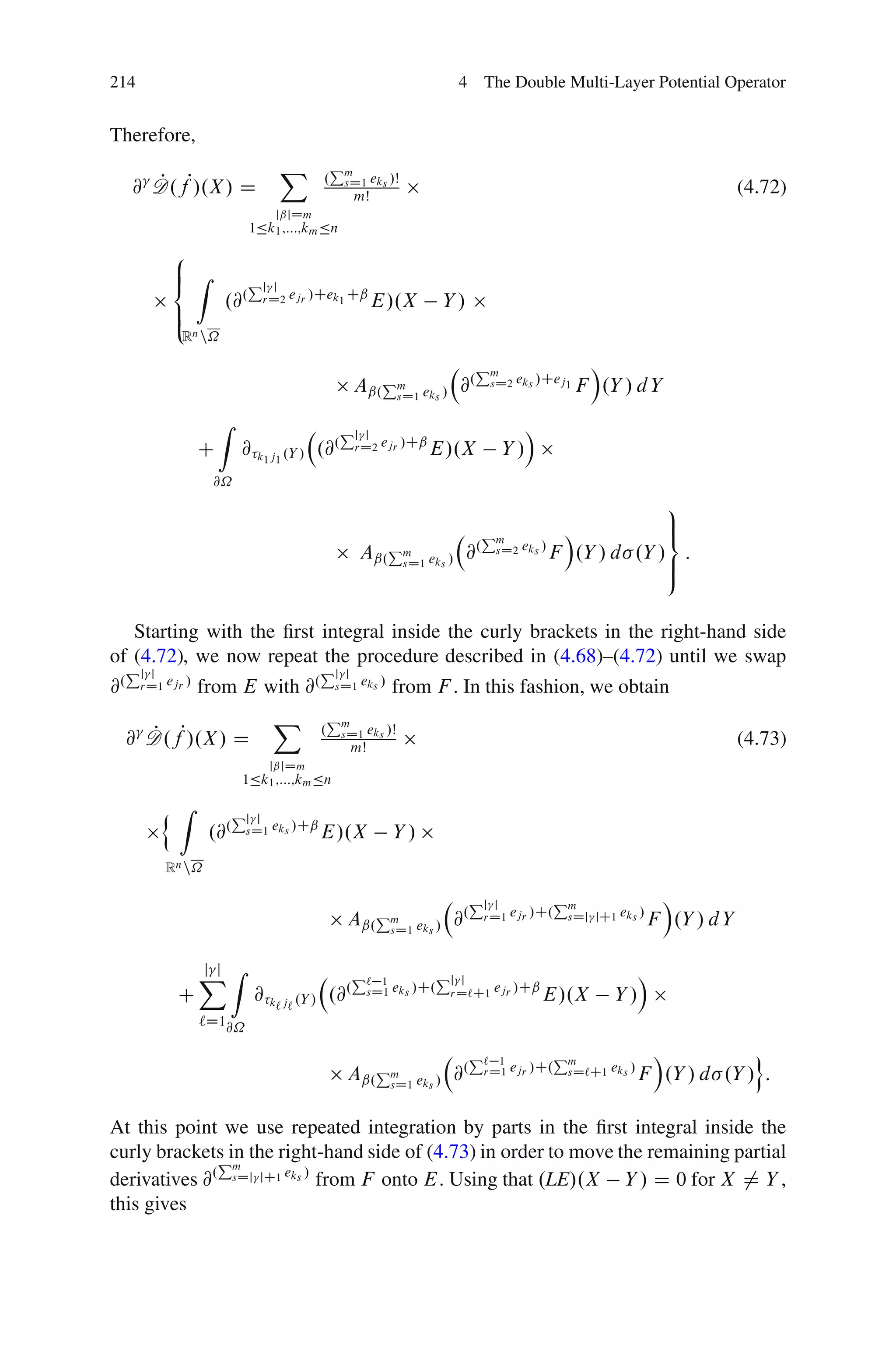
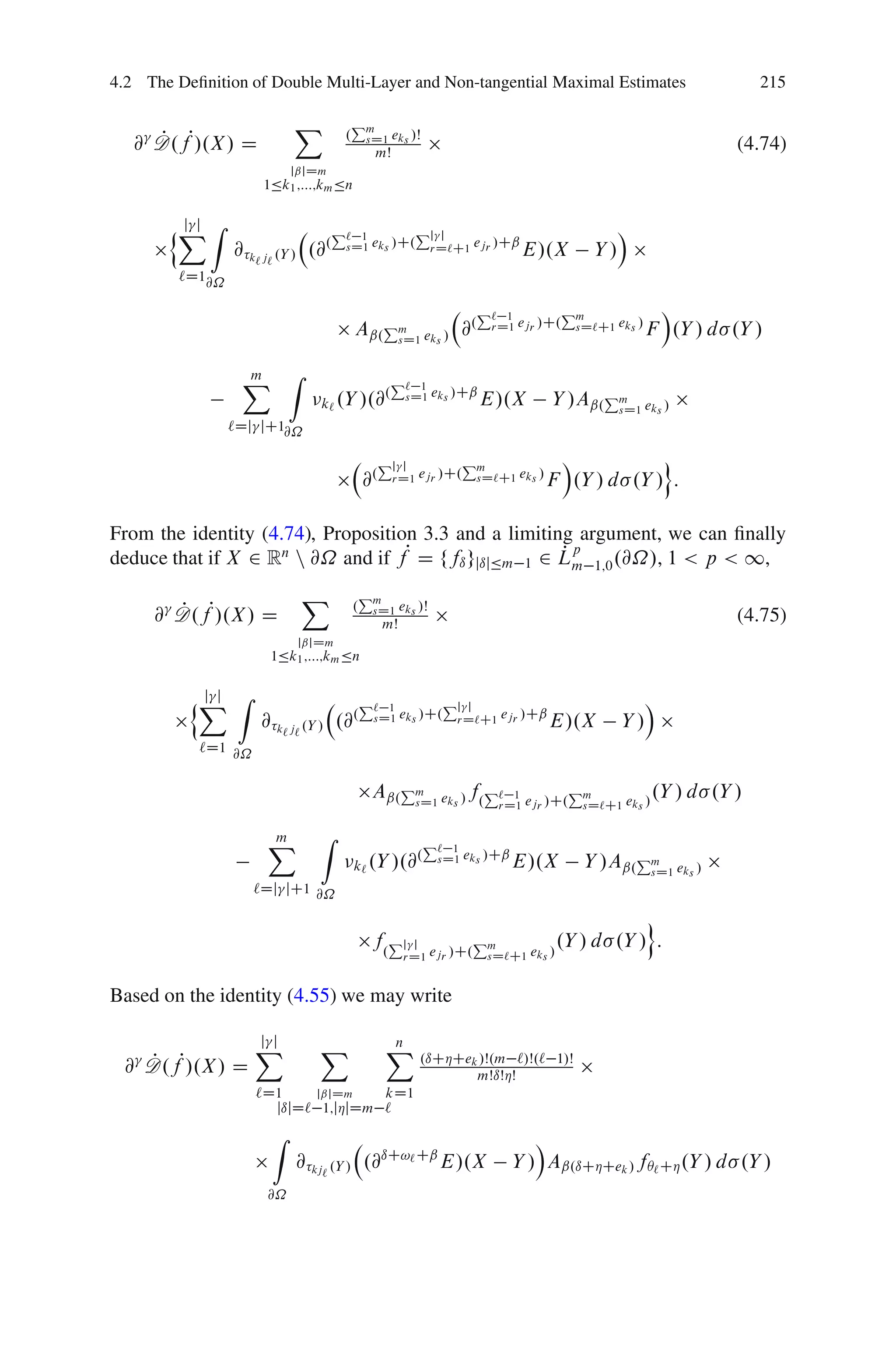
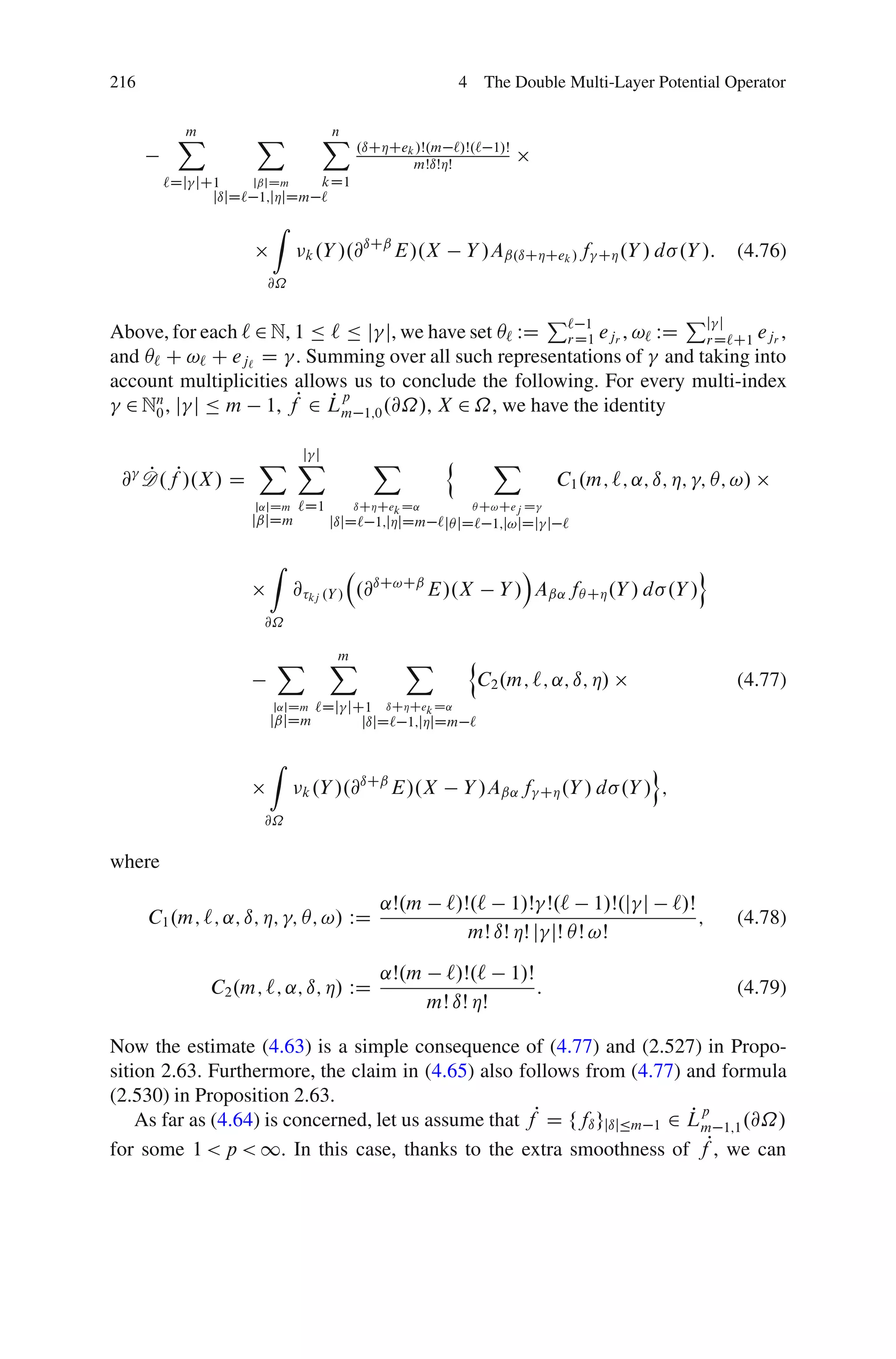
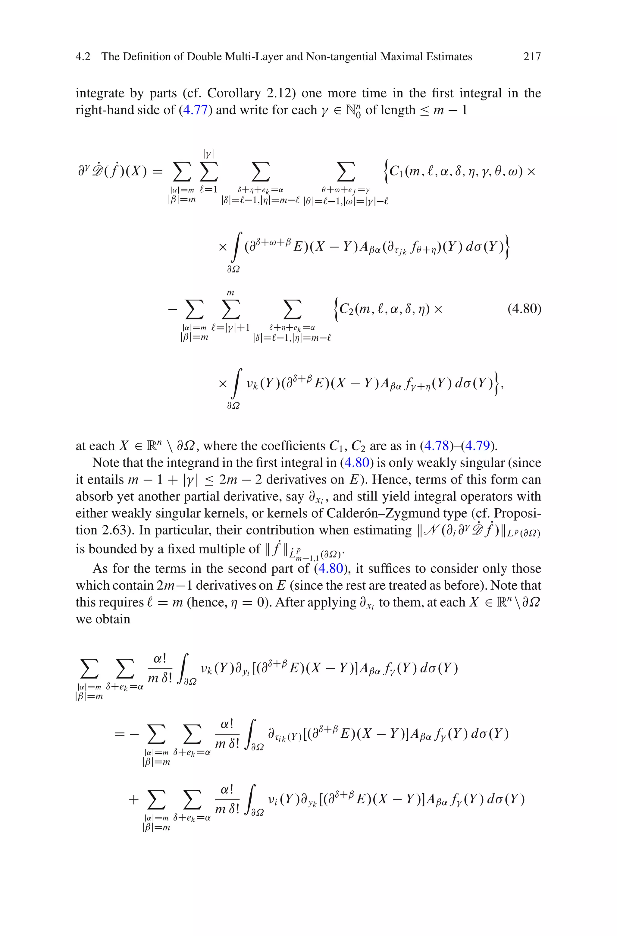
This chapter introduces double multi-layer potential operators associated with elliptic, higher-order, homogeneous, constant coefficient differential operators. It first discusses the nature of fundamental solutions for such operators. It defines various types of ellipticity for a differential operator, including W-ellipticity, ellipticity satisfying the Legendre-Hadamard condition, and S-ellipticity. It also discusses properties like symmetry and self-adjointness of differential operators and their relationship to the coefficients.