Download to read offline
![Mathematica
• Importing data
• Will not read as wide a variety of CSV formats as Gephi
• Can read .gml, .gv, .dot, .graphml, .gxl, .col, .g6, .s6, .gw, .net, .tgf
• Use Map or create a rule to show links (->) from one column of a CSV onto
another
• Other attributes
• More difficult to show vertex/edge attributes than in Gephi but still ppssiblt to
highlight using HighlightGraph[g, x]
• Built-in functions
• Very intuitive and well documented:
https://reference.wolfram.com/language/guide/GraphsAndNetworks.html](https://image.slidesharecdn.com/bookbuyernetwork-160226174025/85/Book-buyer-network-Graph-Analysis-6-320.jpg)
![This graph is
unweighted: edges do not have associated weights
undirected: all edges travel in both directions
contains loops: no vertex is linked directly to itself
simple: undirected, unweighted, loop-free and lacks multiple edges
incomplete: each vertex is not connected to every other vertex
cyclic: contains at least one cycle
not bipartite: vertices cannot be divided into two disjoint sets
UndirectedGraphQ[books]
WeightedGraphQ[books]
CompleteGraphQ[books]
SimpleGraphQ[books]
BipartiteGraphQ[books]
LoopFreeGraphQ[books]
AcyclicGraphQ[books]](https://image.slidesharecdn.com/bookbuyernetwork-160226174025/85/Book-buyer-network-Graph-Analysis-8-320.jpg)
![{6, 4, 4, 23, 8, 7, 11, 8, 25, 16, 15, 18, 25, 13, 9, 5, 3, 5, 3, 5, 10, 5, 7, 9, 9,
5, 9, 9, 3, 4, 20, 11, 5, 9, 5, 10, 5, 7, 7, 8, 18, 8, 6, 5, 5, 6, 4, 18, 4, 8, 3, 6,
5, 5, 6, 4, 4, 5, 13, 5, 6, 4, 6, 4, 9, 7, 21, 6, 4, 5, 7, 15, 22, 21, 16, 16, 13, 7,
5, 8, 4, 4, 9, 8, 23, 5, 14, 5, 5, 6, 5, 8, 3, 7, 7, 4, 6, 6, 5, 12, 12, 5, 4, 2, 3}
VertexDegree[books]
Vertex degrees:
Histogram[VertexDegree[books], ChartStyle -> Blue,
AxesLabel -> {HoldForm[Vertex degree], HoldForm[Frequency]},
PlotLabel -> None, LabelStyle -> {14, GrayLevel[0]}]](https://image.slidesharecdn.com/bookbuyernetwork-160226174025/85/Book-buyer-network-Graph-Analysis-9-320.jpg)
![MatrixForm[GraphDistanceMatrix[books]]
Distance matrix](https://image.slidesharecdn.com/bookbuyernetwork-160226174025/85/Book-buyer-network-Graph-Analysis-10-320.jpg)
![Array plot: distance matrix
ArrayPlot[GraphDistanceMatrix[books]]](https://image.slidesharecdn.com/bookbuyernetwork-160226174025/85/Book-buyer-network-Graph-Analysis-11-320.jpg)
![Max[Flatten[GraphDistanceMatrix[books]]]
OR
GraphDiameter[books]
Diameter = 7
Radius = 4
GraphRadius[books]
Maximum and minimum eccentricities of any vertex:](https://image.slidesharecdn.com/bookbuyernetwork-160226174025/85/Book-buyer-network-Graph-Analysis-12-320.jpg)
![Eccentricity Centrality
HighlightGraph[books, VertexList[books],
VertexSize ->
Thread[VertexList[books] ->
Rescale[EccentricityCentrality[books]]]]
Increases as maximum distances to every other reachable node increases](https://image.slidesharecdn.com/bookbuyernetwork-160226174025/85/Book-buyer-network-Graph-Analysis-13-320.jpg)
![Closeness Centrality
HighlightGraph[books, VertexList[books],
VertexSize ->
Thread[VertexList[books] ->
Rescale[ClosenessCentrality[books]]]]
Increases as average distance to other nodes increases](https://image.slidesharecdn.com/bookbuyernetwork-160226174025/85/Book-buyer-network-Graph-Analysis-14-320.jpg)
![Betweenness Centrality
HighlightGraph[books, VertexList[books],
VertexSize ->
Thread[VertexList[books] ->
Rescale[BetweennessCentrality[books]]]]
Increases as node lies on more shortest paths between other node-pairs](https://image.slidesharecdn.com/bookbuyernetwork-160226174025/85/Book-buyer-network-Graph-Analysis-15-320.jpg)
![Degree Centrality
HighlightGraph[books, VertexList[books],
VertexSize ->
Thread[VertexList[books] ->
Rescale[DegreeCentrality[books]]]]
Increases as vertex degree increases](https://image.slidesharecdn.com/bookbuyernetwork-160226174025/85/Book-buyer-network-Graph-Analysis-16-320.jpg)
![a = ListPlot[EccentricityCentrality[books], Filling -> Axis, PlotStyle -> Red]
b = ListPlot[ClosenessCentrality[books], Filling -> Axis, PlotStyle -> Magenta]
c = ListPlot[RadialityCentrality[books], Filling -> Axis, PlotStyle -> Cyan]
d = ListPlot[DegreeCentrality[books], Filling -> Axis]
gg = GraphicsGrid[{{a, b}, {c, d}}]
Export["CentralityGrid.png", gg]
Eccentricity Closeness
Radiality Degree](https://image.slidesharecdn.com/bookbuyernetwork-160226174025/85/Book-buyer-network-Graph-Analysis-17-320.jpg)
![Dual Hub
HighlightGraph[books, GraphHub[books]]
Nodes with the highest vertex degree are returned](https://image.slidesharecdn.com/bookbuyernetwork-160226174025/85/Book-buyer-network-Graph-Analysis-18-320.jpg)
![Hub Neighbours
HighlightGraph[books, NeighborhoodGraph[books, GraphHub[books]]]](https://image.slidesharecdn.com/bookbuyernetwork-160226174025/85/Book-buyer-network-Graph-Analysis-19-320.jpg)
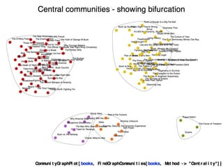
![CommunityGraphPlot[books]
Communities: Small world graph (Modular)](https://image.slidesharecdn.com/bookbuyernetwork-160226174025/85/Book-buyer-network-Graph-Analysis-20-320.jpg)
![Graph partition:
minimises number of endpoints having edges in each part
HighlightGraph[books,FindGraphPartition[books]]](https://image.slidesharecdn.com/bookbuyernetwork-160226174025/85/Book-buyer-network-Graph-Analysis-21-320.jpg)
![Graph communities:
maximises edges joining nodes within communities
with relatively fewer edges joining to nodes in other
communities
HighlightGraph[books, FindGraphCommunities[books]]](https://image.slidesharecdn.com/bookbuyernetwork-160226174025/85/Book-buyer-network-Graph-Analysis-22-320.jpg)
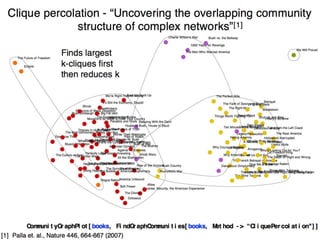
![Cliques
Largest set of connected vertices
HighlightGraph[books, Subgraph[books, FindClique[books]]]](https://image.slidesharecdn.com/bookbuyernetwork-160226174025/85/Book-buyer-network-Graph-Analysis-25-320.jpg)
![Cliques
Largest set of connected vertices within 2 edges of each other
HighlightGraph[books, Subgraph[books, FindKClique[books, 2]]]](https://image.slidesharecdn.com/bookbuyernetwork-160226174025/85/Book-buyer-network-Graph-Analysis-26-320.jpg)
![Cliques
Largest set of connected vertices within 3 edges of each other
HighlightGraph[books, Subgraph[books, FindKClique[books, 3]]]](https://image.slidesharecdn.com/bookbuyernetwork-160226174025/85/Book-buyer-network-Graph-Analysis-27-320.jpg)
![Cliques
Largest set of connected vertices within 4 edges of each other
HighlightGraph[books, Subgraph[books, FindKClique[books, 4]]]](https://image.slidesharecdn.com/bookbuyernetwork-160226174025/85/Book-buyer-network-Graph-Analysis-28-320.jpg)
![Cliques
Largest set of connected vertices within 5 edges of each other
HighlightGraph[books, Subgraph[books, FindKClique[books, 5]]]](https://image.slidesharecdn.com/bookbuyernetwork-160226174025/85/Book-buyer-network-Graph-Analysis-29-320.jpg)
![Cliques
Largest set of connected vertices within 6 edges of each other
HighlightGraph[books, Subgraph[books, FindKClique[books, 6]]]](https://image.slidesharecdn.com/bookbuyernetwork-160226174025/85/Book-buyer-network-Graph-Analysis-30-320.jpg)
![Cliques
Largest set of connected vertices within 7 (=diameter)
edges of each other
HighlightGraph[books, Subgraph[books, FindKClique[books, 7]]]](https://image.slidesharecdn.com/bookbuyernetwork-160226174025/85/Book-buyer-network-Graph-Analysis-31-320.jpg)

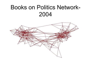
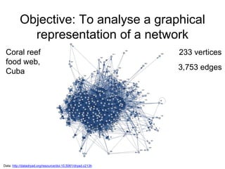
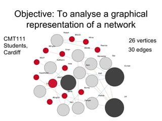
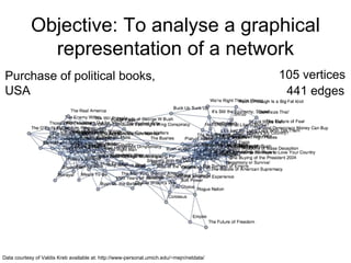
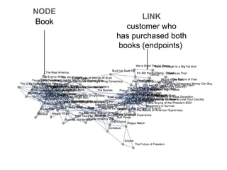
The document analyzes a network graph of purchases of political books in the USA with 105 vertices and 441 edges. It explores various graph metrics and centrality measures including degree, closeness, betweenness, and eccentricity centrality. It identifies graph properties such as the diameter of 7, radius of 4, and presence of communities detected using graph partitioning and community detection algorithms.


