Machine learning lecture pdf

1. Lecture 1.4
• Bias, Variance
• Bias and Variance tradeoff
Dr. Mainak Biswas

2. Bias and Variance
• The total error of a model can be decomposed
into
– Reducible errors (Bias and Variance)
– Irreducible errors (noise)
• The bias-variance trade-off is an important
concept in statistics and machine learning
Dr. Mainak Biswas

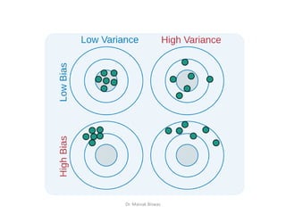
3. Bias
• The inability of a model to accurately capture
the true relationship is called bias
• Models with high bias are simple and fail to
capture the complexity of the data
• Low bias corresponds to a good fit to the
training dataset
Dr. Mainak Biswas

4. Variance
• Variance refers to the amount by which the
estimate of the true relationship would
change on using a different training dataset
• High variance implies that the model does not
perform well on previously unseen data
(testing data) even if it fits the training data
well
• Low variance implies that the model performs
well on the testing set
Dr. Mainak Biswas

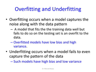
5. Overfitting and Underfitting
• Overfitting occurs when a model captures the
noise along with the data pattern
– A model that fits the the training data well but
fails to do so on the testing set is an overfit to the
data.
– Overfitted models have low bias and high
variance.
• Underfitting occurs when a model fails to even
capture the pattern of the data
– Such models have high bias and low variance
Dr. Mainak Biswas

6. Dr. Mainak Biswas

7. The Bias-Variance Trade-off
• This is a way to make sure that the model is
neither overfitted nor underfitted
• Ideally, a model should have low bias so that it
can accurately model the true relationship and
low variance so that it can produce consistent
results and perform well on testing data
• This is called a trade-off as it is challenging to
find a model for which both the bias and
variance are low
Dr. Mainak Biswas

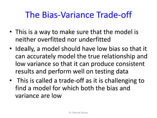
8. Total Error
OR
• This equation suggests that we need to find a model that
simultaneously achieves low bias and low variance
• Variance is a non-negative term and bias squared is also non
negative which implies the total error can never go below the
irreducible error
Dr. Mainak Biswas

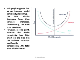
9. • This graph suggests that
as we increase model
complexity(flexibility),
the bias initially
decreases faster than
variance increases,
consequently, the total
error decreases
• However, at one point,
increase the model
complexity has little
effect on the bias but
the variance increases
significantly,
consequently , the total
error also increases
Dr. Mainak Biswas

10. Derivation of Total Error 1
• We have independent variables x that affect the value of a
dependent variable y
• Function f denotes the true relationship between x and y
• In real life problems it is very hard to know this relationship
• y is given by this formula along with some noise which is
represented by the random variable ϵ with zero mean and
variance σϵ²
Where,
Dr. Mainak Biswas

11. Derivation of Total Error 2
• Now, when we try to model the underlying real-life problem, we try to find a
function 𝒇 that can accurately predict the true relationship 𝒇
• The goal is to bring the prediction as close as possible to the actual value
(𝑦 ≈ 𝑓(𝑥)) to minimize the error
• 𝔼[(𝑦 − 𝑓(𝑥))²] is called Mean Squared Error, commonly known as MSE
• This is defined as the average squared difference of a prediction f̂(x) from its true
value y.
• Bias is defined as the difference of the average value of prediction from the true
relationship function f(x)
• Variance is defined as the expectation of the squared deviation of f̂(x) from its
expected value 𝔼[f̂(x)]
Dr. Mainak Biswas

12. Derivation of Total Error 3
Dr. Mainak Biswas

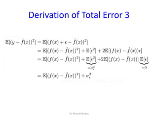
13. Derivation of Total Error 4
• Now, by further expanding the term on the
RHS, 𝔼*(f(x) −f̂(x))²]
Dr. Mainak Biswas

14. Derivation of Total Error 5
• 𝔼[f̂(x)] − f(x) is a constant since we subtract f(x), a
constant , from 𝔼[f̂(x)] which is also a constant
• So, 𝔼[(𝔼[f̂(x)] − f(x))²] = (𝔼[f̂(x)] − f(x))²
• Further expanding using the linearity property of
expectation we get the value of 𝔼[(f(x) −f̂(x))²]
• Plugging this value back into the equation for
𝔼[(y −f̂(x))²], we arrive on our final equation
Dr. Mainak Biswas