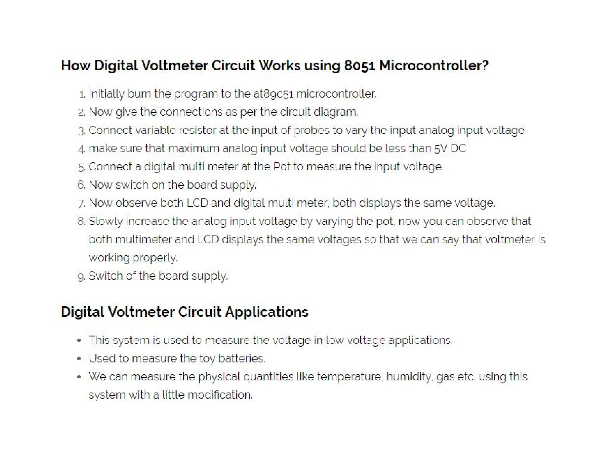
The technology ofVirtual Instruments (cont.)
• Advantages of Virtual Instruments versus Traditional
Instruments
Flexibility
You can easily add additional functions such as a filter routine
or a new data view to a virtual instrument.
Storage
Today's personal computers have hard disks that can store
dozens of gigabytes which is an absolute plus if you want to
process mass data like audio or video.
Display
Computer monitors usually have better color depth and pixel
resolution than traditional instruments. Also you can switch
easily between different views of the data (graphical,
numerical).
4.
What is VirtualInstrumentation?
Virtual instrumentation combines mainstream commercial technologies.
such as C, with flexible software and a wide variety of measurement
and control hardware, so engineers and scientists can create user-
defined systems that meet their exact application needs. With virtual
instrumentation, engineers and scientists reduce development time,
design higher quality products, and lower their design costs.
5.
Why is VirtualInstrumentation necessary?
Virtual instrumentation is necessary because it delivers
instrumentation with the rapid adaptability required for today’s
concept, product, and process design, development, and
delivery. Only with virtual instrumentation can engineers and
scientists create the user-defined instruments required to keep
up with the world’s demands.
The only way to meet these demands is to use test and control
architectures that are also software centric. Because virtual
instrumentation uses highly productive software, modular I/O,
and commercial platforms, it is uniquely positioned to keep
pace with the required new idea and product development rate
6.
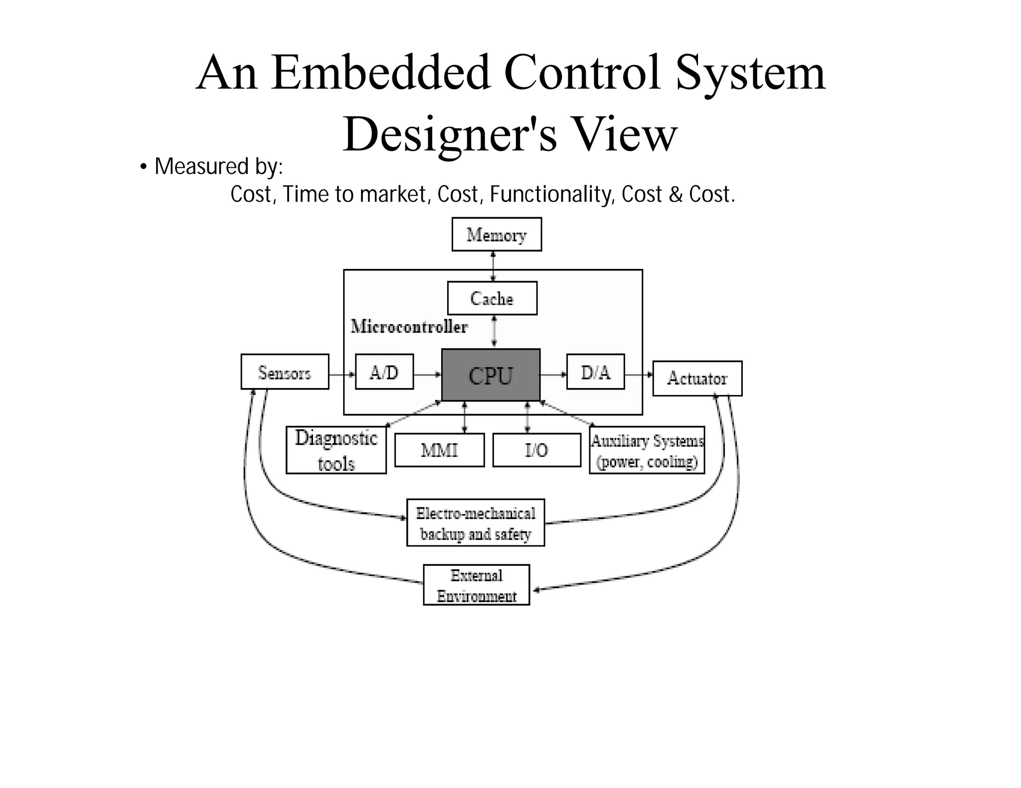
The technology ofVirtual Instruments
Virtual Instrumentation is the use of customizable software and
modular measurement hardware to create user-defined measurement
systems, called virtual instruments.
Computer
Software
Hardware
7.
What is avirtual instrument and how is it different
from a traditional instrument?
Every virtual instrument consists of two parts – software and
hardware. A virtual instrument typically has a sticker price
comparable to and many times less than a similar traditional
instrument for the current measurement task.
A traditional instrument provides them with all software and
measurement circuitry packaged into a product with a finite list of
fixed-functionality using the instrument front panel. A virtual
instrument provides all the software and hardware needed to
accomplish the measurement or control task. In addition, with a
virtual instrument, engineers and scientists can customize the
acquisition, analysis, storage, sharing, and presentation functionality
using productive, powerful software.
8.
Traditional instruments (left)and software based virtual instruments (right) largely
share the same architectural components, but radically different philosophies
9.
One Application --Different Devices
For this particular example, an engineer is developing an
application using LabVIEW and an M Series DAQ board on a
desktop computer PCI bus in his lab to create a DC voltage and
temperature measurement application. After completing the
system, he needs to deploy the application to a PXI system on the
manufacturing floor to perform the test on new product.
Alternatively, he may need the application to be portable, and so
he selects NI USB DAQ products for the task. In this example,
regardless of the choice, he can use virtual instrumentation in a
single program in all three cases with no code change needed.
10.
Virtual Instrumentation forIndustrial I/O and
Control
• PCs and PLCs both play an important role in control and
industrial applications. PCs bring greater software flexibility
and capability, while PLCs deliver outstanding ruggedness and
reliability. But as control needs become more complex, there is
a recognized need to accelerate the capabilities while retaining
the ruggedness and reliabilities.
• Multi domain functionality (logic, motion, drives, and process)
– the concept supports multiple I/O types. Logic, motion, and
other function integration is a requirement for increasingly
complex control approaches.
• Software tools for designing applications across several
machines or process units – the software tools must scale to
distributed operation.
11.
Virtual Instrumentation forDesign
• The same design engineers that use a wide variety of software
design tools must use hardware to test prototypes. Commonly,
there is no good interface between the design phase and
testing/validation phase, which means that the design usually
must go through a completion phase and enter a
testing/validation phase. Issues discovered in the testing phase
require a design-phase reiteration.
12.
On which hardwareI/O and platforms does virtual
instrumentation software run?
• Standard hardware platforms that house the I/O are important to I/O
modularity. Laptop and desktop computers provide an excellent
platform where virtual instrumentation can make the most of existing
standards such as the USB, PCI, Ethernet, and PCMCIA buses.
• for example, USB 2.0 and PCI Express
13.
Layers of VirtualInstrumentation
• Application Software: Most people think immediately of the
application software layer. This is the primary development
environment for building an application.
• Test and Data Management Software: Above the application
software layer the test executive and data management
software layer. This layer of software incorporates all of the
functionality developed by the application layer and provides
system-wide data management.
• Measurement and Control Services Software: The last layer is
often overlooked, yet critical to maintaining software
development productivity.
14.
Advantages of VirtualInstruments versus
Traditional Instruments
Flexibility
You can easily add additional functions such as a filter routine
or a new data view to a virtual instrument.
Storage
Today's personal computers have hard disks that can store
dozens of gigabytes which is an absolute plus if you want to
process mass data like audio or video.
Display
Computer monitors usually have better color depth and pixel
resolution than traditional instruments. Also you can switch
easily between different views of the data (graphical,
numerical).
Costs
PC add-in boards for signal acquisition and software mostly
cost a fraction of the traditional hardware they emulate.
15.
• Block diagramexecutes
dependent on the flow of data;
block diagram does NOT
execute left to right
• Node executes when data is
available to ALL input
terminals
• Nodes supply data to all output
terminals when done
Dataflow Programming
16.
Help Options
Context Help
•Online help
• Lock help
• Simple/Complex Diagram help
• Ctrl + H
Online reference
• All menus online
• Pop up on functions in diagram to access online info
directly
17.
Graphical programming indata
flow
LabVIEW
LabVIEW is a graphical programming language that uses icons
instead of lines of text to create applications. In contrast to text-
based programming languages, where instructions determine
program execution, LabVIEW uses dataflow programming, where
the flow of data determines execution order.
You can purchase several add-on software toolkits for developing
specialized applications. All the toolkits integrate seamlessly in
LabVIEW. Refer to the National Instruments Web site for more
information about these toolkits.
LabVIEW also includes several wizards to help you quickly
configure your DAQ devices and computer-based instruments and
build applications
18.
LabVIEW programs arecalled virtual instruments (VIs).
Controls are inputs and indicators are outputs.
Each VI contains three main parts:
•Front Panel – How the user interacts with the VI.
•Block Diagram – The code that controls the program.
•Icon/Connector – Means of connecting a VI to other VIs.
In LabVIEW, you build a user interface by using a set of tools and
objects. The user interface is known as the front panel. You then
add code using graphical representations of functions to control
the front panel objects. The block diagram contains this code. In
some ways, the block diagram resembles a flowchart
19.
Users interact withthe Front Panel when the program is
running. Users can control the program, change inputs, and
see data updated in real time. Controls are used for inputs
such as, adjusting a slide control to set an alarm value,
turning a switch on or off, or to stop a program. Indicators
are used as outputs. Thermometers, lights, and other
indicators display output values from the program. These
may include data, program states, and other information.
Every front panel control or indicator has a corresponding
terminal on the block diagram. When a VI is run, values
from controls flow through the block diagram, where they
are used in the functions on the diagram, and the results are
passed into other functions or indicators through wires.
Front Panel
Controls =Inputs
Indicators = Outputs
Block Diagram
Accompanying “program” for
front panel
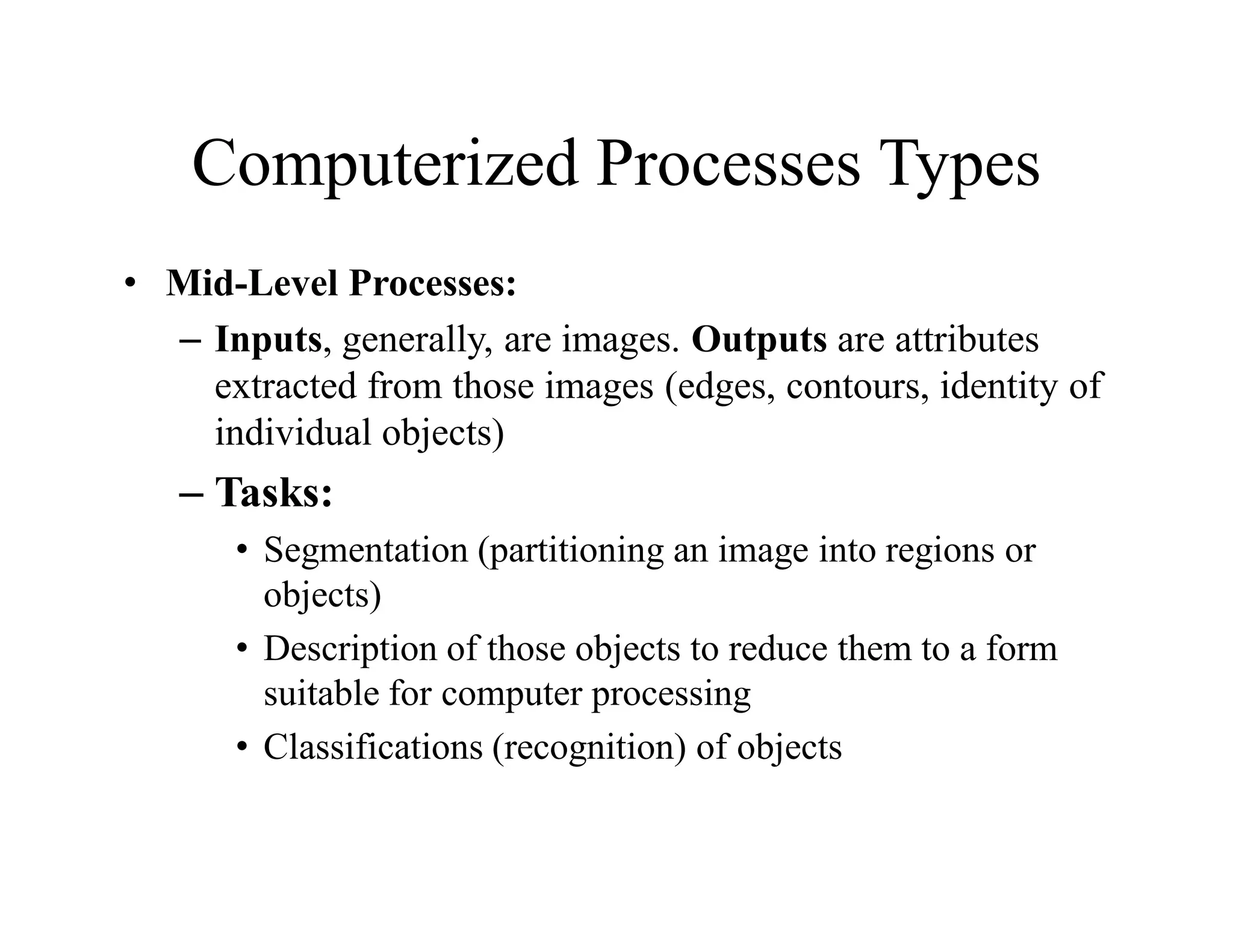
Components “wired” together
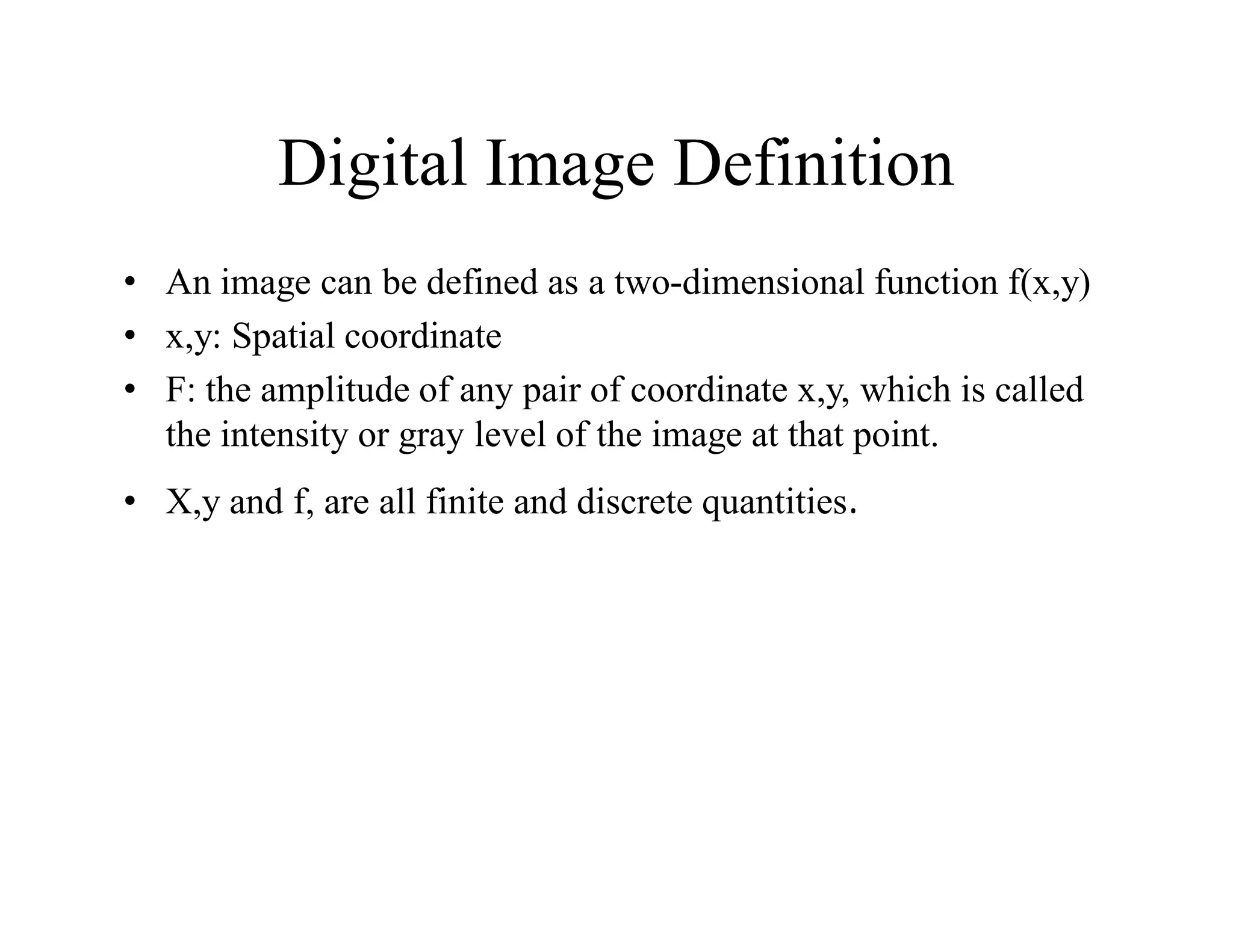
LabVIEW Programs Are Called Virtual
Instruments (VIs)
VI Block Diagram
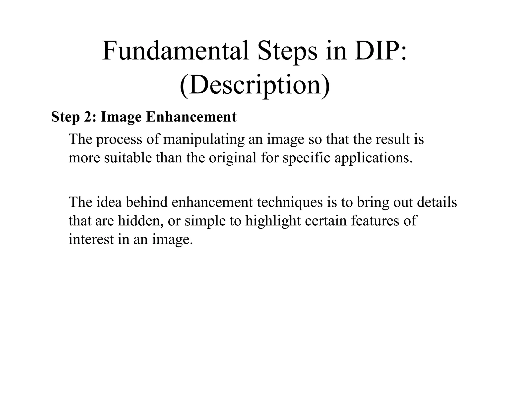
NumericConstant
Thermometer
Terminal
Call to
subVI
While Loop
Knob
Terminal
Stop Button
Terminal
Stop Loop
Terminal
Temperature
Graph
24.
Controls and FunctionsPalettes
Graphical, floating palettes
Used to place controls &
indicators on the front panel, or
to build the block diagram
Controls Palette
(Panel Window)
Functions Palette
(Diagram Window)
25.
Operating Tool
Positioning/Resizing Tool
LabelingTool
Wiring Tool
Shortcut Menu Tool
• Floating Palette
• Used to operate and modify front
panel and block diagram objects.
Scrolling Tool
Breakpoint Tool
Probe Tool
Color Copy Tool
Coloring Tool
Tools Palette
Automatic Selection Tool
26.
Run Button
Continuous Run
Button
AbortExecution
Pause/Continue
Button
Text Settings
Align Objects
Distribute Objects
Reorder
Execution
Highlighting Button
Step Into Button
Step Over Button
Step Out Button
Additional Buttons on
the Diagram Toolbar
Status Toolbar
27.
Signal Generation
and Processing.vi
Help» Find Examples…
Browse According to: Task
» Analyzing and Processing Signals
» Signal Processing
» Signal Generation and Processing.vi
Open and Run a Virtual Instrument
Creating a VI– Block Diagram
• After Creating Front Panel Controls and Indicators, Switch to
Block Diagram <Ctrl-E>
• Move Front Panel Objects to Desired Locations Using the
Position/Size/Select Tool
• Place Functions On Diagram
• Wire Appropriate Terminals Together to Complete the
Diagram
30.
Wiring Tips –Block Diagram
Wiring “Hot Spot”
Click While Wiring To Tack Wires Down
Spacebar Flips Wire Orientation
Click To Select Wires
SubVIs
• A SubVIis a VI that can be used within
another VI
• Advantages
– Modular
– Easier to debug
– Don’t have to recreate code
– Require less memory
33.
Icon and Connector
•An icon represents a VI in other block
diagrams
• A connector shows available terminals
for data transfer
Icon
Connector
Terminals
Save The VI
•Choose an Easy to Remember Location
• Organize by Functionality
– Save Similar VIs into one directory (e.g. Math Utilities)
• Organize by Application
– Save all VIs Used for a Specific Application into one
directory or library file (e.g. Lab 1 – Frequency Response)
• Library Files (.llbs) combine many VI’s into a single
file, ideal for transferring entire applications across
computers
40.
Insert the SubVIinto a Top Level VI
Accessing user-made subVIs
Functions >> Select a VI
Or
Drag icon onto target diagram
41.
Tips for Workingin LabVIEW
• Keystroke Shortcuts
– <Ctrl-H> – Activate/Deactivate Context Help Window
– <Ctrl-B> – Remove Broken Wires From Block Diagram
– <Ctrl-E> – Toggle Between Front Panel and Block
Diagram
– <Ctrl-Z> – Undo (Also in Edit Menu)
• Tab Key – Toggle Through Tools on Toolbar
• Tools » Options… – Set Preferences in LabVIEW
• VI Properties – Configure VI Appearance,
Documentation, etc.
Loops
• While Loops
–Have Iteration Terminal
– Always Run Once
– Run According to
Continue Terminal
• For Loops
– Have Iteration Terminal
– Run According to input N
File I/O
•Read/write to
spreadsheetfile
•Read/write characters to
file (ASCII)
•Read lines from file
•Read/write binary file
Easy File I/O
Easy File I/O
VIs
VIs
54.
Array Functions &Graphs
• Basic Array Functions
• Use graphs
• Create multiplots with graphs
Graphs
• Selected fromthe Graph palette of Controls menu
–Waveform Graph – Plot an
array of numbers against
their indices
–XY Graph – Plot one array
against another
–Digital Waveform Graph –
Plot bits from binary data
58.
Strings
• A stringis a sequence of displayable or nondisplayable
characters (ASCII)
• Many uses – displaying messages, instrument control, file I/O
• String control/indicator is in the Controls»String subpalette
59.
Clusters
• Data structurethat groups data together
• Data may be of different types
• Analogous to struct in C
• Elements must be either all controls or all indicators
• Thought of as wires bundled into a cable
60.
Creating a Cluster
1.Select a Cluster shell
from the Array &
Cluster subpalette
2. Place objects inside the
shell
61.
Cluster Functions
• Inthe Cluster subpalette of the Functions palette
• Can also be accessed by right-clicking on the cluster
terminal
Bundle
(Terminal labels
reflect data type)
Bundle By Name
Error Clusters
• Errorcluster contains the following information:
– Boolean to report whether error occurred
– Integer to report a specific error code
– String to give information about the error
64.
Error Handling Techniques
•Error information is passed from one subVI to the next
• If an error occurs in one subVI, all subsequent subVIs are not
executed in the usual manner
• Error Clusters contain all error conditions
error clusters
65.
Case Structures
• Inthe Structures sub palette of Functions palette
• Enclose nodes or drag them inside the structure
• Stacked like a deck of cards, only one case visible
Sequence Structures
• Inthe Structures subpalette of Functions palette
• Executes diagrams sequentially, Frame 0 (0..x), where x is the
total number of frames
• Stacked like a deck of cards, only one frame visible
68.
Sequence Locals
• Passdata from one frame to future frames
• Created at the border of the Sequence structure
Sequence local
created in
Frame 1
Data not
available
Data
available
69.
Formula Nodes
• Inthe Structures subpalette
• Implement complicated equations
• Variables created at border
• Variable names are case sensitive
• Each statement must terminate with a semicolon (;)
• Context Help Window shows available functions
Note semicolon
70.
Printing & Documentation
•Print From File Menu to Printer, HTML, Rich Text File
• Programmatically Print Graphs or Front Panel Images
• Document VIs in VI Properties » Documentation Dialog
• Add Comments Using Free Labels on Front Panel & Block
Diagram
71.
Printing
• File »Print… Gives Many Printing Options
– Choose to Print Icon, Front Panel, Block Diagram, VI
Hierarchy, Included SubVIs, VI History
• Print Panel.vi (Functions » Application Control)
Programmatically Prints a Front Panel
• Generate & Print Reports (Functions » Report Generation)
– Search in Find Examples for Report Generation
72.
Documenting VIs
• VIProperties » Documentation
– Provide a Description and Help Information for a VI
• VI Properties » Revision History
– Track Changes Between Versions of a VI
• Individual Controls » Description and Tip…
– Right Click to Provide Description and Tip Strip
• Use Labeling Tool to Document Front Panels & Block Diagrams
73.
Simple VI Architecture
•Functional VI that produces results when run
– No “start” or “stop” options
– Suitable for lab tests, calculations
• Example: Convert C to F.vi
State Machine Architecture
•Advantages
– Can go from any state from any
other
– Easy to modify and debug
• Disadvantages
– Can lose events if two occur at the
same time
States:
0: Startup
1: Idle
2: Event 1
3: Event 2
4:Shutdown
Introduction to DAQ
•Data Acquisition – “Sampling of the real world to generate
data that can be analyzed and presented by a computer.”
79.
PC Based DataAcquisition System Overview:
In the last few years, industrial PC I/O interface products have
become increasingly reliable, ccurate and affordable. PC-based data
acquisition and control systems are widely used in industrial and
laboratory applications like monitoring, control, data acquisition and
automated testing.
Selecting and building a DA&C (Data Acquisition and Control)
system that actually does what you want it to do requires some
knowledge of electrical and computer engineering.
• Transducers and actuators
• Signal conditioning
• Data acquisition and control hardware
• Computer systems software
80.
Data acquisition SystemIntroduction I:
Data acquisition involves gathering signals from measurement
sources and digitizing the signals for storage, analysis, and
presentation on a PC. Data acquisition systems come in many
different PC technology forms to offer flexibility when choosing
your system. You can choose from PCI, PXI, PCI Express, PXI
Express, PCMCIA, USB, wireless, and Ethernet data acquisition for
test, measurement, and automation applications.
81.
Data acquisition SystemIntroduction II:
All industrial processing systems, factories, machinery, test facilities,
and vehicles consist of hardware components and computer software
whose behavior follow the laws of physics as we understand them.
These systems contain thousands of mechanical and electrical
phenomena that are continuously changing; they are not steady state.
The measurable quantities that represent the characteristics of all
systems are called variables. The proper functioning of a particular
system depends on certain events in time and the parameters of these
variables.
Often, we are interested in the location, magnitude, and speed of the
variables, and we use instruments to measure them.
We assign the variables units of measure such as volts, pounds, and
miles per hour, to name a few.
83.
Transducers:
Data acquisition systemshave multiple components that work together to
gather and process information. They can be used to analyze information
regarding physical phenomena, such as temperature, voltage, and pressure.
However, because temperature, voltage, and pressure are all distinct
different, they require different systems of measurement and
representation. In data acquisition systems, a transducer serves as the
component that translates raw data into a comprehensible electrical signal.
When a data acquisition system uses DAQ (data acquisition hardware) the
transducer also functions as a sensor, gathering the data from which it will
then generate a signal. As a result of all the different variables data
acquisition systems can measure, there are several kinds of transducers. A
transducer must be capable of generating different signals depending on the
particular phenomenon measured. Two general types of signals commonly
are used: analog and digital.
84.
Transducer and Acutuator:
Atransducer converts temperature, pressure, level, length, position,
etc. into voltage, current, frequency, pulses or other signals.
An actuator is a device that activates process control equipment by
using pneumatic, hydraulic or electrical power. For example, a valve
actuator opens and closes a valve to control fluid rate.
85.
Signal conditioning :
Signalconditioning circuits improve the quality of signals generated
by transducers before they are converted into digital signals by the
PC's data-acquisition hardware.
Examples of signal conditioning are signal scaling, amplification,
linearization, cold-junction compensation, filtering, attenuation,
excitation, common-mode rejection, and so on.
86.
One of themost common signal conditioning functions is
amplification. For maximum resolution the voltage range of the
input signals should be approximately equal to the maximum
input range of the A/D converter.
Amplification expands the range of the transducer signals so that
they match the input range of the A/D converter. For example, a x
10 amplifier maps transducer signals which range from 0 to 1 V
onto the range 0 to 10 V before they go into the A/D converter.
87.
Signal Conditioning
Amplification
Isolation
Filtering
Linearization
Electrical signals are conditioned so they can be used by an analog
input board.
The following features may be available:
88.
Data acquisition
Data acquisitionand control hardware generally performs one or
more of the following functions:
•analog input,
•analog output,
•digital input,
•digital output and
•counter/timer functions.
89.
Analog input
An analoginput converts a voltage level into a digital value that can
be stored and processed in a computer. Why would you want to
measure voltages? There are a multitude of sensors available which
convert things like temperature, pressure, etc. into voltages. The
voltages can then be easily measured by various kinds of hardware,
such as a LabJack U3-HV, and then read into a computer. The
computer can then convert the voltage value into it's original type
(temperature, pressure, etc) and the value can then be stored in a file,
emailed to someone, or used to control something else outside of the
computer.
90.
The most significantcriteria when selecting A/D hardware are:
1. Number of input channels
2. Single-ended or differential input signals
3. Sampling rate (in samples per second)
4. Resolution (usually measured in bits of resolution)
5. Input range (specified in full-scale volts)
6. Noise and nonlinearity
91.
Analog to DigitalConverter
An Analog to Digital Converter (ADC) is a very useful
feature that converts an analog voltage on a pin to a
digital number. By converting from the analog world to
the digital world, we can begin to use electronics to
interface to the analog world around us.
Not every pin on a microcontroller has the ability to do analog to
digital conversions. On the Arduino board, these pins have an ‘A’
in front of their label (A0 through A5) to indicate these pins can
read analog voltages.
ADCs can vary greatly between microcontroller. The ADC on the
Arduino is a 10-bit ADC meaning it has the ability to detect 1,024
(210) discrete analog levels.
Some microcontrollers have 8-bit ADCs (28 = 256 discrete levels)
and some have 16-bit ADCs (216 = 65,535 discrete levels).
92.
Analog
Input
4 Samples/cycle
8 Samples/cycle
16Samples/cycle
Sampling rate
Sampling rate is the speed at which the
digitizer’s ADC converts the input signal,
after the signal has passed through the analog
input path, to digital values. Hence, the
digitizer samples the signal after any
attenuation, gain, and/or filtering has been
applied by the analog input path, and converts
the resulting waveform to digital
representation. The sampling rate of a high-
speed digitizer is based on the sample clock
that controls when the ADC converts the
instantaneous analog voltage to digital values
93.
Effective rate ofeach individual channel is inversely proportional to the number
of channels sampled.
Example:
100 KHz maximum.
16 channels.
100 KHz/16 = 6.25 KHz per channel.
94.
A/D converter Range
Dynamicrange is often a key parameter within signal processing
systems and a shortfall can limit the quality and range of signals that
can be received. The technical progress made on improving this
gateway between the analogue and digital world has not kept pace
with Moore's law because the challenges are more fundamental than
simply reducing transistor sizes. Methods to increase a/d converter
dynamic range are therefore always of interest, although each
solution often suits particular applications.
96.
Analog output (D/A)
Ananalog output is a measurable electrical signal with a defined
range that is generated by a controller and sent to a controlled
device, such as a variable speed drive or actuator.
Changes in the analog output cause changes in the controlled device
that result in changes in the controlled process.
Controller output digital to analog circuitry is typically limited to a
single range of voltage or current, such that output transducers are
required to provide an output signal that is compatible with
controlled devices using something other than the controller's
standard signal.
Common Types:There are four common types of analog outputs;
voltage, current, resistance and pneumatic.
• It canbe the most critical factor in obtaining reliable, high
performance operation.
• Transforms the PC and DAQ hardware into a complete DAQ,
analysis, and display system.
• Different alternatives:
– Programmable software.
– Data acquisition software packages.
Data Aquisition software
99.
Programmable software
• Involvesthe use of a programming language, such as:
– C++, visual C++
– BASIC, Visual Basic + Add-on tools (such as
VisuaLab with VTX)
– Fortran
– Pascal
Advantage: flexibility
Disadvantages: complexity and steep learning curve
100.
Data acquisition software
•Does not require programming.
• Enables developers to design the custom instrument
best suited to their application.
Examples: TestPoint, SnapMaster, LabView,
DADISP, DASYLAB, etc.
Below is an image with LabView:
101.
Small Computer SystemInterface [SCSI]
Small Computer System Interface (SCSI), an ANSI
standard, is a parallel interface standard used by Apple
Macintosh computers, PCs, and many UNIX systems for
attaching peripheral devices to computers. SCSI interfaces
provide for faster data transmission rates than standard
serial and parallel ports. In addition, you can attach many
devices to a single SCSI port. There are many variations
of SCSI: SCSI-1, SCSI-2, SCSI-3 and the recently
approved standard Serial Attached SCSI (SAS).
SCSI-1 : SCSI-1 is the original SCSI and it is obsolet so
far. Basically, SCSI-1 uses an 8-bit bus, and supports data
rates of 4 MBps.
102.
SCSI-2
SCSI-2 is animproved version of SCSI-1. SCSI-2 is based on CCS
which is a minimum set of 18 basic commands all manufacture's
hardware would work together. SCSI-2 also provided extra speed
with options called Fast SCSI and a 16-bit version called Wide
SCSI. A feature called command queuing gave the SCSI device the
ability to execute command in an order that would be most
efficient. Fast SCSI delivers a 10 MB/sec transfer rate. When
combined with the 16-bit bus, this doubles to 20 MB/sec. This is
called Fast-Wide SCSI.
103.
SCSI-3
SCSI-3 has manyadvances over SCSI-2 such as Serial SCSI.
This feature will allow data transfer up to 100MB/sec through a
six-conductor coaxial cable. SCSI-3 solves many of the
termination and delay problems of older SCSI versions. SCSI-3
eases SCSI installation woes by being more plug-and-play in
nature, such as automatic SCSI ID assigning and termination.
SCSI-3 also supports 32 devices while SCSI-2 supports only 8.
Analog vs. DigitalSignal
• Analog signals:
– Continuous, expressed in decimal system
– No limitation on the maximum/minimum value
– Can not be processed by computer
• Digital signals: binary number system
– All numbers are expressed by a combination of 1 & 0
– The maximum value is limited by # of bits available
106.
Signal Conditioning
Functions: modifythe analog signal to match the performance of
the ADC
– Pre-filtering: remove undesirable high frequency
components
– Amplification: amplify the signal to match the dynamic
range of the ADC
Quantization
Definition: transformation ofa continuous analog input into a
set of discrete output state
– Coding: the assignment of a digital code word or
number to each output states
– # of possible state: N=2n, n is # of bits
– Quantization resolution: Q=(Vmax-Vmin)/N
– Quantization Error:
N
k
k f
t
f )
(
109.
Select a DataAcquisition Card
• Functions: A/D, D/A, Digital I/O, signal conditioning
(amplification, prefiltering), timer, trigger, buffer
• Features:
– A/D resolution (# of bits used)
– Maximum sampling rate
– # of channels
– Total throughput
– Aperture time
What is PXI?
•PXI = PCI eXtensions for Instrumentation
• Open specification governed by the PXI Systems Alliance
(PXISA) and introduced in 1997
• PC-based platform optimized for test, measurement, and
control
• PCI electrical-bus with the rugged, modular, Eurocard
mechanical packaging of CompactPCI
• Advanced timing and synchronization features
112.
PXI Systems Alliance(PXISA)
• Founded in 1998
• PXISA Goals:
– Maintain the PXI specification
– Ensure interoperability
– Promote the PXI standard
• Currently 68+ Members Comprise PXISA
• PXISA Website (www.pxisa.org)
– Specifications
– Tutorials, Application Notes, and White Papers
– Locate member companies and products
113.
PXI Specification
Mechanical
• High-performanceconnectors
• Eurocard mechanical packaging
• Forced-air cooling by chassis
• Environmental testing
• Electromagnetic testing
Electrical
• Industry-standard PC buses
• System reference clocks
• Star trigger buses
• PXI trigger bus
Software
• Microsoft Windows software frameworks
• Software components that define HW configuration and
capabilities
• Virtual Instrument Software Architecture (VISA)
implementation
114.
PXI Backplane
•PCI/PCI Expressbus
•Synchronization
Peripheral Slots
Chassis
PXI Controller
• Embedded PC,
remote PC or
remote laptop
interface
• Runs all
standard software
PXI System Overview
115.
Embedded PXI SystemControllers
Windows-Based Embedded Controllers
• High-performance
• Integrated peripherals
• Entire system in one chassis
Real-Time Embedded Controllers
• Determinism and reliability with LabVIEW
Real-Time
• Select high-performance or low-cost/low-
power
• Headless operation
116.
Remote PXI SystemControllers
PC Control of PXI
• Use latest high-performance PCs
• PCI Express with MXI-Express
• PCI with MXI-4
• High-speed, software transparent links
• Up to 110 MB/s sustained throughput
• Build multi-chassis PXI systems
• Copper and fiber-optic cabling options
Laptop Control of PXI
• Use latest high-performance laptop computers
• ExpressCard with ExpressCard MXI
• PCMCIA CardBus
• High-speed, software transparent links
• Up to 110 MB/s sustained throughput
• PXI controllers for portable applications
• Use with DC-powered chassis for mobile systems
117.
PXI Chassis
Chassis Offering
•4, 6, 8, 14, and 18-slot
• Portable, benchtop, and rack-mount
• AC and DC options
• PXI/SCXI combination chassis
with integrated signal conditioning
118.
Data Acquisition and
Control
MultifunctionI/O
Analog Input/Output
Digital I/O
Counter/Timer
FPGA/Reconfigurable I/O
Machine Vision
Motion Control
Signal Conditioning
Temperature
Strain/Pressure/Force/Loa
d
Synchro/Resolver
LVDT/RVDT
Many More. . .
Modular Instrumentation
Digital Waveform
Generator
Digital Waveform Analyzer
Digital Multimeter
LCR Meter
Oscilloscope/Digitizer
Source/Signal Generator
Switching
RF Signal Generator
RF Signal Analyzer
RF Power Meter
Frequency Counter
Programmable Power
Supply
Many More. . .
Bus Interfaces
Ethernet, USB,
FireWire
SATA, ATA/IDE, SCSI
GPIB
CAN, DeviceNet
Serial RS-232, RS-485
VXI/VME
Boundary Scan/JTAG
MIL-STD-1553, ARINC
PCMCIA/CardBus
PMC
Profibus
LIN
Many More. . .
Others
IRIG-B, GPS
Direct-to-Disk
Reflective Memory
DSP
Optical
Resistance Simulator
Fault Insertion
Prototyping/Breadboard
Graphics
Audio
Many More. . .
Wide Range of PXI Modules
119.
What’s New inPXI?
PXI Express
• Increases throughput with 2.0 GB/s per slot dedicated bandwidth
• Industry’s best synchronization and latency specification
• Ensures compatibility with your existing software and all 1000+
PXI modules
120.
Increased BW EnablesNew
Applications
• PXI applications requiring PCI bandwidth
– General purpose automated test (DMMs, switching,
baseband instruments, etc)
– General purpose data acquisition (AI, AO, DIO, etc)
– Bus interfaces (CAN, 1553, ARINC, etc)
– Motion control
• PXI applications requiring PCI Express
bandwidth
– High frequency, resolution IF / RF systems
– High speed digital interfaces
– High channel count data acquisition
– High speed imaging
121.
PXI Trigger Bus(8 TTL Triggers)
PXI
Express
System
Controller
Star
Trigger
100 MHz
Differential CLK
Differential Star
Triggers
PXI
PXI Express
SYNC
Control
SYNC100
10 MHz
CLK
PXI
Express
System
Timing
Slot
PXI
Express
Hybrid
Peripheral
PXI
Express
Hybrid
Peripheral
PXI
Express
Hybrid
Peripheral
PXI
Peripheral
122.
PXI Trigger Bus(8 TTL Triggers)
PXI
Express
System
Controller
Star
Trigger
100 MHz
Differential CLK
Differential Star
Triggers
PXI
PXI Express
SYNC
Control
SYNC100
10 MHz
CLK
PXI
Express
System
Timing
Slot
PXI
Express
Hybrid
Peripheral
PXI
Express
Hybrid
Peripheral
PXI
Express
Hybrid
Peripheral
PXI
Peripheral
123.
Benefits of PXIExpress Timing and Synch. Features
• Higher performance
– 100 MHz differential system reference clock
• LVPECL lower jitter clock distribution
– Clock 10 < 1 ns skew
– Clock 100 < 200 ps skew
• Tighter synchronization specifications
– Multichassis synchronization with PXIe_SYNC100
– Differential star triggers
• Available to all slots
• LVPECL low jitter clock, LVDS clocks/triggers for
compatibility
EtherNet/IP Overview
• Dominantbus for Rockwell Automation
– Managed by Open Device Vendors Association
(ODVA)
– Extends DeviceNET concepts to Ethernet
• Advantages
– Uses Ethernet transport layer (TCP and UDP)
• Disadvantages
– Can overload networks with UDP messages if not
correctly configured, recommend managed switches
with IGMP snooping
127.
Communication from NIPAC to
ControlLogix and ComapctLogix PLCs
Ethernet/IP
Uses explicit messaging
Available for download from NI Labs
128.
EtherNet/IP VIs forLabVIEW
• Provides VIs for communication to “Logix” PLC Tags
– Directly read and write tags on Allen Bradley ControlLogix
and CompactLogix PLCs
• Runs on LabVIEW for Windows and LabVIEW Real-Time
(Pharlap and VxWorks)
• Explicit Messaging
• Good for low numbers of tags
Motivations for IVI.NET
•Present an API more suited to .NET developers
• Simplify source code
– Allow end users to understand instrument behavior by
examining driver source
– Allow end users to fix bugs on their own
– Allow end users to add features to drivers on their own
• Richer, more expressive APIs
– More flexibility with API data types
– Clean handling of asynchronous notifications (aka
“events”)
• Side-by-side deployment of drivers
– Only one version of an IVI-COM or IVI-C driver can be
installed at a time
– IVI.NET allows multiple versions of a driver to be installed
131.
IVI-COM and IVI-CDriver Source
• IVI-COM and IVI-C drivers are both quite complicated
internally
• Supporting IVI driver features requires a lot of code
– Multi-thread safety
– Simulation
– Range-checking
– State-caching
• “Basic” COM plumbing is complex and not well understood
by many
• Multi-model driver support can be complicated
• Driver development tools are required, but can only do so
much
– Nimbus Driver Studio and LabWindows both work hard to
factor as much code “out of the way”
132.
Advanced Tooling forIVI.NET
• Many IVI-COM and IVI-C complaints tied to complex source
code
• Tools have even more difficulty dealing with C/C++ source
than humans
– Includes files and macros are particularly problematic
– Few really good C++ refactoring exist in any domain
• A prime motivator for .NET itself is the improved ability to
create tooling
• Simpler source possible because .NET code can more easily be
roundtripped
• Static analysis tools highlight issues at compile time that
previously could only be detected at runtime
• Browsers can easily interrogate an IVI.NET driver and
understand its features
• Declarative attributes can be used where procedural code was
previously required
– Achieved via “extending” the compiler (aka “code-
weaving”)
133.
Shared IVI.NET DataTypes
• IVI Foundation felt it would be useful to offer commonly used data types
as part of the IVI.NET Shared Components
– Increase consistency amongst IVI.NET drivers
– Facilitate data interchange between drivers
• Standardized IWaveform and ISpectrum interfaces
– Digitizers and scopes and RF spectrum analyzers all read waveforms
– Function generators and RF signal generators source waveforms
– Without a common definition of a “waveform”, client applications
would need to write the tedious code to translate between each class’s
notion of a waveform
• Time-based parameters can use PrecisionDateTime and PrecisionTimeSpan
– No confusion about ms vs sec, absolute vs relative time, UTC time, etc
– Precision adequate for IEEE 1588 devices
• Common trigger source data type
– Useful in “stitching” together devices in triggered source-measure
operations
134.
Error Handling inIVI.NET
• IVI-C drivers rely solely on return codes
– Errors can easily be ignored by the client application
– After getting the error code, a second function call is
required to get the message
– Special handling of warning codes required
• IVI-COM error code handling depends upon the client
environment
– Return codes in raw C++
– Special exception classes in C++
– COMException class in .NET interop scenarios
– .NET clients can’t see warnings at all from IVI-COM
drivers
• IVI.NET drivers always use exceptions
– User can always see the full context of the error
– Error content less dependent upon specific driver
implementation
– Natural mechanism
135.
Performance of IVI.NET
•Fewer memory leaks
• Reference counting has a cost
– Reference count field per-object
– Increment and decrement called much more frequently than
one might think
– Reference count field must be thread-safe
• Even more per-object overhead
• Frequently lock/unlock operations
• Conventional memory-managed systems (such as C-runtime
library) produce highly fragmented memory
– Allocation of objects can be expensive
– Objects spread out in memory => poor locality of reference
• .NET memory allocation produces very good locality of
reference
– Object allocation extremely fast
– Objects allocated close together in time live close together
in memory
– Fewer cache misses and better virtual paging performance
136.
Dynamic Memory Allocationin
.NET
var c1 = new Car();
var c2 = new Car();
var c3 = new Car();
C1 C2 C3 Free Space
Managed Heap
Start of free space
Definition
• All PeriodicWaves Can be Generated by Combining Sin and
Cos Waves of Different Frequencies
• Number of Frequencies may not be finite
• Fourier Transform Decomposes a Periodic Wave into its
Component Frequencies
139.
DFT Definition
• Sampleconsists of n points, wave amplitude at fixed intervals
of time:
(p0,p1,p2, ..., pn-1) (n is a power of 2)
• Result is a set of complex numbers giving frequency
amplitudes for sin and cos components
• Points are computed by polynomial:
P(x)=p0+p1x+p2x2+ ... +pn-1xn-1
140.
DFT Definition, continued
•The complete DFT is given by
P(1), P(w), P(w2), ... ,P(wn-1)
• w Must be a Primitive nth Root of Unity
• wn=1, if 0<i<n then wi ¹ 1
141.
Primitive Roots ofUnity
• wi is an nth root of unity (not primitive)
• wn/2 = -1
• if 0£j£n/2-1 then w(n/2)+j = -wj
• if n is even and w is a primitive nth root of unity, then w2
is a primitive n/2 root of unity
• Example: w = cos(2p/n) + isin(2p/n)
i
i
n
0
1
0
142.
Divide and Conquer
•Compute an n-point DFT using one or more
n/2-point DFTs
• Need to find Terms involving w2 in following
polynomial
• P(w)=p0+p1w+p2w2+p3w3+p4w4+ ... +pn-1wn-1
Here They Are
Here They Are
143.
Windowing and Filtering
•Simplest way of designing FIR filters
• Method is all discrete-time no continuous-time involved
• Start with ideal frequency response
• Choose ideal frequency response as desired response
• Most ideal impulse responses are of infinite length
• The easiest way to obtain a causal FIR filter from ideal is
• More generally
w
w
n
n
j
d
j
d e
n
h
e
H w
w
w
d
e
e
H
2
1
n
h n
j
j
d
d
else
0
M
n
0
n
h
n
h d
else
0
M
n
0
1
n
w
where
n
w
n
h
n
h d
144.
Windowing in FrequencyDomain
• Windowed frequency response
• The windowed version is smeared version of desired response
• If w[n]=1 for all n, then W(ejw) is pulse train with 2 period
w
w
w
d
e
W
e
H
2
1
e
H j
j
d
j
145.
Properties of Windows
•Prefer windows that concentrate around DC in frequency
– Less smearing, closer approximation
• Prefer window that has minimal span in time
– Less coefficient in designed filter, computationally efficient
• So we want concentration in time and in frequency
– Contradictory requirements
• Example: Rectangular window
• Demo
2
/
sin
2
/
1
M
sin
e
e
1
e
1
e
e
W 2
/
M
j
j
1
M
j
M
0
n
n
j
j
w
w
w
w
w
w
w
146.
Rectangular Window
else
0
M
n
0
1
n
w
• Narrowest main lob
– 4/(M+1)
– Sharpest transitions at
discontinuities in
frequency
• Large side lobs
– -13 dB
– Large oscillation
around
discontinuities
• Simplest window
possible
•
147.
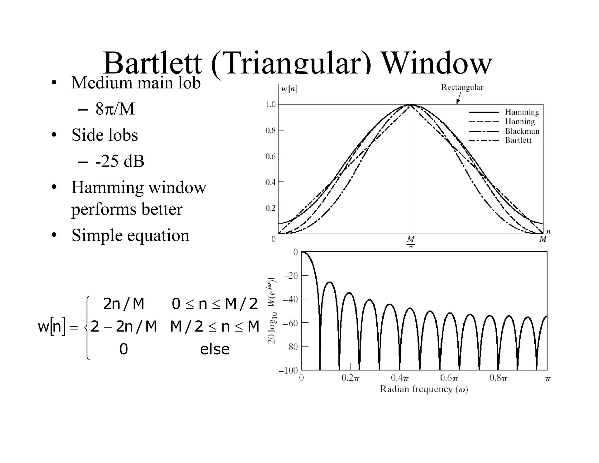
Bartlett (Triangular) Window
else
0
M
n
2
/
M
M
/
n
2
2
2
/
M
n
0
M
/
n
2
n
w
• Medium main lob
– 8/M
• Side lobs
– -25 dB
• Hamming window
performs better
• Simple equation
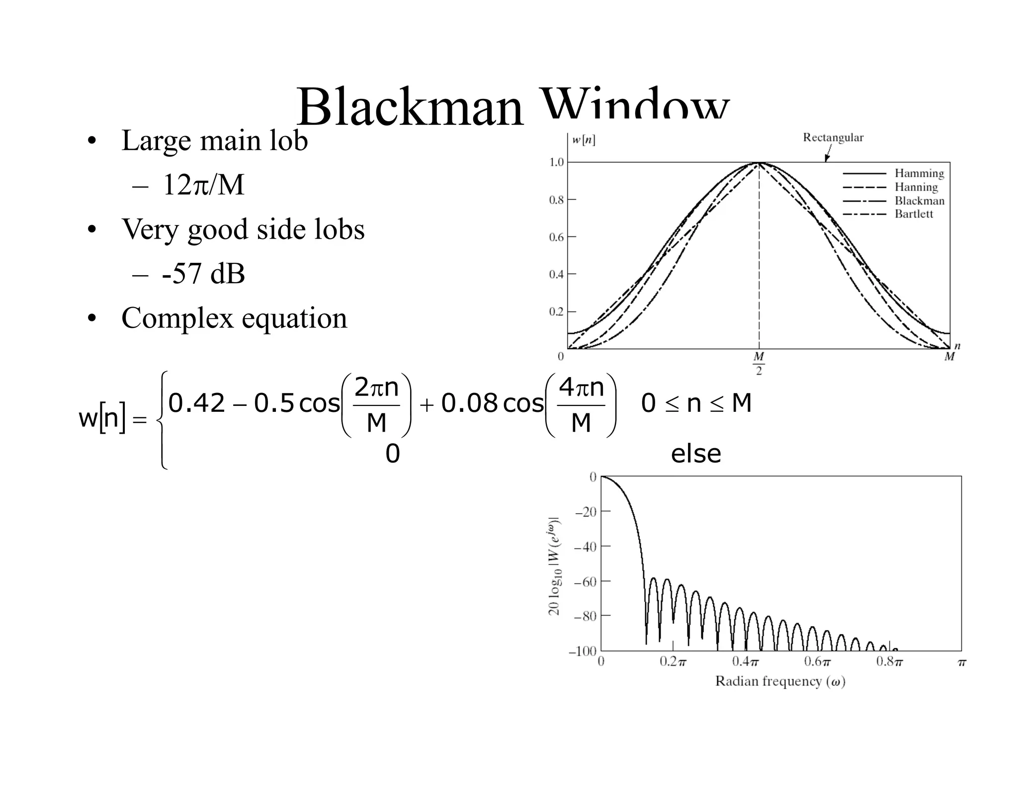
Blackman Window
else
0
M
n
0
M
n
4
cos
08
.
0
M
n
2
cos
5
.
0
42
.
0
n
w
• Large main lob
– 12/M
• Very good side lobs
– -57 dB
• Complex equation
150.
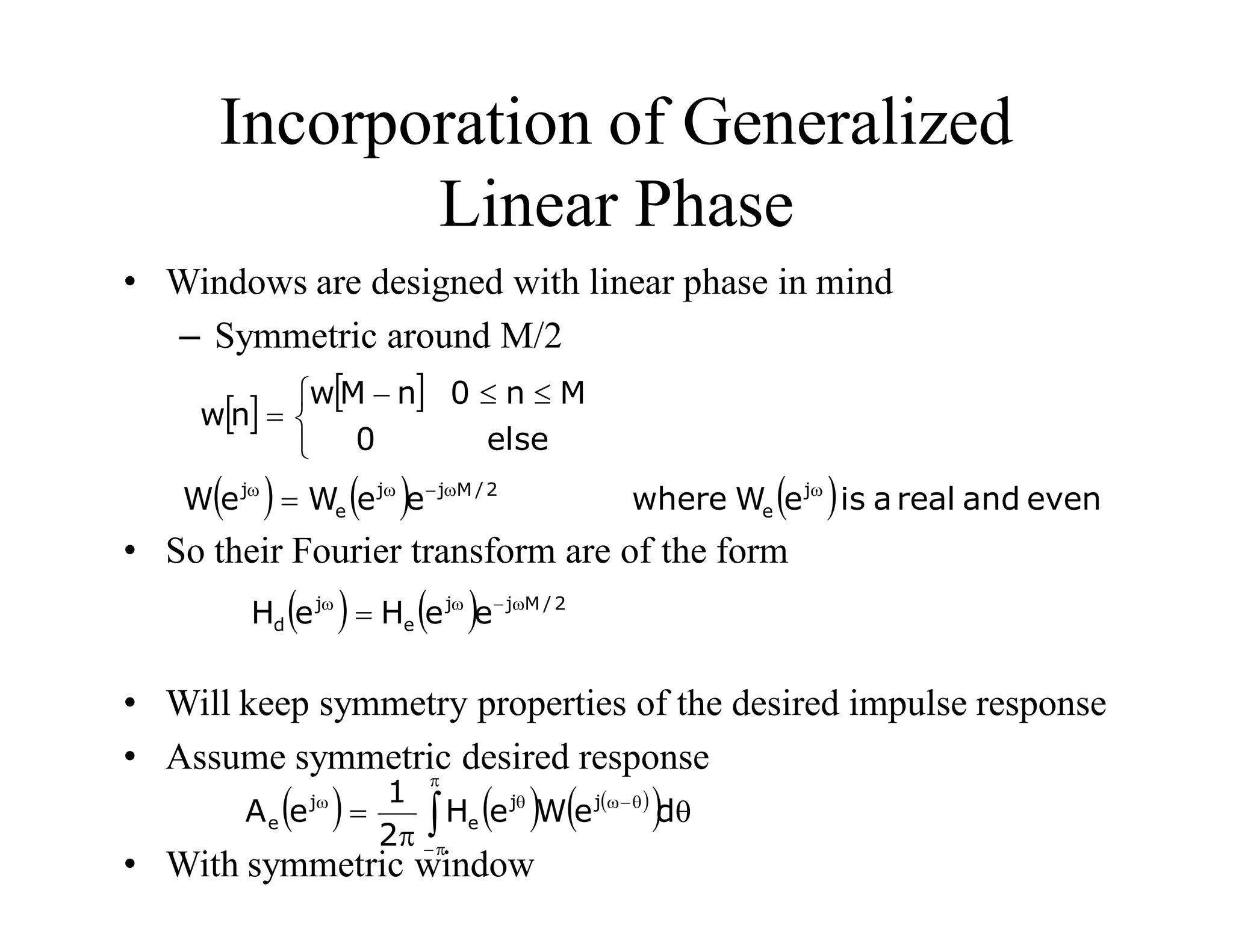
Incorporation of Generalized
LinearPhase
• Windows are designed with linear phase in mind
– Symmetric around M/2
• So their Fourier transform are of the form
• Will keep symmetry properties of the desired impulse response
• Assume symmetric desired response
• With symmetric window
else
0
M
n
0
n
M
w
n
w
even
and
real
a
is
e
W
where
e
e
W
e
W j
e
2
/
M
j
j
e
j w
w
w
w
2
/
M
j
j
e
j
d e
e
H
e
H w
w
w
w
w
d
e
W
e
H
2
1
e
A j
j
e
j
e
151.
Linear-Phase Low passfilter
• Desired frequency response
• Corresponding impulse
response
• Desired response is even
symmetric, use symmetric
window
w
w
w
w
w
w
c
c
2
/
M
j
j
lp
0
e
e
H
2
/
M
n
2
/
M
n
sin
n
h c
lp
w
n
w
2
/
M
n
2
/
M
n
sin
n
h c
w
152.
152
Kaiser Window FilterDesign
Method
• Parameterized equation
forming a set of windows
– Parameter to change
main-lob width and side-
lob area trade-off
– I0(.) represents zeroth-
order modified Bessel
function of 1st kind
else
0
M
n
0
I
2
/
M
2
/
M
n
1
I
n
w
0
2
0
153.
Determining Kaiser Window
Parameters
•Given filter specifications Kaiser developed empirical
equations
– Given the peak approximation error or in dB as A=-
20log10
– and transition band width
• The shape parameter should be
• The filter order M is determined approximately by
21
A
0
50
A
21
21
A
07886
.
0
21
A
5842
.
0
50
A
7
.
8
A
1102
.
0
4
.
0
p
s w
w
w
w
285
.
2
8
A
M
154.
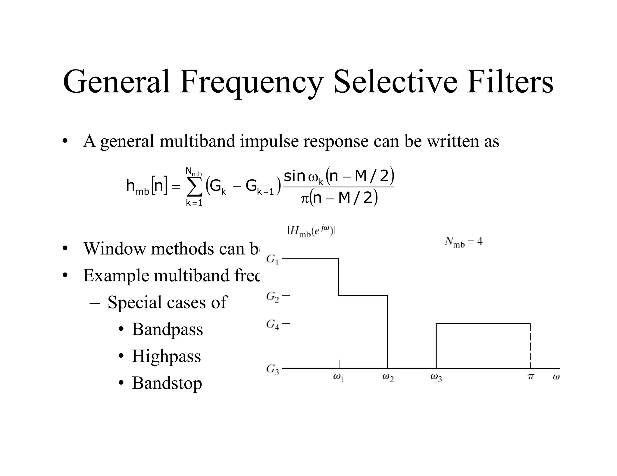
General Frequency SelectiveFilters
• A general multiband impulse response can be written as
• Window methods can be applied to multiband filters
• Example multiband frequency response
– Special cases of
• Bandpass
• Highpass
• Bandstop
w
mb
N
1
k
k
1
k
k
mb
2
/
M
n
2
/
M
n
sin
G
G
n
h
Digital
• Storing informationoften in a series of 1’s and 0’s or binary numbers.
The process can be used to do calculations or sending pulses to
regulate instrumentation or other electronic equipment turning it
on/off or regulating the use of materials such as the flow of liquid
through a valve. In instrumentation and process control this
accomplished by concerting an analogue signal into a digital signal to
control the process. A non-electronic example would be smoke signals
or a beacon.
162.
Analogue
• An analogor analogue signal is any continuously variable signal. It
differs from a digital signal in that small fluctuations in the signal are
meaningful within a given scale range from a small to large signal.
Analog is usually thought of in an electrical context, however
mechanical, pneumatic, hydraulic, and other systems may also use
analog signals.
• A great example of an analogue device is a Wrist Watch with hands
that move.
163.
Binary
• Having thebase of 2 for number system with two digits 0 and 1. Basis
of electronic signal signals used in computers. Creates two states for
the binary signal on or off, 0 being off and 1 being on. There is no
state in between the device is either on or off. Often referred to as
Boolean Logic
164.
Microprocessor
• A siliconbased processing chip or logic chip designed as the heart of
the computer, contains all the necessary information to run a computer
speed measured in megahertz (MHz) or gigahertz (GHz). These chips
have areas for comparing numbers or doing calculations called
registers.
• Good example: Digital Clocks and Wrist Watches
165.
Fuzzy Logic
• Theability of a machine to answer questions that are not yes or no
questions. Fuzzy logic use 0 and 1 as the extremes of yes and no but
answers the degrees of maybe. Fuzzy logic works much closers to that
of the human brain. It is subset of Boolean logic use to fill the
concepts of a partial truth. An example of such is a half full glass of
water is .50 of full.
166.
Neural System
• Ininformation technology, a neural network is a system of programs
and data structures that approximates the operation of the human
brain. A neural network usually involves a large number of processors
operating in parallel, each with its own small sphere of knowledge and
access to data in its local memory.
• Good example: Joystick for a computer game
167.
Sensors
• Devices suchas a photocell that respond to a signal or stimulus. A
device that measures or detects a real-world condition, such as
motion, heat or light and converts the condition into an analog or
digital representation. These devices are use in manufacturing plants
to tell how many items are in a package such as the example CD’s to
fill a container for packaging or to the number of containers fill case
for shipment.
• Good examples: motion detectors and burglar alarms
168.
Actuators
• One thatactivates, especially a device responsible for actuating a
mechanical device, such as one connected to a computer by a sensor
link.
• An actuator is the mechanism by which an agent acts upon an
environment. The agent can be either an artificial or any other
autonomous being (human, other animal, etc).
• Examples: human hand, leg, arm, Part Picking Robot, Switches
169.
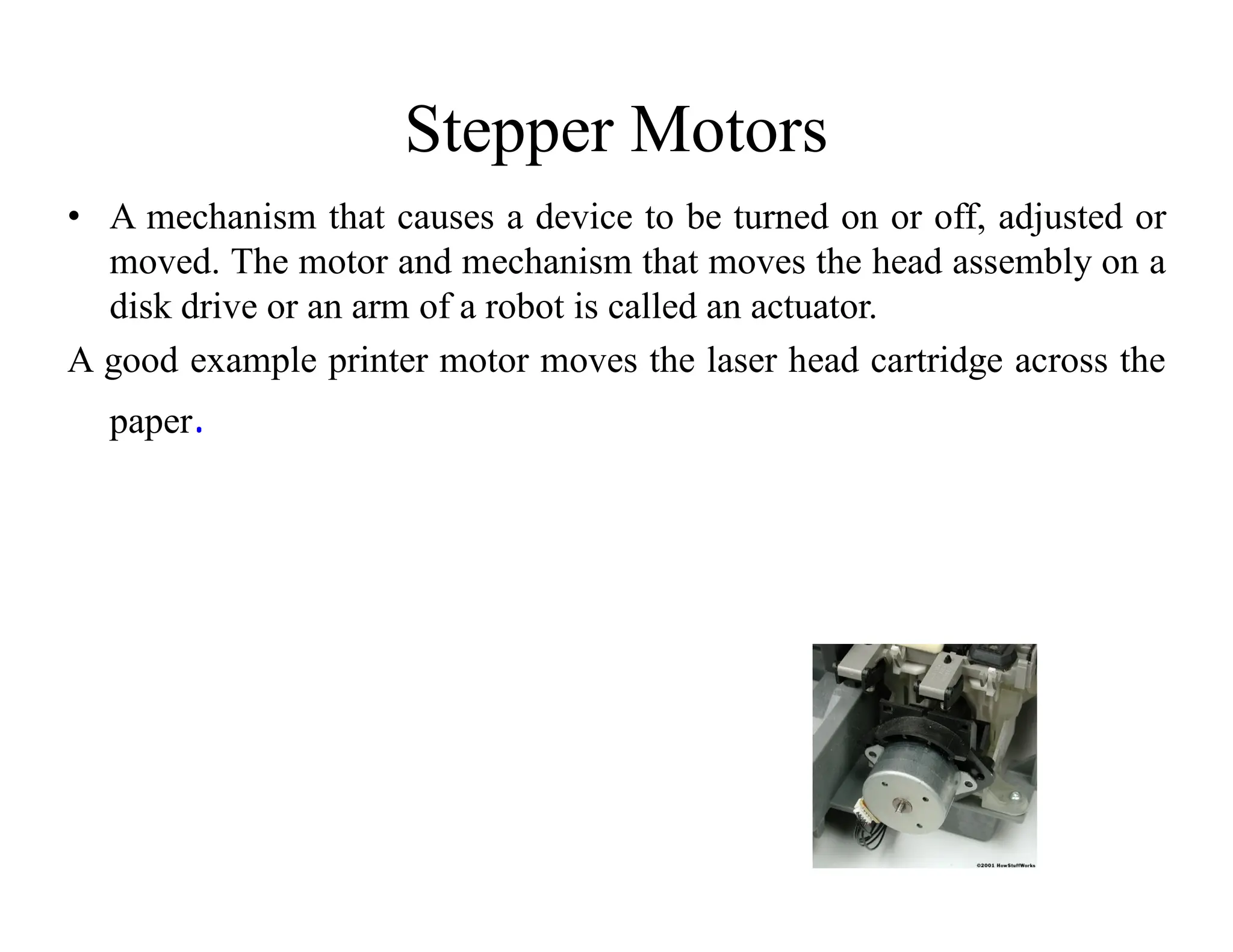
Stepper Motors
• Amechanism that causes a device to be turned on or off, adjusted or
moved. The motor and mechanism that moves the head assembly on a
disk drive or an arm of a robot is called an actuator.
A good example printer motor moves the laser head cartridge across the
paper.
170.
Synchro Motor
• Atype of rotary transformer fixed to rotor which attached to a motor
and can be adjusted. The current is adjusted to keep the rotor and
motor operating at a synchronized speed. The result of this action
causes the parts to work in unison.
• Good Examples: the gun turret on a naval destroyer and the film and
sound of older movies before microelectronics.
171.
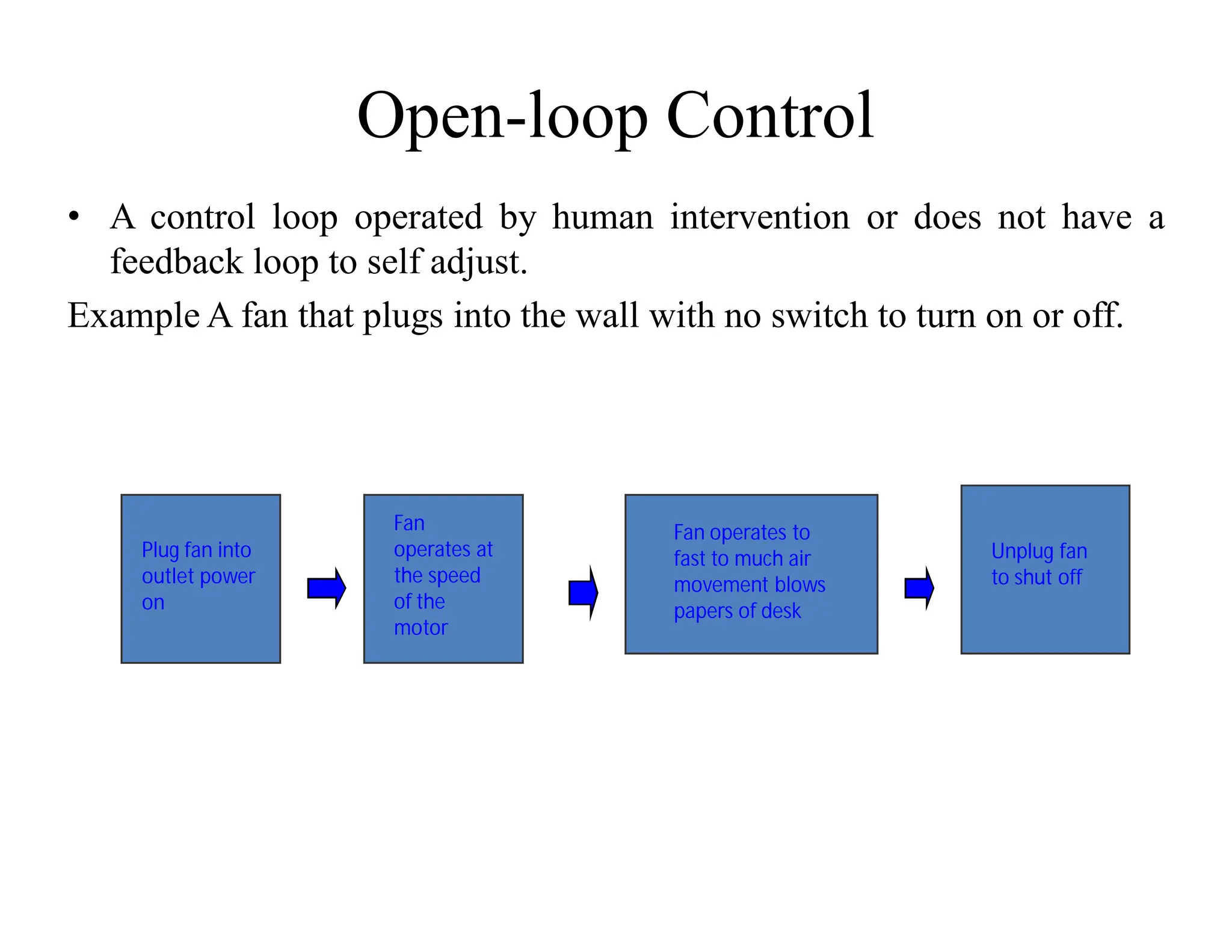
Open-loop Control
• Acontrol loop operated by human intervention or does not have a
feedback loop to self adjust.
Example A fan that plugs into the wall with no switch to turn on or off.
Plug fan into
outlet power
on
Fan
operates at
the speed
of the
motor
Unplug fan
to shut off
Fan operates to
fast to much air
movement blows
papers of desk
172.
Closed-loop Control
• Acontrol-loop operated by a feedback loop allowing self adjusting of
the loop.” A mechanical, optical, or electronic system that is used to
maintain a desired output.”
• Good example: Fan with a switch to allow the speed to be changed
Fan
plugged
in
Fan
turned
on
Fan is
to fast
papers
blow
around
Switch
turned
down to
lower fan
speed
Fan works
fine papers
do not blow
around
Fan
speed
can be
adjusted
or turned
off
173.
Instrumentation
• Instrumentation isdefined as "the art and science of measurement and
control". Instrumentation is used to refer to the field in which
Instrument technicians and engineers work. Instrumentation also can
refer to the available methods of measurement and control
• Good example: the gauges that control the boilers for the school
heating system
1. Basic Definitions
Database:A collection of related data.
Data: Known facts that can be recorded and have an
implicit meaning.
Mini-world: Some part of the real world about which
data is stored in a database. For example, consider
student names, student grades and transcripts at a
university.
176.
Database Management System(DBMS): A software package/
system to facilitate the creation and maintenance of a
computerized database.
It
• defines (data types, structures, constraints)
• construct (storing data on some storage medium
controlled by DBMS)
• manipulate (querying, update, report generation) databases
for various applications.
Database System: The DBMS software together with the data
itself. Sometimes, the applications are also included.
178.
2.File Processing andDBMS
File Systems :
– Store data over long periods of time
– Store large amount of data
However :
– No guarantee that data is not lost if not backed up
– No support to query languages
– No efficient access to data items unless the location is
known
– Application depends on the data definitions (structures)
– Change to data definition will affect the application
programs
– Single view of the data
– Separate files for each application
– Limited control to multiple accesses
- Data viewed as physically stored
179.
3. Main Characteristicsof Database
Technology
- Self-contained nature of a database system: A DBMS catalog
stores the description (structure, type, storage format of each
entities) of the database. The description is called meta-data).
This allows the DBMS software to work with different databases.
- Insulation between programs and data: Called program-data
independence. Allows changing data storage structures and
operations without having to change the DBMS access programs.
- Data Abstraction: A data model is used to hide storage details
and present the users with a conceptual view of the database;
does not include how data is stored and how the operations are
implemented.
-
180.
• Support ofmultiple views of the data: Each user may see a
different view of the database, which describes only the
data of interest to that user.
• Sharing of Data and Multiple users
181.
DBA – DatabaseAdministrator
- Responsible for authorizing access to the database,
coordinating, monitoring its use, acquiring hardware,
software needed.
Database designers
- Responsible for identifying the data to be stored, storage
structure to represent and store data. This is done by a team
of professionals in consultation with users, and
applications needed.
182.
4. Additional Benefitsof Database
Technology
- Controlling redundancy in data storage and in development and
maintenance efforts.
- Sharing of data among multiple users.
- Restricting unauthorized access to data.
- Providing multiple interfaces to different classes of users.
- Representing complex relationships among data.
- Enforcing integrity constraints on the database.
- Providing backup and recovery services.
- Potential for enforcing standards.
- Flexibility to change data structures.
- Reduced application development time.
- Availability of up-to-date information.
• Economies of scale.
183.
5 When notto use a DBMS
Main inhibitors (costs) of using a DBMS:
- High initial investment and possible need for additional hardware.
- Overhead for providing generality, security, recovery, integrity,
and concurrency control.
When a DBMS may be unnecessary:
- If the database and applications are simple, well defined, and not
expected to change.
- If there are stringent real-time requirements that may not be met
because of DBMS overhead.
- If access to data by multiple users is not required.
When no DBMS may suffice:
- If the database system is not able to handle the complexity of data
because of modeling limitations
- If the database users need special operations not supported by the
DBMS.
184.
6. Data Models
DataModel: A set of concepts to describe the structure (data
types, relationships) of a database, and certain constraints that
the database should obey.
Data Model Operations: Operations for specifying database
retrievals and updates by referring to the concepts of the data
model.
185.
DBMS Languages
Data DefinitionLanguage (DDL): Used by the DBA and
database designers to specify the conceptual schema of a
database.
In many DBMSs, the DDL is also used to define internal and
external schemas (views). In some DBMSs, separate storage
definition language (SDL) and view definition language
(VDL) are used to define internal and external schemas.
Data Manipulation Language (DML): Used to specify database
retrievals and updates.
-DML commands (data sublanguage) can be embedded in a
general-purpose programming language (host language), such
as COBOL, PL/1 or PASCAL.
- Alternatively, stand-alone DML commands can be applied
directly (query language).
186.
High Level ornon-Procedural DML – Describes what data to
be retrieved rather than how to retrieve.
- Process many records at a time
- SQL
Low Level or Procedural DML – It needs constructs for
both, what to retrieve and what to
retrieve
- Uses looping etc. like programming languages
Only access one record at a time
187.
DBMS Interfaces
- Stand-alonequery language interfaces.
- Programmer interfaces for embedding DML in programming
languages:
- Pre-compiler Approach
- Procedure (Subroutine) Call Approach
- User-friendly interfaces:
- Menu-based
- Graphics-based (Point and Click, Drag and Drop etc.)
- Forms-based
- Natural language
- Combinations of the above
- Speech as Input (?) and Output
- Web Browser as an interface
-
188.
Classification of DBMSs
Basedon the data model used:
- Traditional: Relational, Network, Hierarchical.
- Emerging: Object-oriented, Object-relational.
Other classifications:
- Single-user (typically used with micro- computers) vs.
multi-user (most DBMSs).
- Centralized (uses a single computer with one database)
vs. distributed (uses multiple computers, multiple databases)
Distributed Database Systems have now come to be known as
client server based database systems because they do not
support a totally distributed environment, but rather a set
of database servers supporting a set of clients.
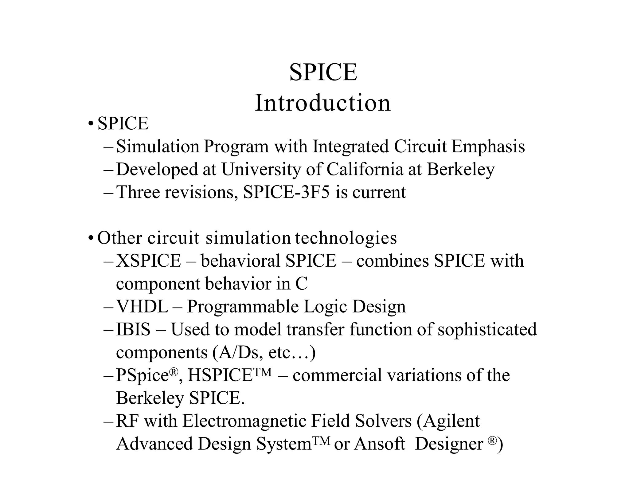
• SPICE
–Simulation Programwith Integrated Circuit Emphasis
–Developed at University of California at Berkeley
–Three revisions, SPICE-3F5 is current
• Other circuit simulation technologies
–XSPICE – behavioral SPICE – combines SPICE with
component behavior in C
–VHDL – Programmable Logic Design
–IBIS – Used to model transfer function of sophisticated
components (A/Ds, etc…)
–PSpice®, HSPICETM – commercial variations of the
Berkeley SPICE.
–RF with Electromagnetic Field Solvers (Agilent
Advanced Design SystemTM or Ansoft Designer ®)
SPICE
Introduction
191.
SPICE Primer
• SPICECircuit
– Built by creating a netlist of native SPICE
primitive models.
– Netlist is a text file that lists all connections and
model information.
– Schematic File
• Vendor specific
• May include package, footprint, and
additional information
– SPICE adds analysis commands on top of
SPICE file allowing a SPICE simulation to
extract information out of circuit (Transient,
AC, Monte Carlo etc…)
• Variety of native SPICE components:
– Resistors, Capacitors, Inductors, Sources,
Transistors, etc…
192.
Advantages to Using
SPICEwith Virtual Instrumentation
Mathematical capabilities of SPICE to accurately model
complex circuits and devices
- AND –
Measurement capabilities of Virtual Instrumentation
(such as data collection, automation, testing, etc)
SPICE
Schematic,Simulation,Analysis
Virtual Prototype
Testing
Measurements
Physical Measurements
Comparison between simulation data
and measurements is simplified
VI Software
Virtual Measurements
193.
Simulation and Measurementsfor Design
Engineers
LogicAnalyzer
Function Generator
Scope
Power Supply
DMM
•How do you effectively compare test
bench data with simulation data?
•How can you bring in measurement data
into simulation?
•Is there anyway to perform simulations,
compare results and optimize the design
automatically?
194.
Multisim and LabVIEWIntegration
1 .Build Circuit and
Simulate in Multisim
2. Use LabVIEW to
generate realistic test
and/or stimulus waveforms
3. Create Measurements in
LabVIEW Reflective of real tests
done during testing
4. Once Hardware Prototype is
completed, use same measurements
for validation testing.
5. Key Step: Compare Measurements
and Simulation Data for Improving
Design Functionality and Performance
195.
In this chapterwe describe a general process for designing a control
system.
A control system consisting of interconnected components is designed
to achieve a desired purpose. To understand the purpose of a control
system, it is useful to examine examples of control systems through
the course of history. These early systems incorporated many of the
same ideas of feedback that are in use today.
Modern control engineering practice includes the use of control
design strategies for improving manufacturing processes, the
efficiency of energy use, advanced automobile control, including
rapid transit, among others.
We also discuss the notion of a design gap. The gap exists between
the complex physical system under investigation and the model used
in the control system synthesis.
Development of Control system
196.
System – Aninterconnection of elements and devices for a desired
purpose.
Control System – An interconnection of components forming a
system configuration that will provide a desired response.
Process – The device, plant, or
system under control. The input
and output relationship
represents the cause-and-effect
relationship of the process.
197.
Control System
• Controlis the process of causing a system variable to conform
to some desired value.
• Manual control Automatic control (involving machines
only).
• A control system is an interconnection of components forming
a system configuration that will provide a desired system
response.
Control
System
Output
Signal
Input
Signal
Energy
Source
198.
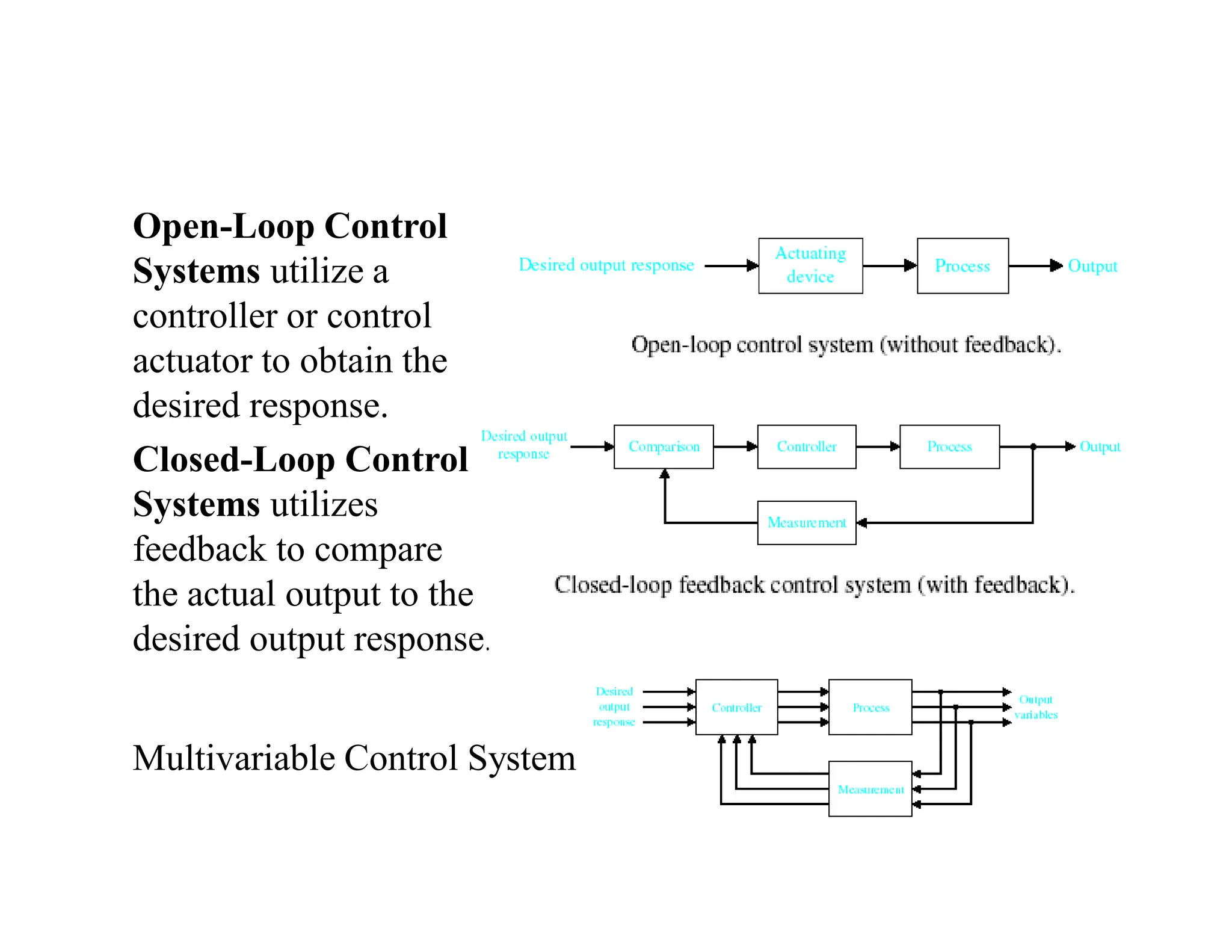
Multivariable Control System
Open-LoopControl
Systems utilize a
controller or control
actuator to obtain the
desired response.
Closed-Loop Control
Systems utilizes
feedback to compare
the actual output to the
desired output response.
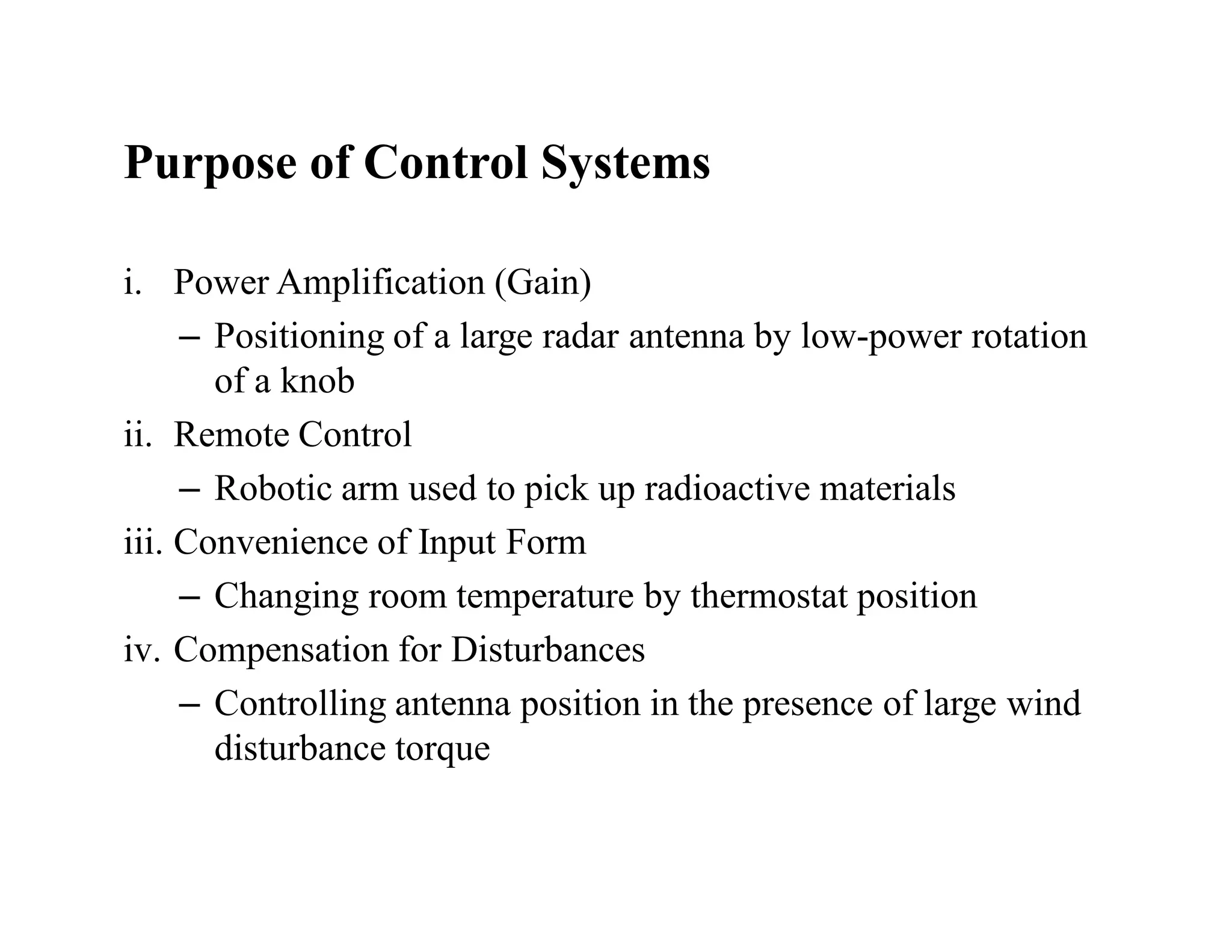
Purpose of ControlSystems
i. Power Amplification (Gain)
– Positioning of a large radar antenna by low-power rotation
of a knob
ii. Remote Control
– Robotic arm used to pick up radioactive materials
iii. Convenience of Input Form
– Changing room temperature by thermostat position
iv. Compensation for Disturbances
– Controlling antenna position in the presence of large wind
disturbance torque
203.
Historical Developments
i. AncientGreece (1 to 300 BC)
– Water float regulation, water clock, automatic oil lamp
ii. Cornellis Drebbel (17th century)
– Temperature control
iii. James Watt (18th century)
– Flyball governor
iv. Late 19th to mid 20th century
– Modern control theory
204.
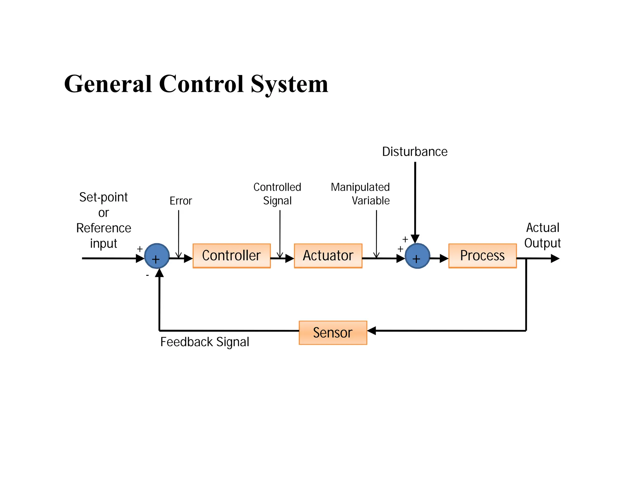
Control System Components
i.System, plant or process
– To be controlled
ii. Actuators
– Converts the control signal to a power signal
iii. Sensors
– Provides measurement of the system output
iv. Reference input
– Represents the desired output
205.
General Control System
Sensor
ActuatorProcess
Controller +
+
Set-point
or
Reference
input
Actual
Output
Error
Controlled
Signal
Disturbance
Manipulated
Variable
Feedback Signal
+
-
+
+
206.
Image acquisition andprocessing-
Image Processing Fields
• Computer Graphics: The creation of images
• Image Processing: Enhancement or other manipulation of the
image
• Computer Vision: Analysis of the image content
207.
Image Processing Fields
Input/ Output Image Description
Image Image Processing Computer Vision
Description Computer Graphics AI
Sometimes, Image Processing is defined as “a
discipline in which both the input and output
of a process are images
But, according to this classification, trivial
tasks of computing the average intensity of an
image would not be considered an image
processing operation
208.
Computerized Processes Types
•Mid-Level Processes:
– Inputs, generally, are images. Outputs are attributes
extracted from those images (edges, contours, identity of
individual objects)
– Tasks:
• Segmentation (partitioning an image into regions or
objects)
• Description of those objects to reduce them to a form
suitable for computer processing
• Classifications (recognition) of objects
209.
Digital Image Definition
•An image can be defined as a two-dimensional function f(x,y)
• x,y: Spatial coordinate
• F: the amplitude of any pair of coordinate x,y, which is called
the intensity or gray level of the image at that point.
• X,y and f, are all finite and discrete quantities.
210.
Fundamental Steps inDigital Image Processing:
Image
Acquisition
Image
Restoration
Morphological
Processing
Segmentation
Object
Recognition
Image
Enhancement Representation
& Description
Problem Domain
Colour Image
Processing
Image
Compression
Wavelets &
Multiresolution
processing
Knowledge Base
Outputs of these processes generally are images
Outputs
of
these
processes
generally
are
image
attributes
211.
Fundamental Steps inDIP:
(Description)
Step 1: Image Acquisition
The image is captured by a sensor (eg. Camera), and digitized
if the output of the camera or sensor is not already in digital
form, using analogue-to-digital convertor
212.
Fundamental Steps inDIP:
(Description)
Step 2: Image Enhancement
The process of manipulating an image so that the result is
more suitable than the original for specific applications.
The idea behind enhancement techniques is to bring out details
that are hidden, or simple to highlight certain features of
interest in an image.
213.
Fundamental Steps inDIP:
(Description)
Step 3: Image Restoration
- Improving the appearance of an image
- Tend to be mathematical or probabilistic models.
Enhancement, on the other hand, is based on human subjective
preferences regarding what constitutes a “good” enhancement
result.
214.
Fundamental Steps inDIP:
(Description)
Step 4: Colour Image Processing
Use the colour of the image to extract features of interest in an
image
215.
Fundamental Steps inDIP:
(Description)
Step 5: Wavelets
Are the foundation of representing images in various degrees
of resolution. It is used for image data compression.
216.
Fundamental Steps inDIP:
(Description)
Step 6: Compression
Techniques for reducing the storage required to save an image
or the bandwidth required to transmit it.
217.
Fundamental Steps inDIP:
(Description)
Step 7: Morphological Processing
Tools for extracting image components that are useful in the
representation and description of shape.
In this step, there would be a transition from processes that
output images, to processes that output image attributes.
218.
Fundamental Steps inDIP:
(Description)
Step 8: Image Segmentation
Segmentation procedures partition an image into its constituent
parts or objects.
Important Tip: The more accurate the segmentation, the
more likely recognition is to succeed.
219.
Fundamental Steps inDIP:
(Description)
Step 9: Representation and Description
- Representation: Make a decision whether the data should be
represented as a boundary or as a complete region. It is almost
always follows the output of a segmentation stage.
- Boundary Representation: Focus on external shape
characteristics, such as corners and inflections ()اﻧﺤﻨﺎءات
- Region Representation: Focus on internal properties, such
as texture or skeleton ()ھﯿﻜﻠﯿﺔ shape
220.
Fundamental Steps inDIP:
(Description)
Step 9: Representation and Description
- Choosing a representation is only part of the solution for
transforming raw data into a form suitable for subsequent
computer processing (mainly recognition)
- Description: also called, feature selection, deals with
extracting attributes that result in some information of interest.
221.
Fundamental Steps inDIP:
(Description)
Step 10: Knowledge Base
Knowledge about a problem domain is coded into an image
processing system in the form of a knowledge database.
222.
Components of anImage Processing
System
Network
Image displays Computer Mass storage
Hardcopy
Specialized image
processing hardware
Image processing
software
Image sensors
Problem Domain
Typical general-
purpose DIP
system
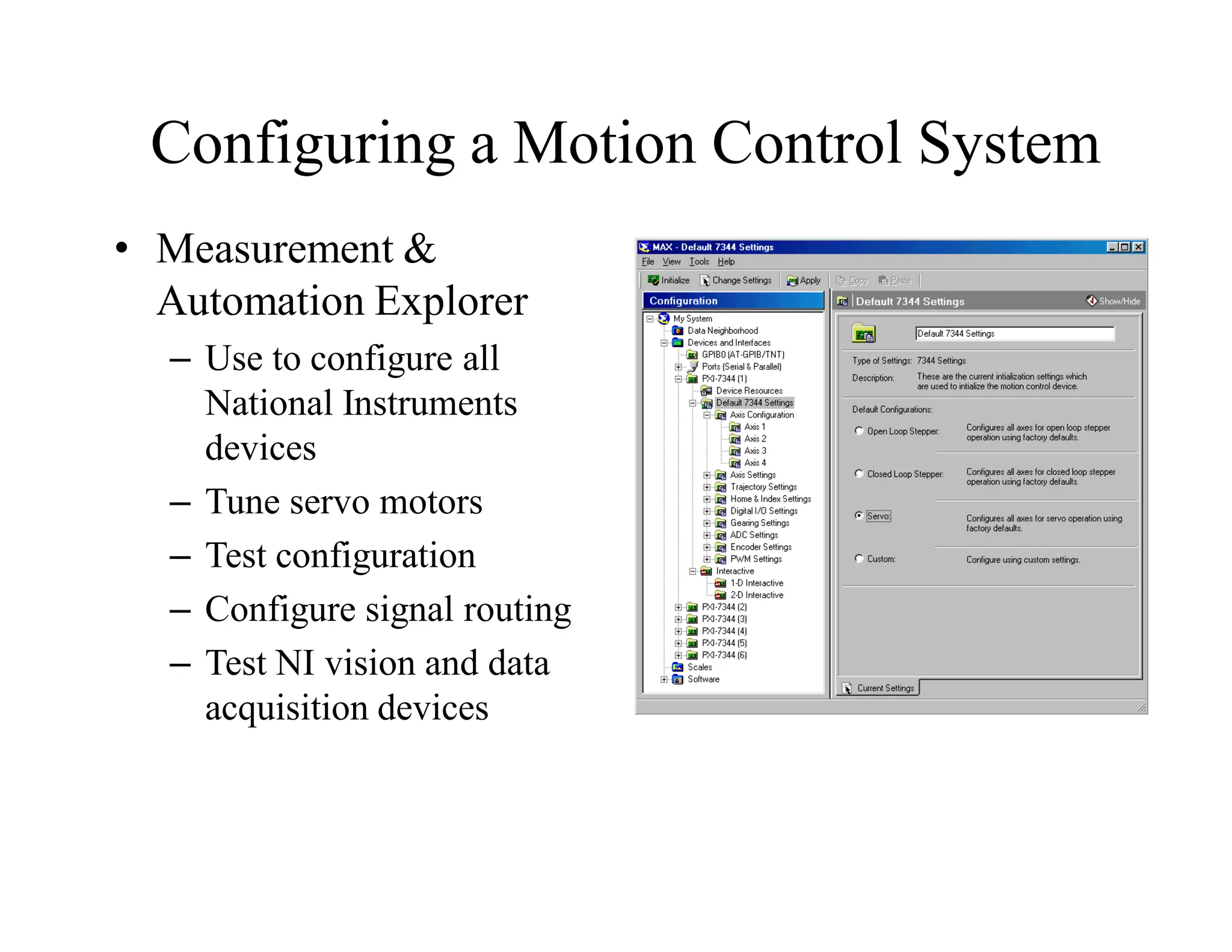
Configuring a MotionControl System
• Measurement &
Automation Explorer
– Use to configure all
National Instruments
devices
– Tune servo motors
– Test configuration
– Configure signal routing
– Test NI vision and data
acquisition devices
227.
NI-Motion Driver Software
•For Windows and LabVIEW Real-Time Systems
– VIs and functions for LabVIEW, Visual Basic, and C
– Measurement and Automation Explorer
• Configuration of motion and other components
• Motor Tuning
• For Non-Windows Systems
– Motion Control Hardware DDK
– Linux and VxWorks drivers from Sensing Systems
(www.sensingsystems.com)
228.
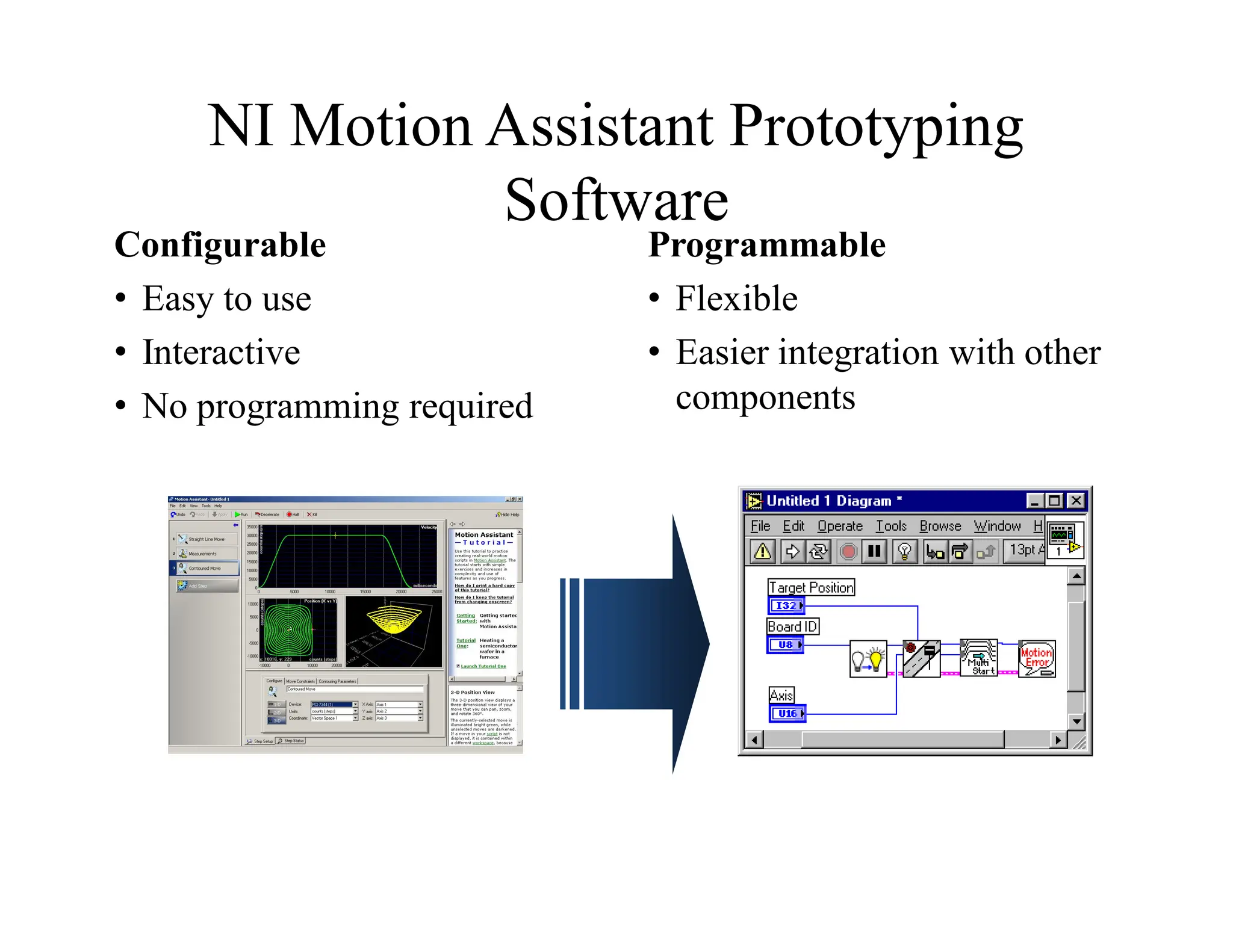
NI Motion AssistantPrototyping
Software
Configurable
• Easy to use
• Interactive
• No programming required
Programmable
• Flexible
• Easier integration with other
components
229.
Purpose of theMotion Controller
• Calculate the trajectories for each commanded move on the
board to prevent host computer interference
• Provide the torque commands to the motor drive or amplifier
• Monitor limits and emergency stops for supervisory control
• Close the PID loop
230.
Motor Drive Requirements
•The motor drive must match the motor technology
– For example, 2-phase stepper motors require 2 phase stepper
motor drives, etc…
• The motor drive must provide adequate:
– Peak current
– Continuous current
– Voltage
231.
NI Motor DriveProducts
• MID series Stepper and Servo drives
– MID-7604/2 four and two axis 1.4 Amp/phase stepper
drive
– MID-7654/2 four and two axis 5 Amp continuous servo
drive
• Universal Motion Interface (UMI) for easy connectivity to 3rd
party drives
• See Drive Advisor at ni.com/motion/advisors for info on third
party drives
232.
• Computer purchasedas part of some other piece of
equipment
– Typically dedicated software (may be user customizable)
– Often replaces previously electromechanical
components
– Often no “real” keyboard
– Often limited display or no general purpose display
device
• But, every system is unique there are always
exceptions
What is an Embedded System?
233.
An Embedded ControlSystem
Designer's View
• Measured by:
Cost, Time to market, Cost, Functionality, Cost & Cost.
234.
What is OPC
•A “real world” application of object technology used to devise
a standard communication system to enable industrial plant
floor devices and business software applications to
communicate via a standard common protocol.
235.
Communication
• Communication andintegration of plant information systems:
– Many different plant floor devices and process control
software applications from many different vendors
– Business Information and Management software
A Better Way:OPC
• The OPC Standard now places the burden on hardware
vendors to develop a single OPC “driver” (server) that is
responsible for data collection and distribution for their
device(s).
• Provide data to clients in a standard manor.
238.
Client / ServerRelationship
• Software developers can now write clients that can
communicate with hardware OPC servers using a common,
efficient protocol
OPC Client #1
OPC
Server
Vendor A
OPC
Server
Vendor C
OPC
Server
Vendor B
OPC Client #2
OPC Client #3
239.
Technology (TLA Guide)
•COM - Component Object Model
– Provides objects as reusable, binary components
– objects “expose” a set of interfaces that client applications
can use to access the object’s services.
– Implementation is encapsulated behind interfaces (allows
object to change without requiring client recompilation)
240.
Technology (continued)
• DCOM- Distributed Component Object Model
– remote objects appear to be local
• OLE - Object Linking and Embedding
– based on COM (e.g. an OLE object implements certain
COM interfaces)
– provides integration among applications
241.
Technology (continued)
• OLEAutomation
– Allows components to easily be used by high level
custom programs (e.g. written in VB or VBA)
– Set of special COM interfaces
• automation or ActiveX objects implement these
“automation” interfaces
– Automation Controllers
• Clients that can integrate those objects
242.
OPC and COM
•OPC Specifications contain defined COM interfaces
• Server and Client Interfaces
– Data Access
– Historical Data
– Alarms and Events
– etc.
• Implementation and development
What is SCADA?
Supervisory Control and Data Acquisition
Supervisory
Operator/s, engineer/s, supervisor/s, etc
Control
Monitoring
Limited
Telemetry
Remote/Local
Data acquisition
Access and acquire information or data from the
equipment
Sends it to different sites through telemetry
Analog / Digital
245.
Elements of SCADA
Elementsof a SCADA system
Sensors and actuators
RTUs/PLCs
Communication
MTU
Front End Processor
SCADA server
Historical/Redundant/Safety Server
HMI computer
HMI software
246.
SCADA server
SCADA Server
It can be a Web server
Data logging
Analyzing data
Serve the clients through a firewall
Clients connected in the corporation or connected
outside through internet
Real-time decision maker
Asks RTU for information
247.
HMI Computer
Human MachineInterface Computer
Access on the SCADA Server
Control the system
Operator Interface
Software
User friendly
Programmable (C, C++)
248.
DCS
DCS – DistributedControl System
Process oriented – tendency to do something
Not event oriented – does not depend on
circumstances
Local control over the devices
Subordinate to SCADA


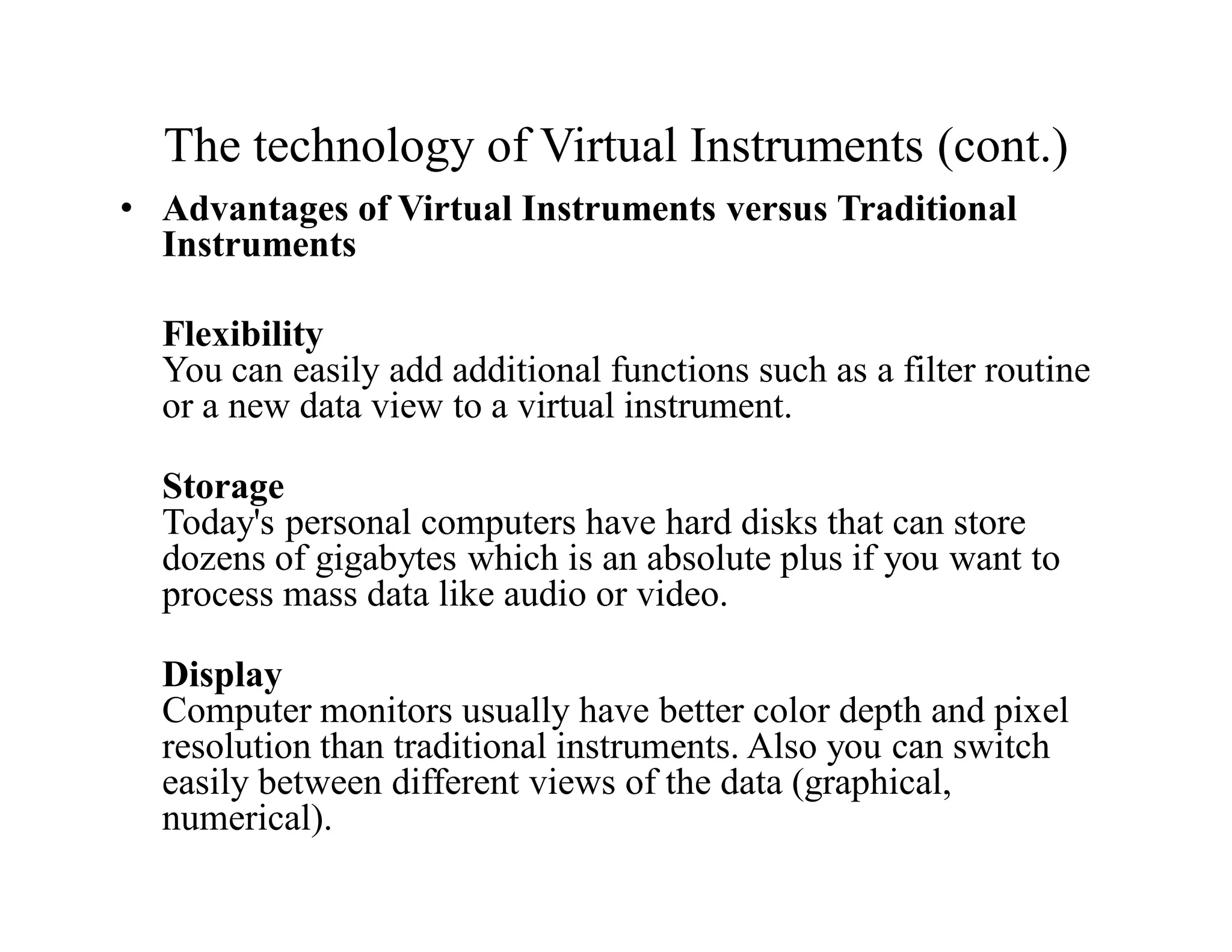


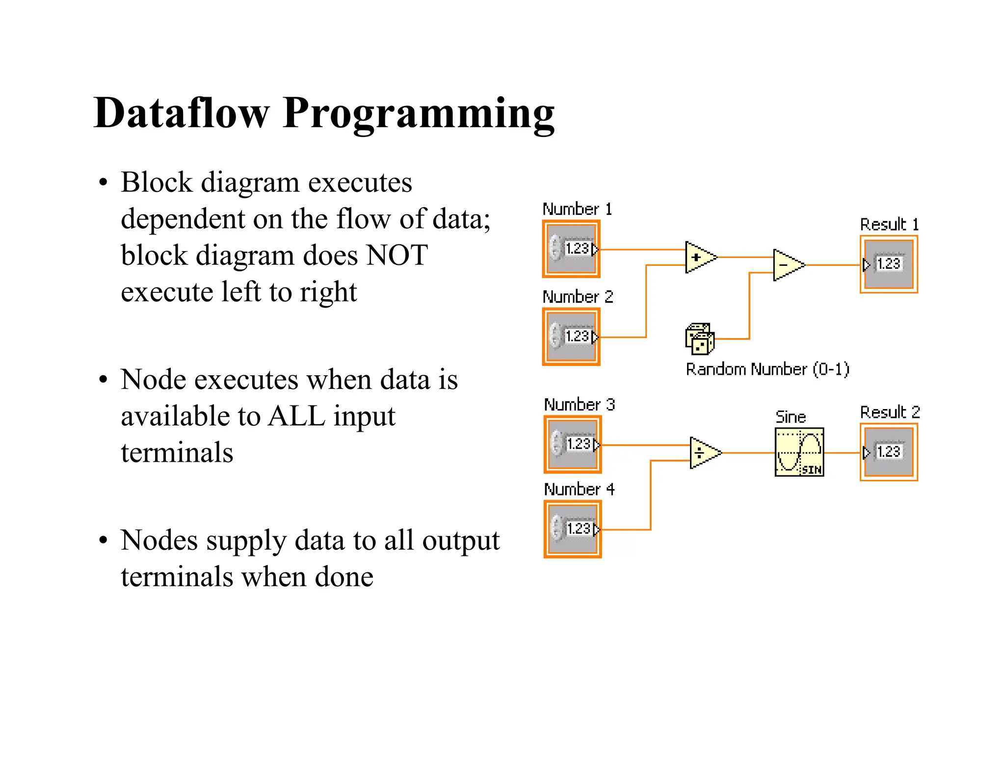
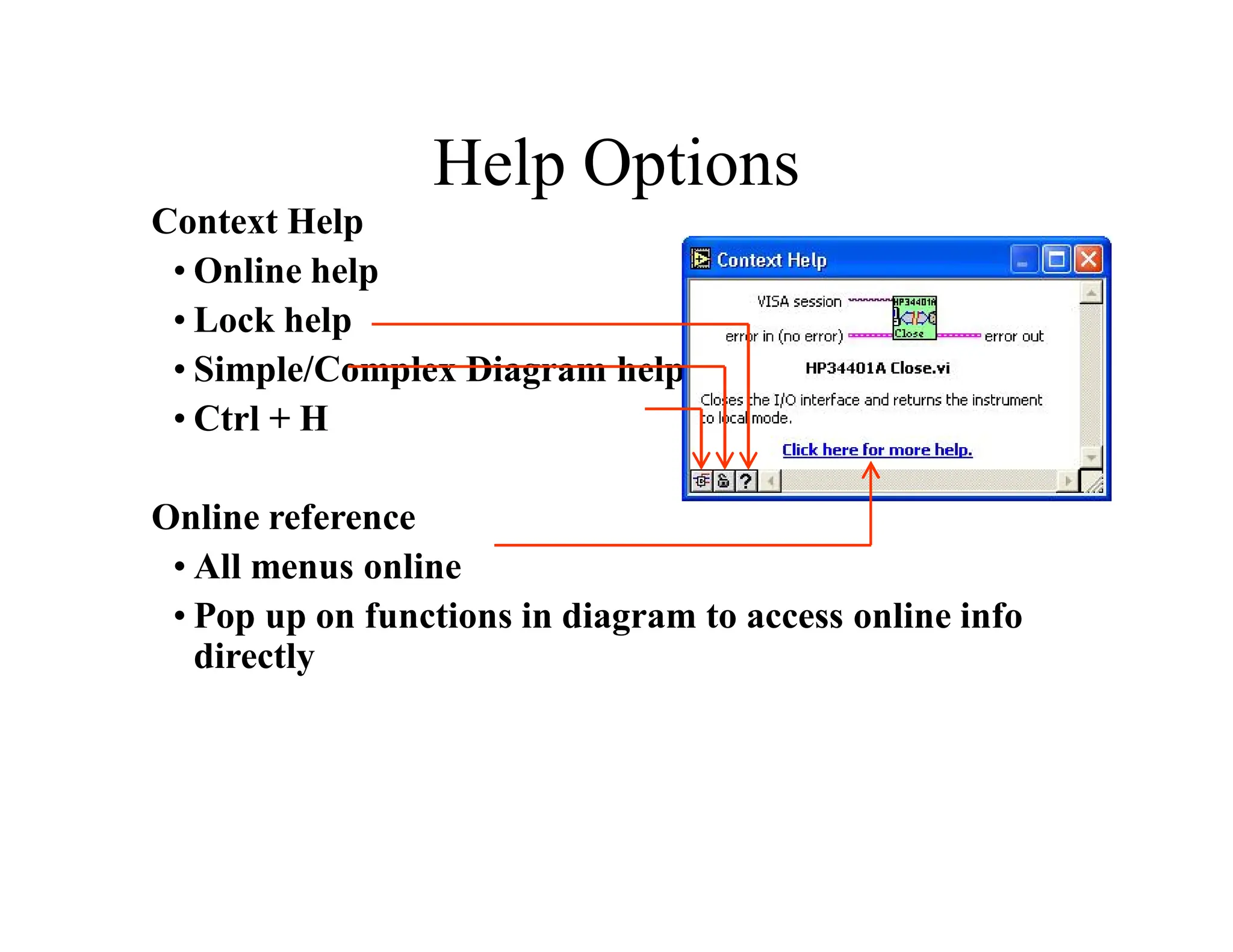


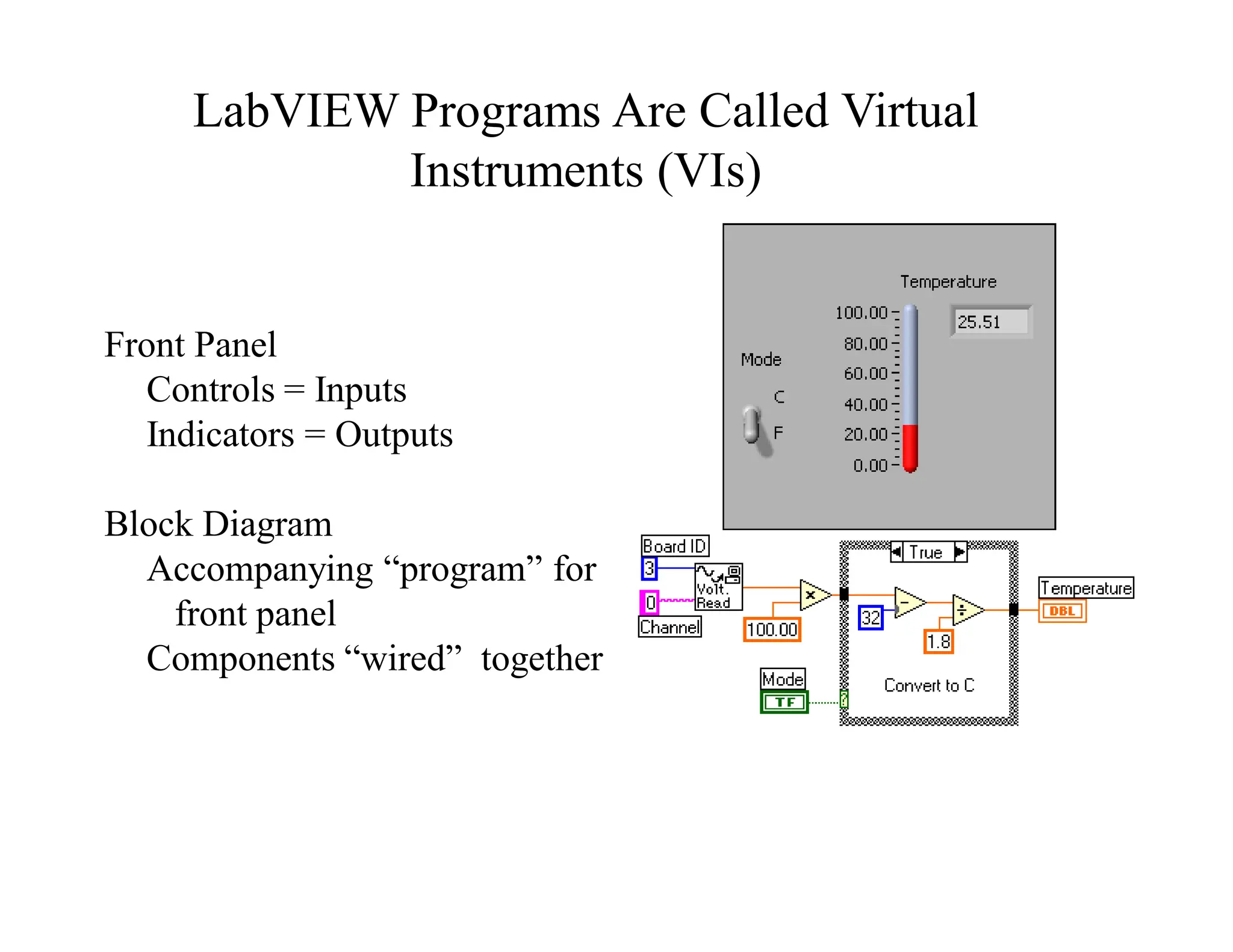
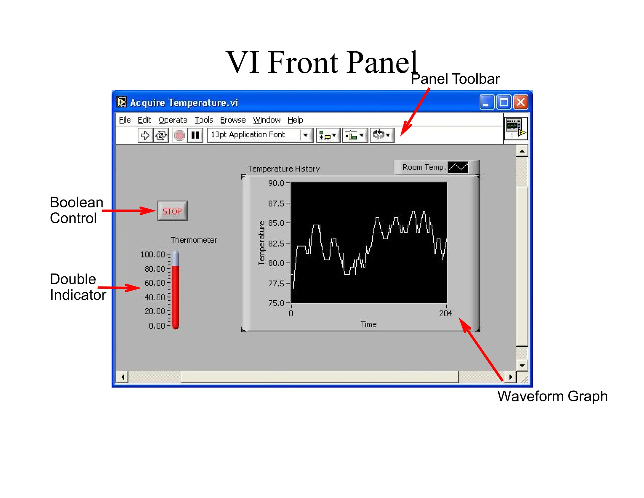


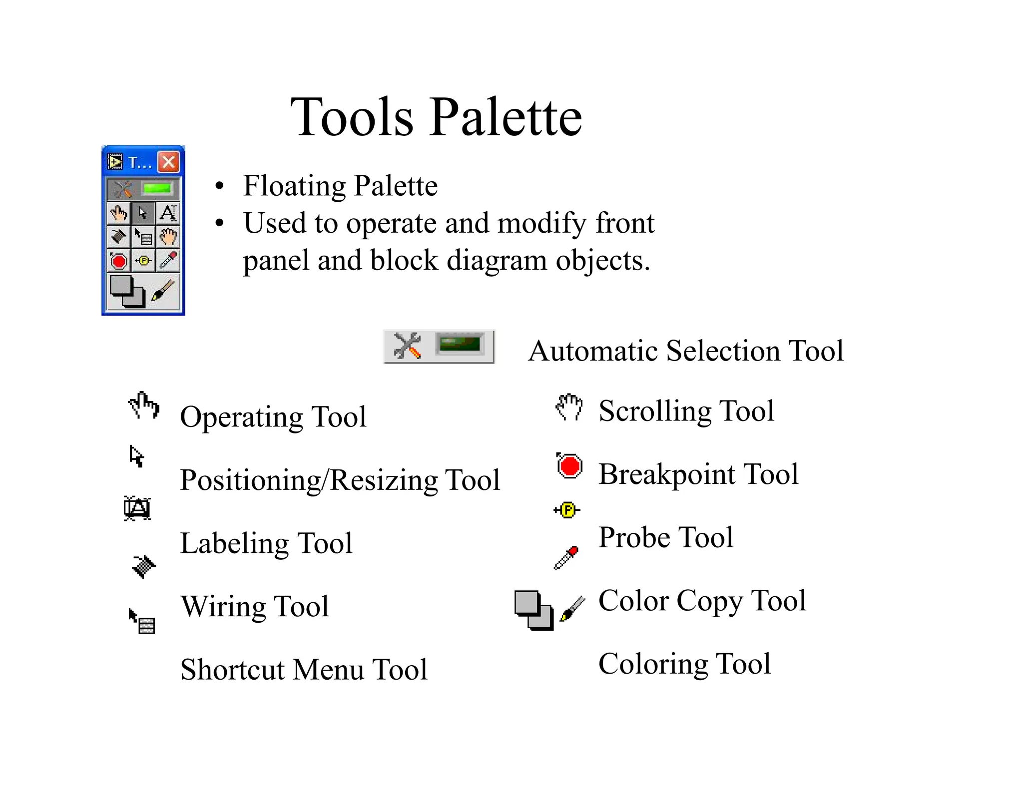


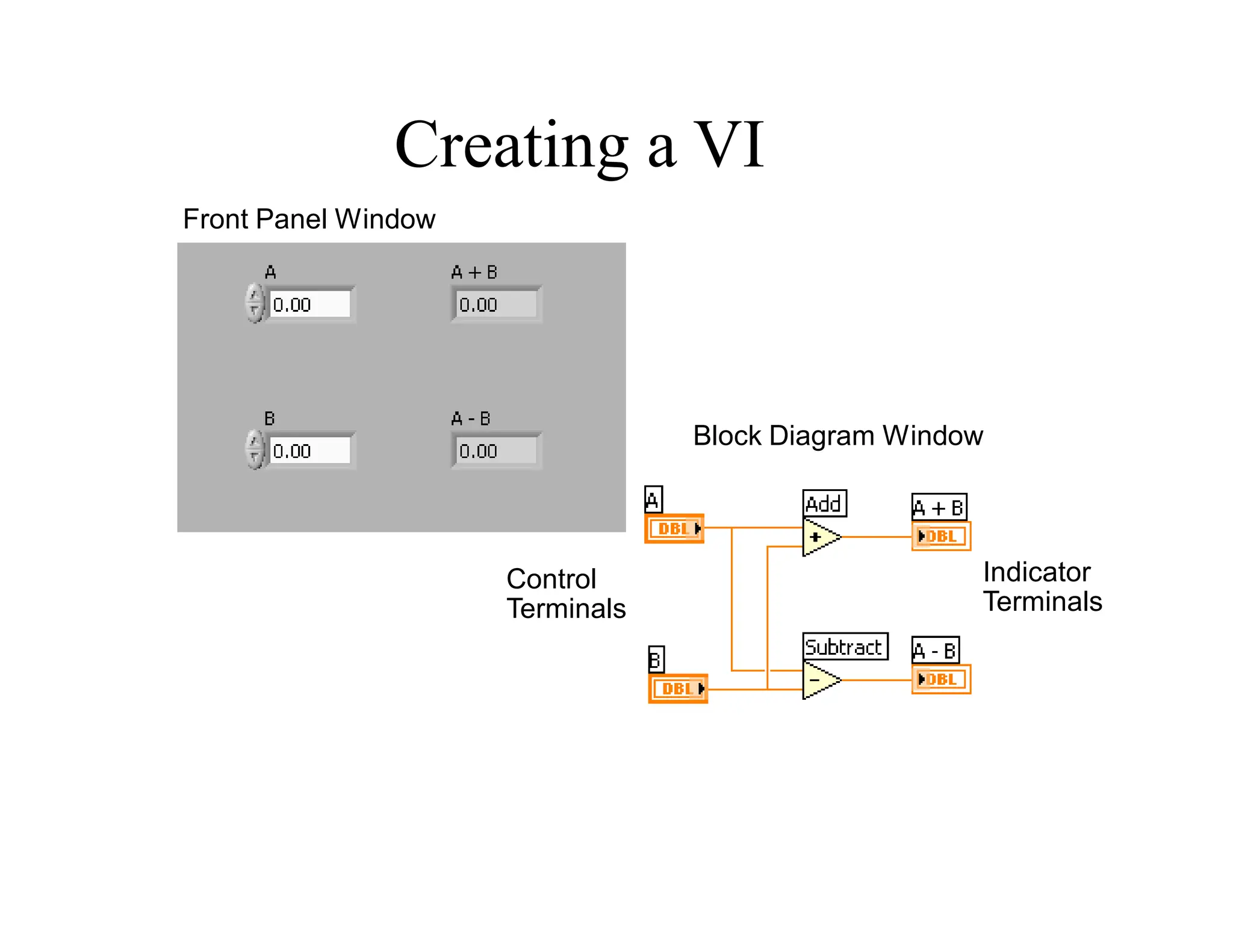


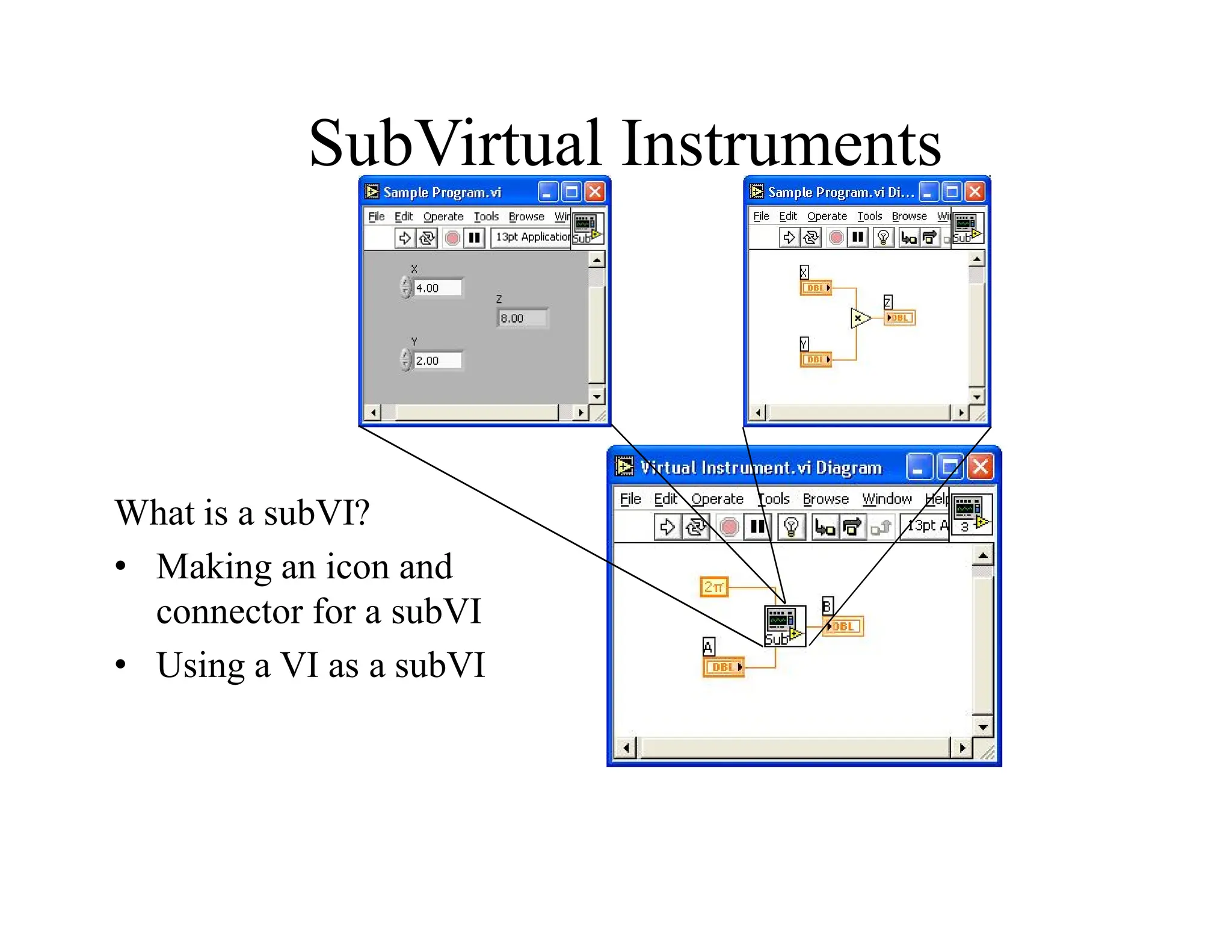


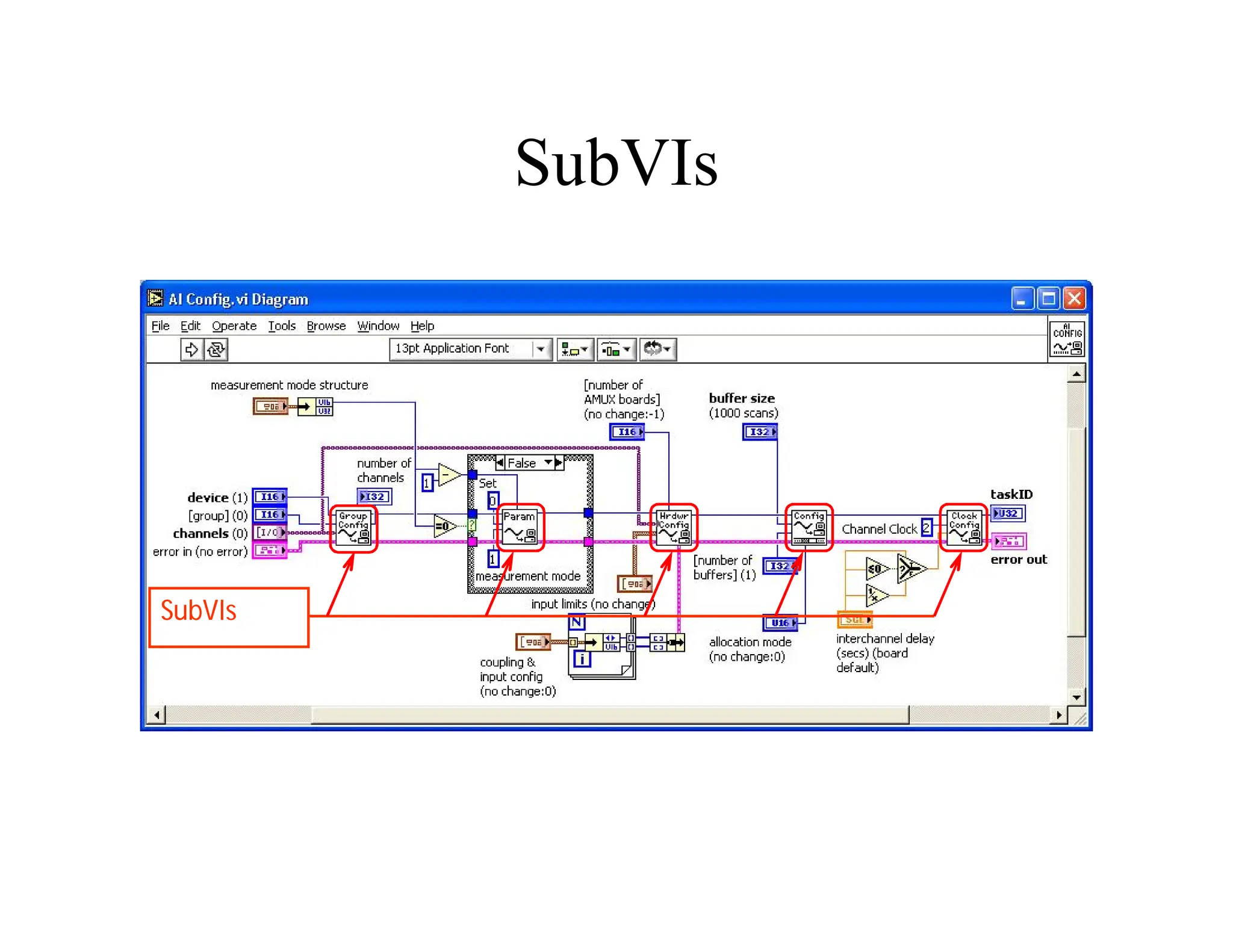


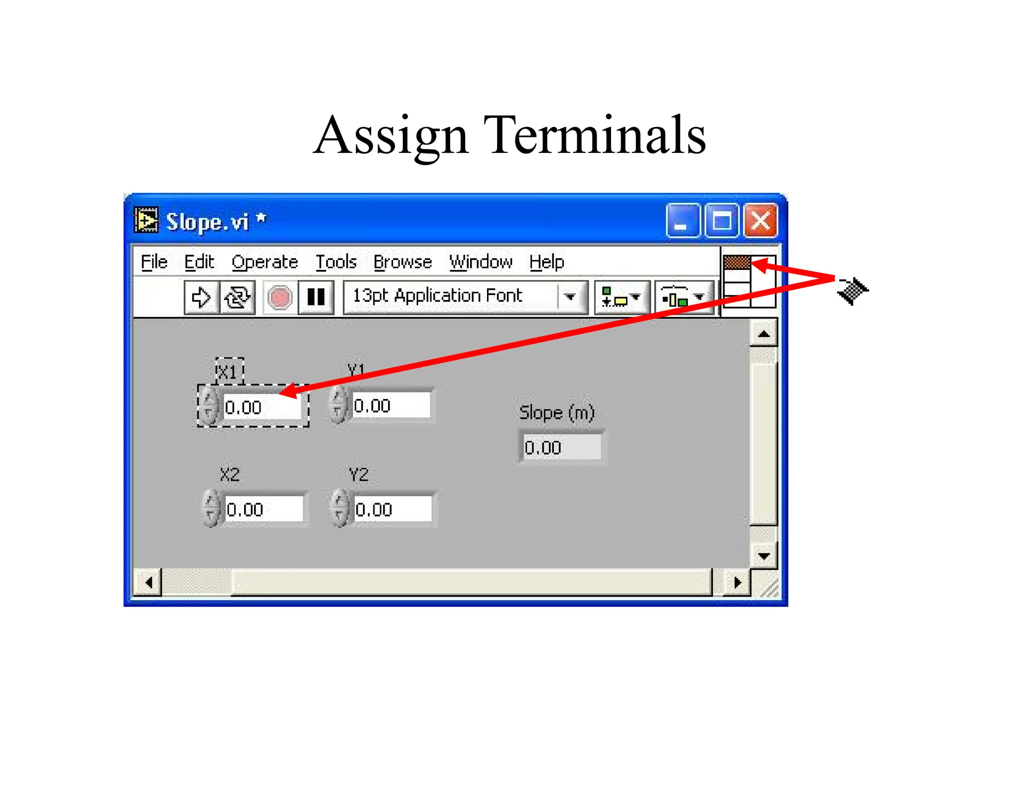


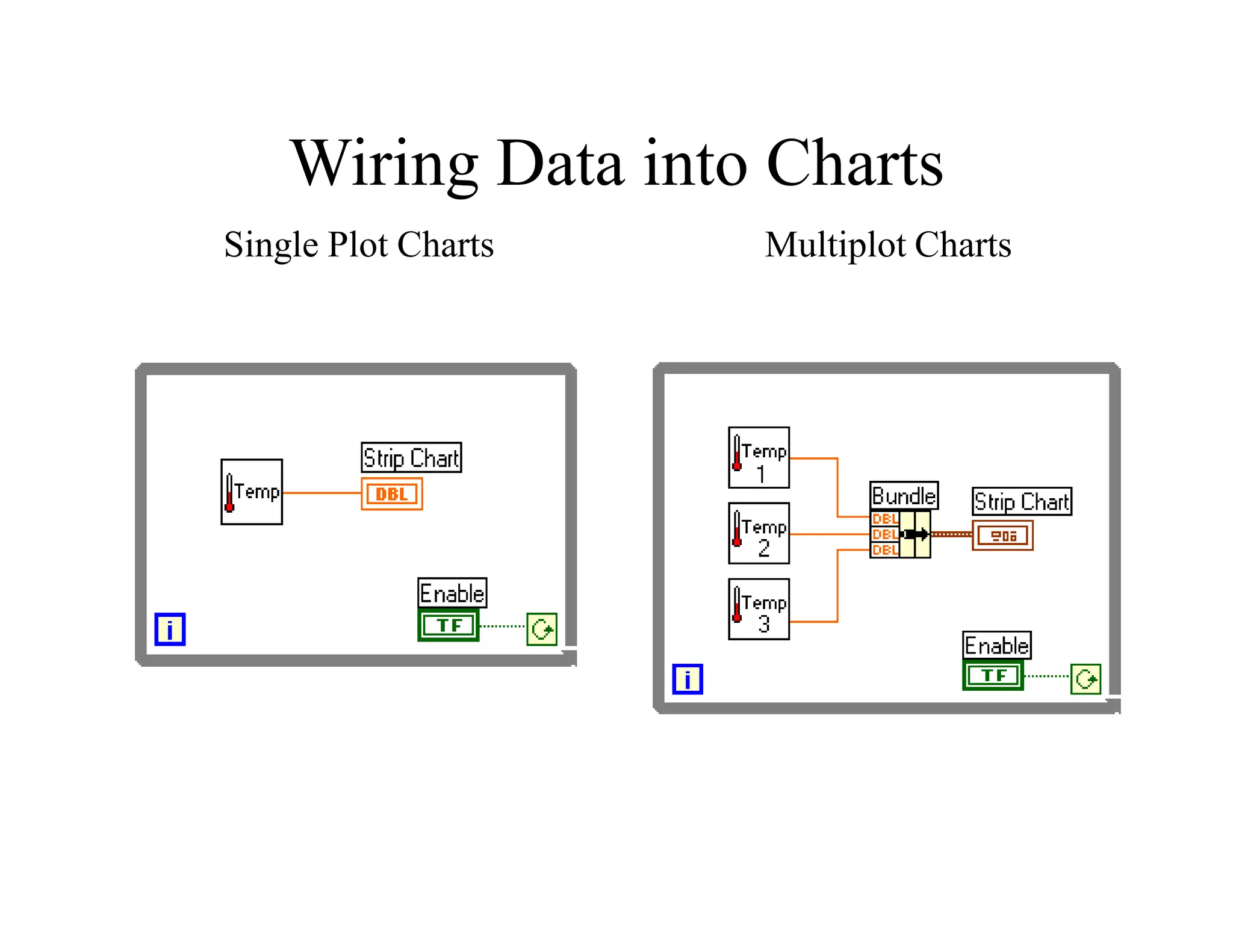
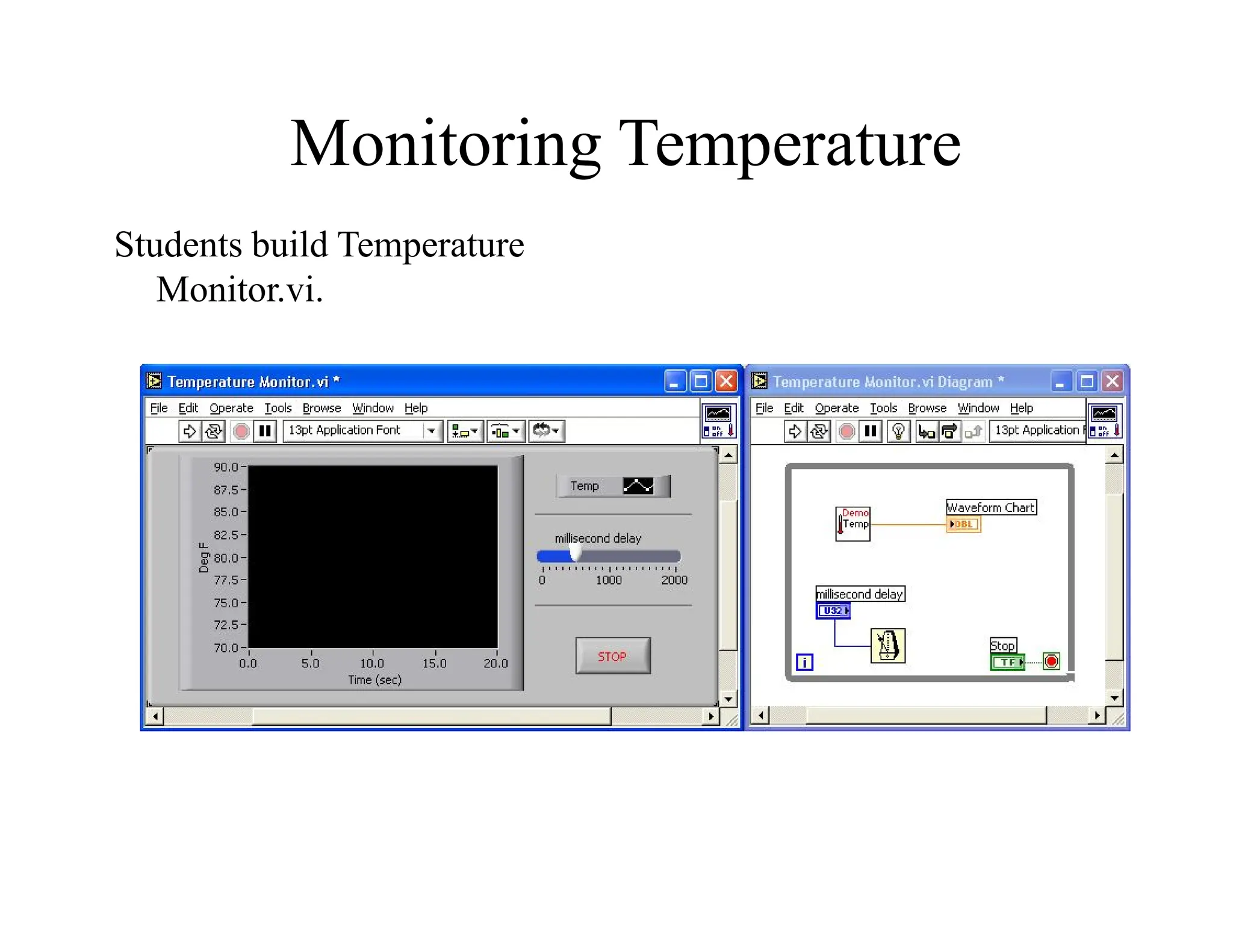

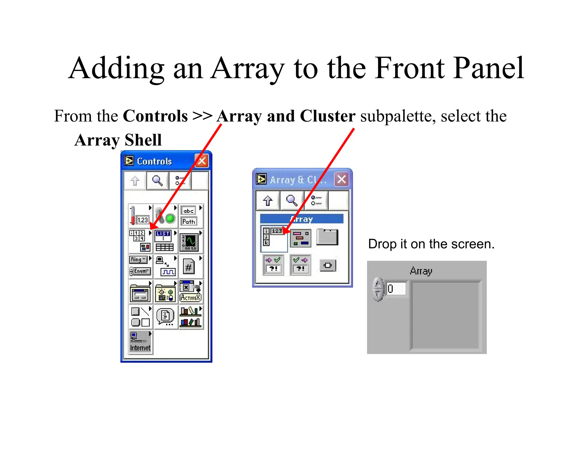


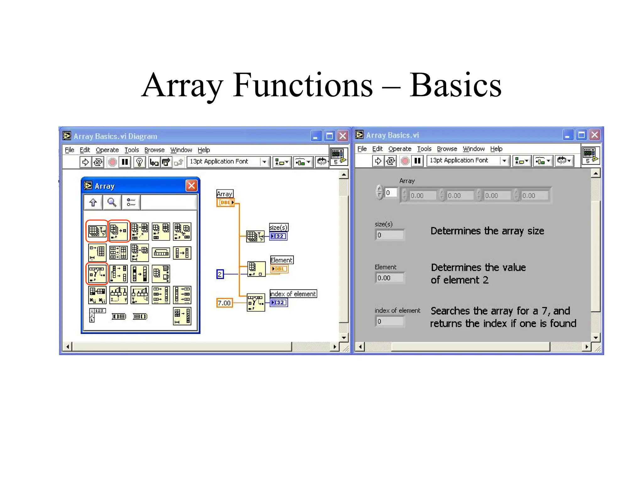

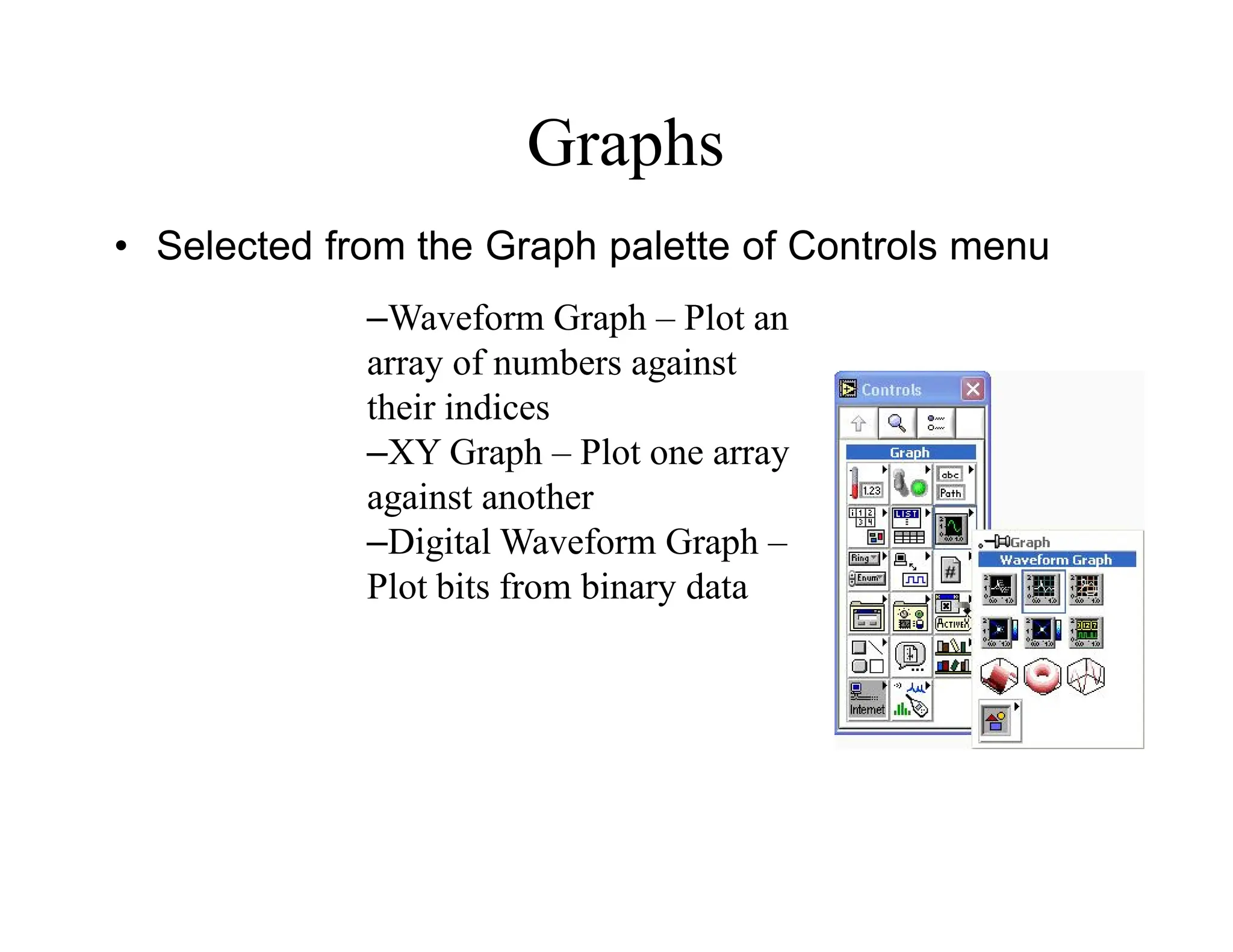

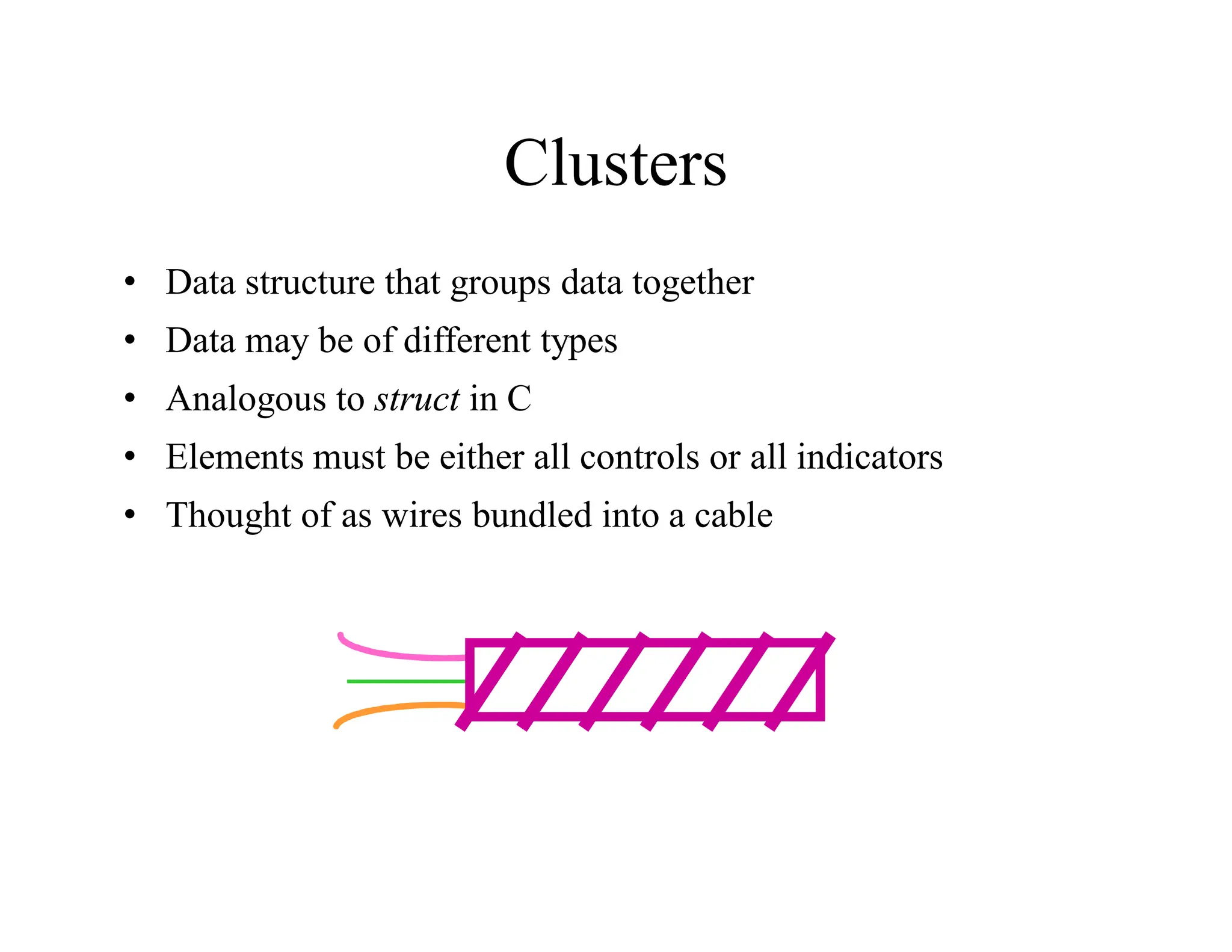


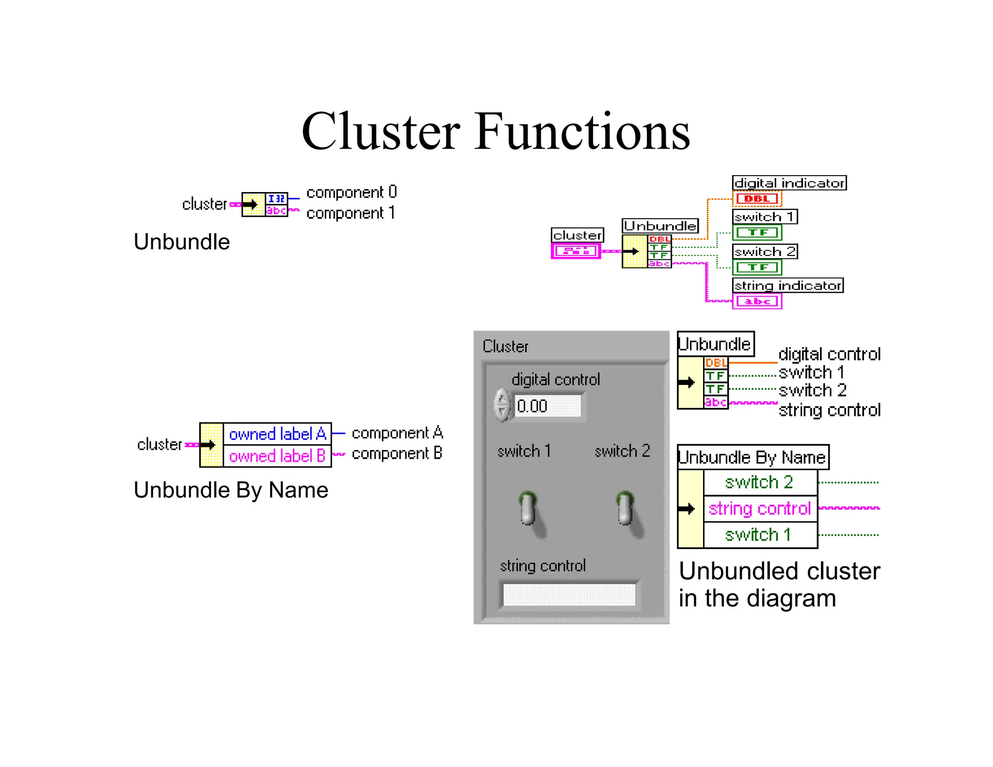
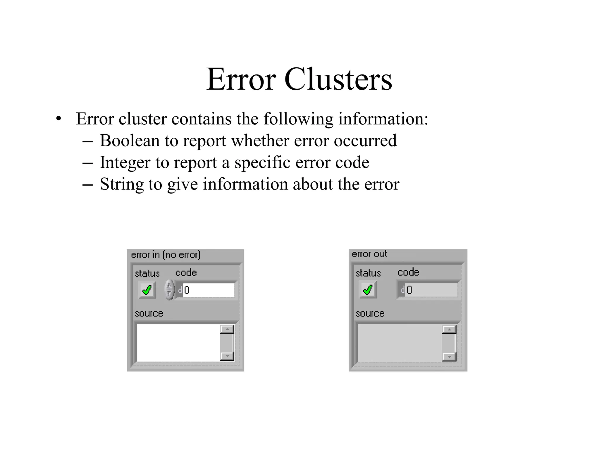

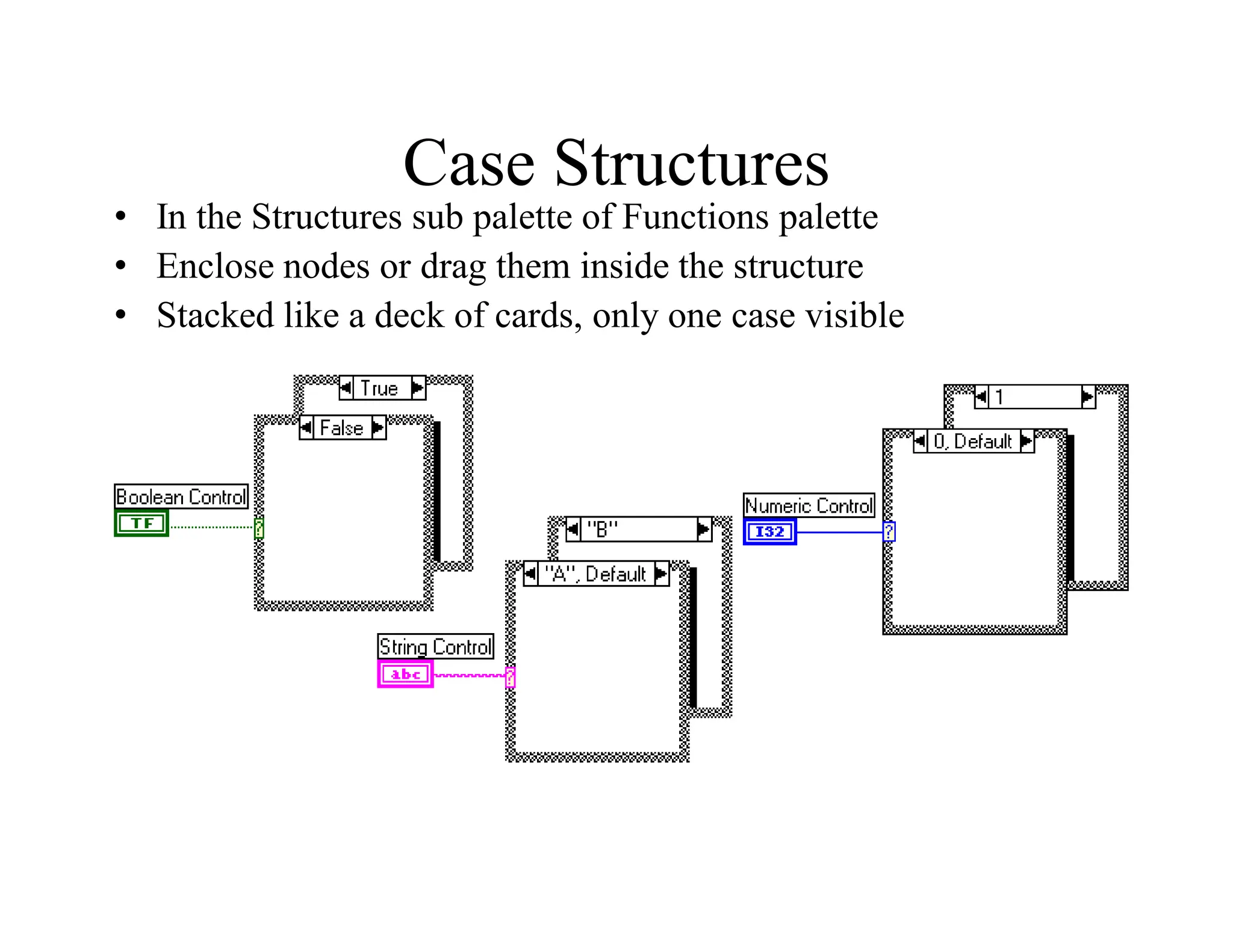

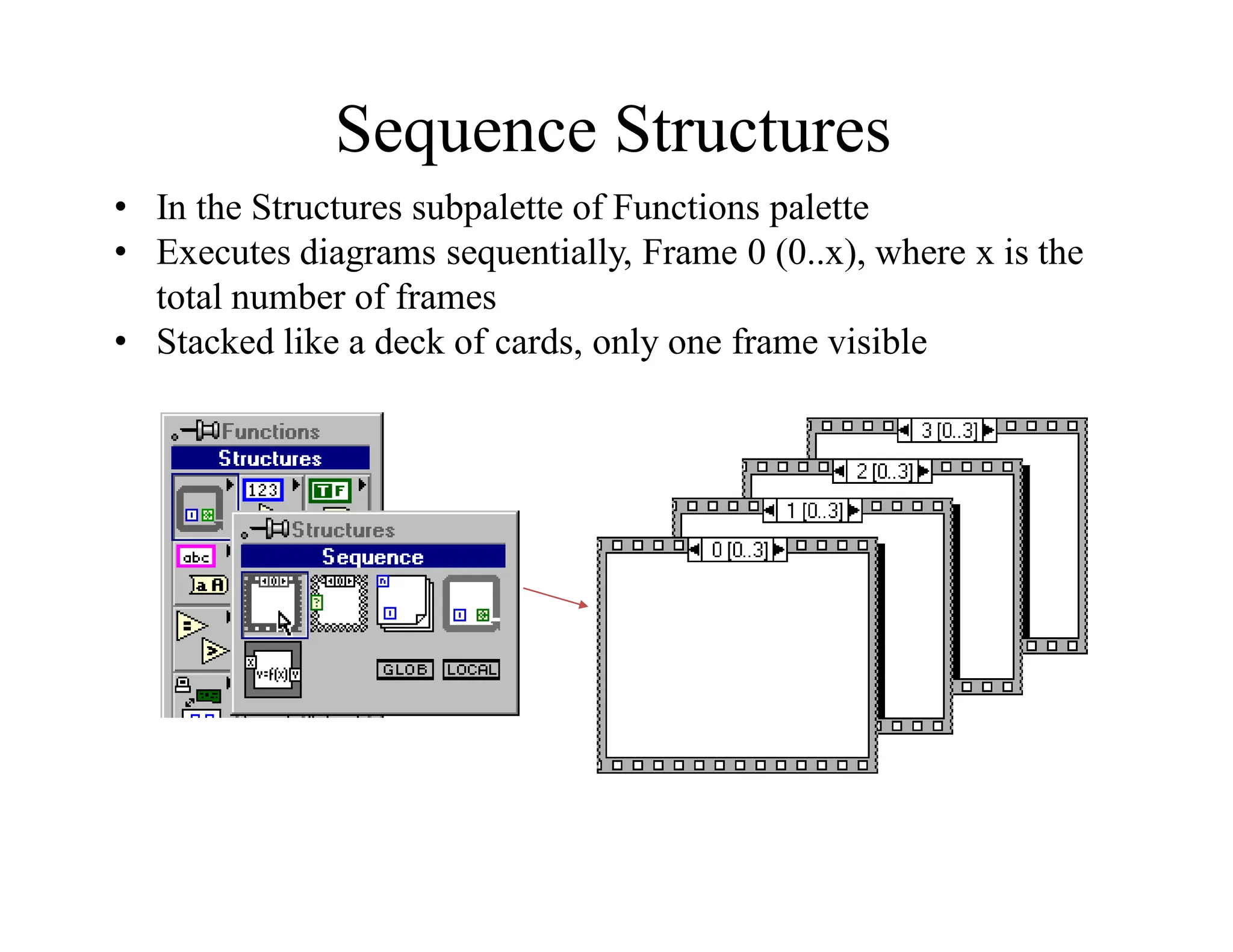

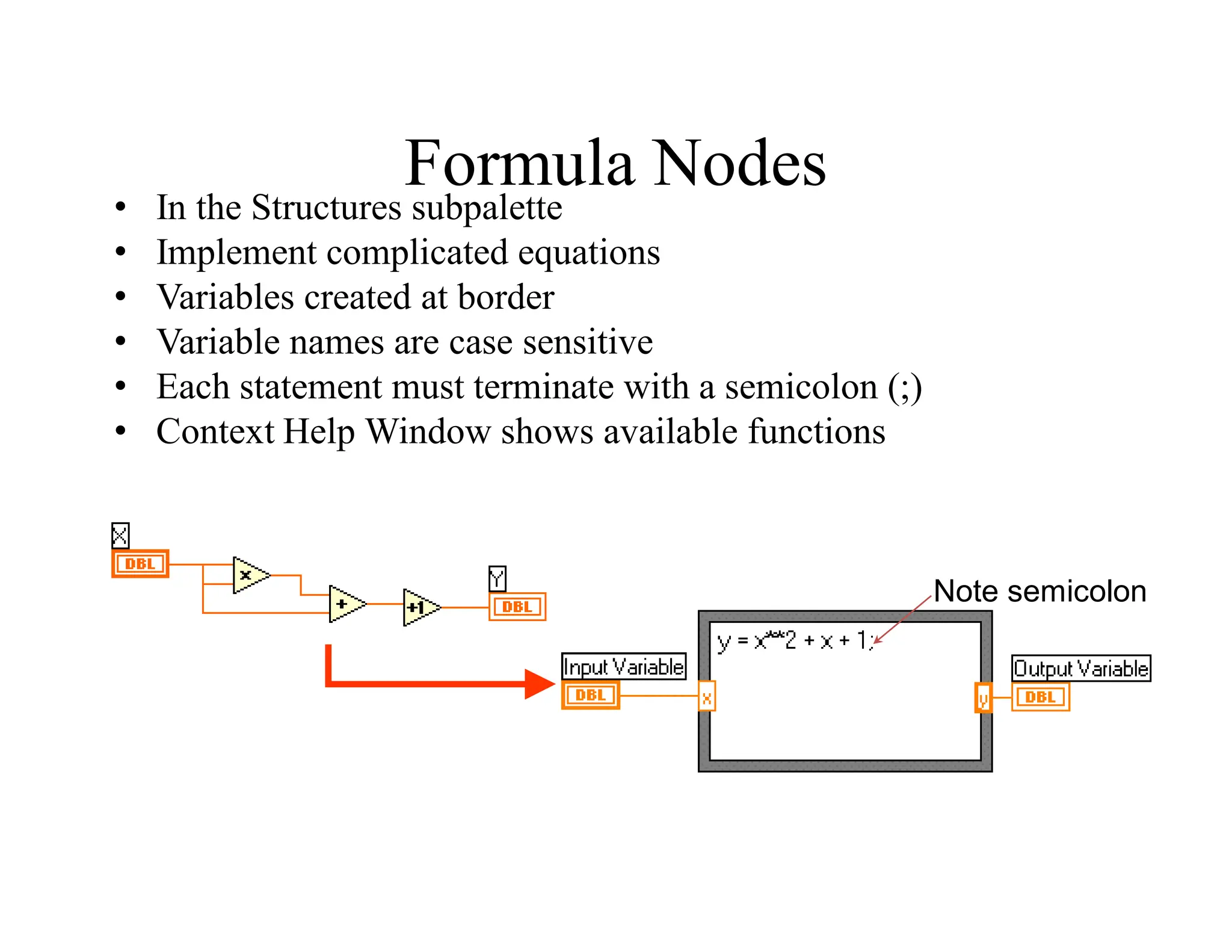

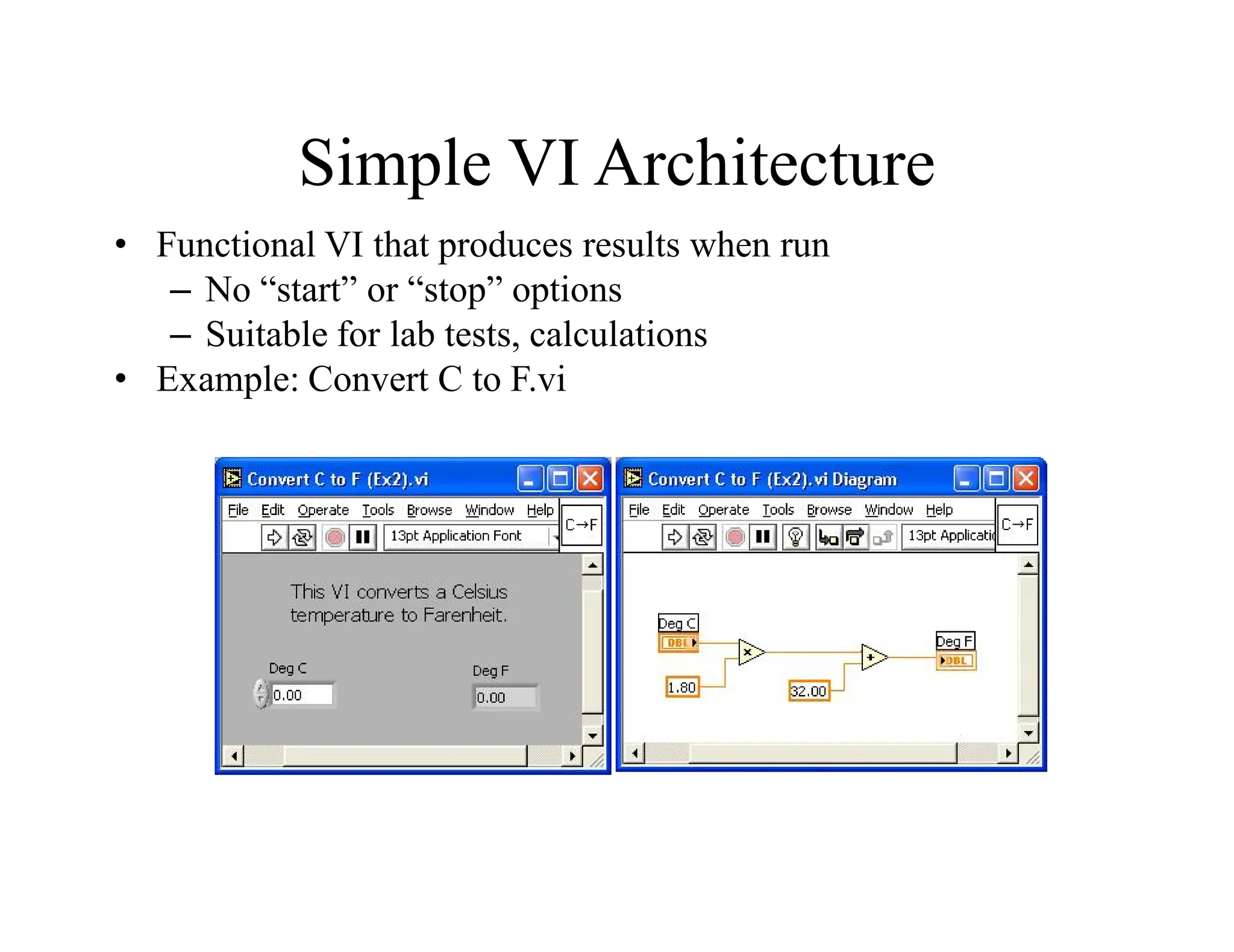
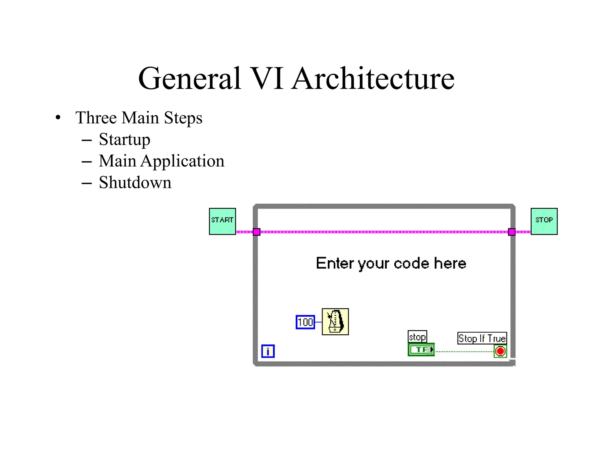
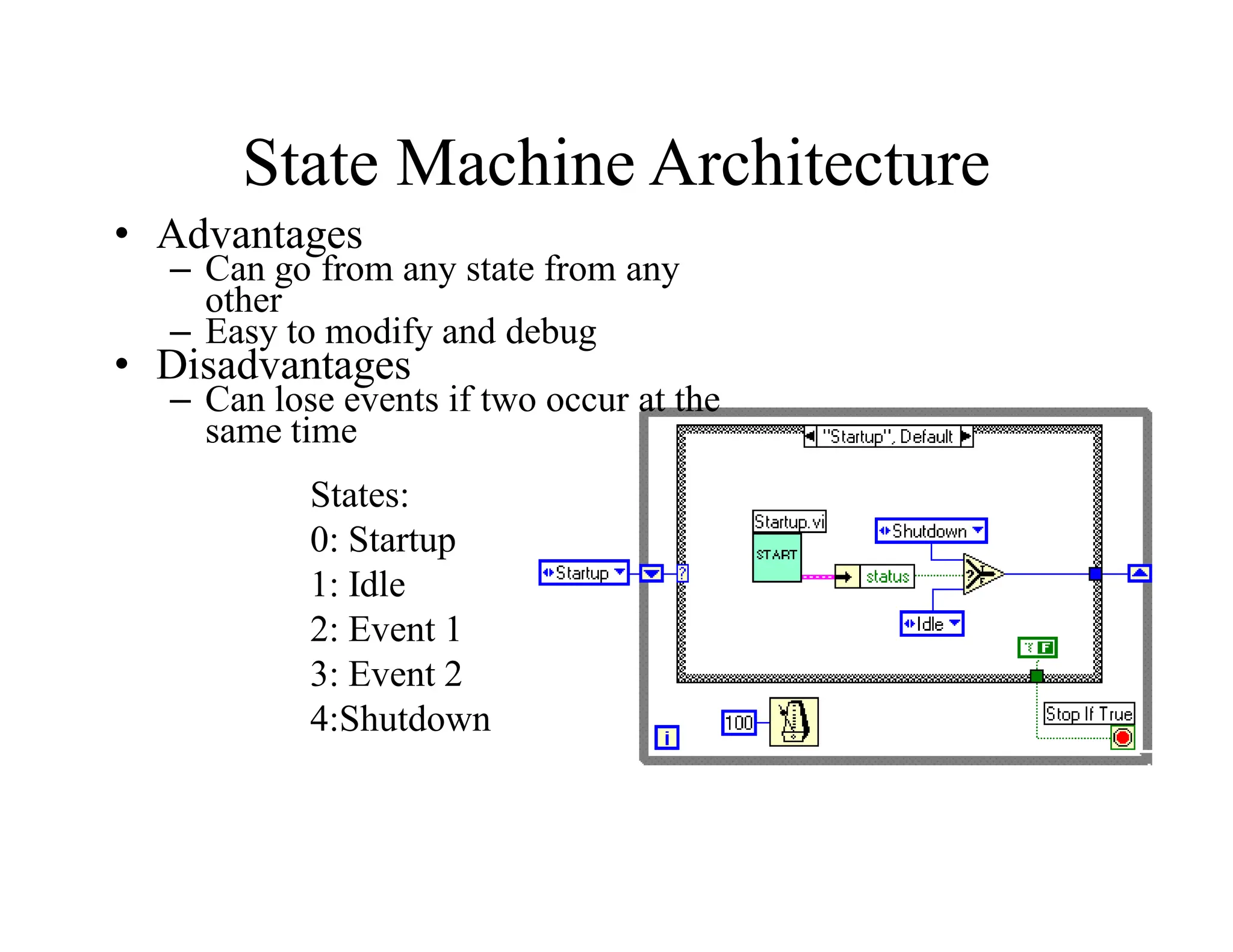


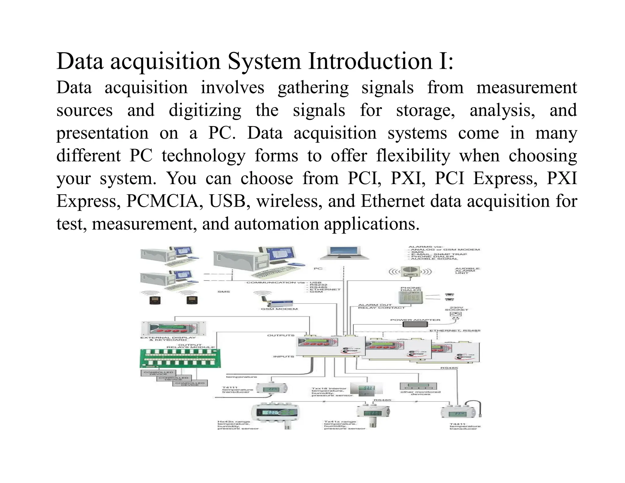


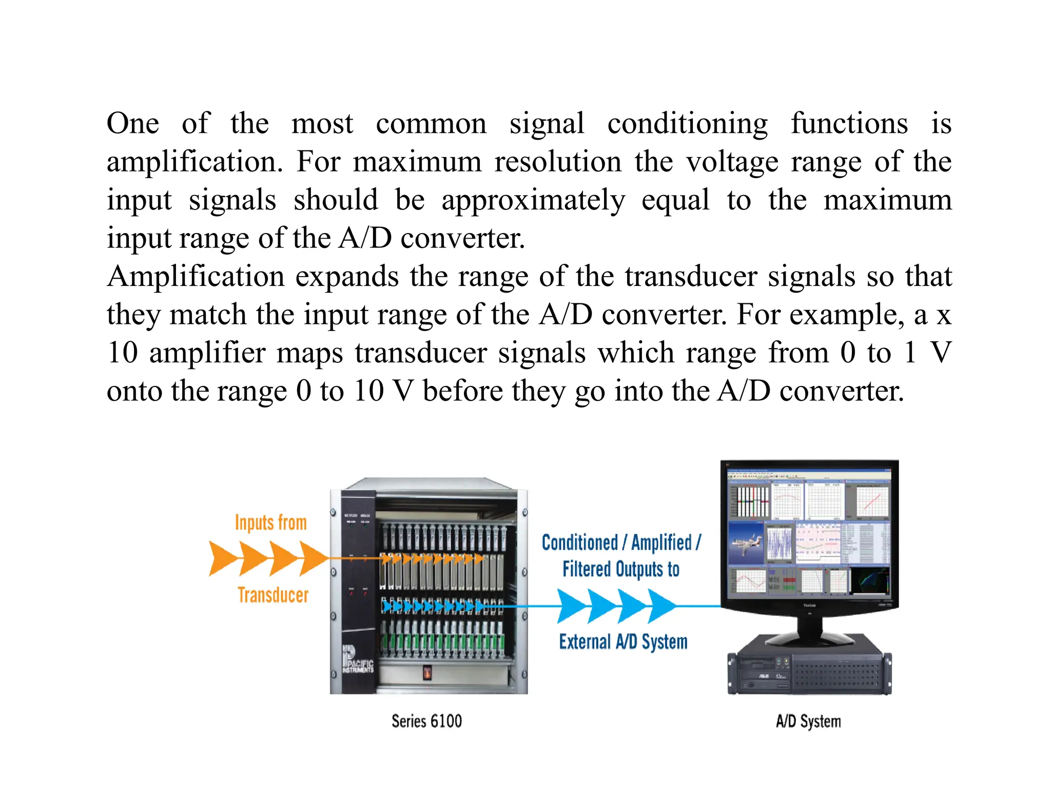
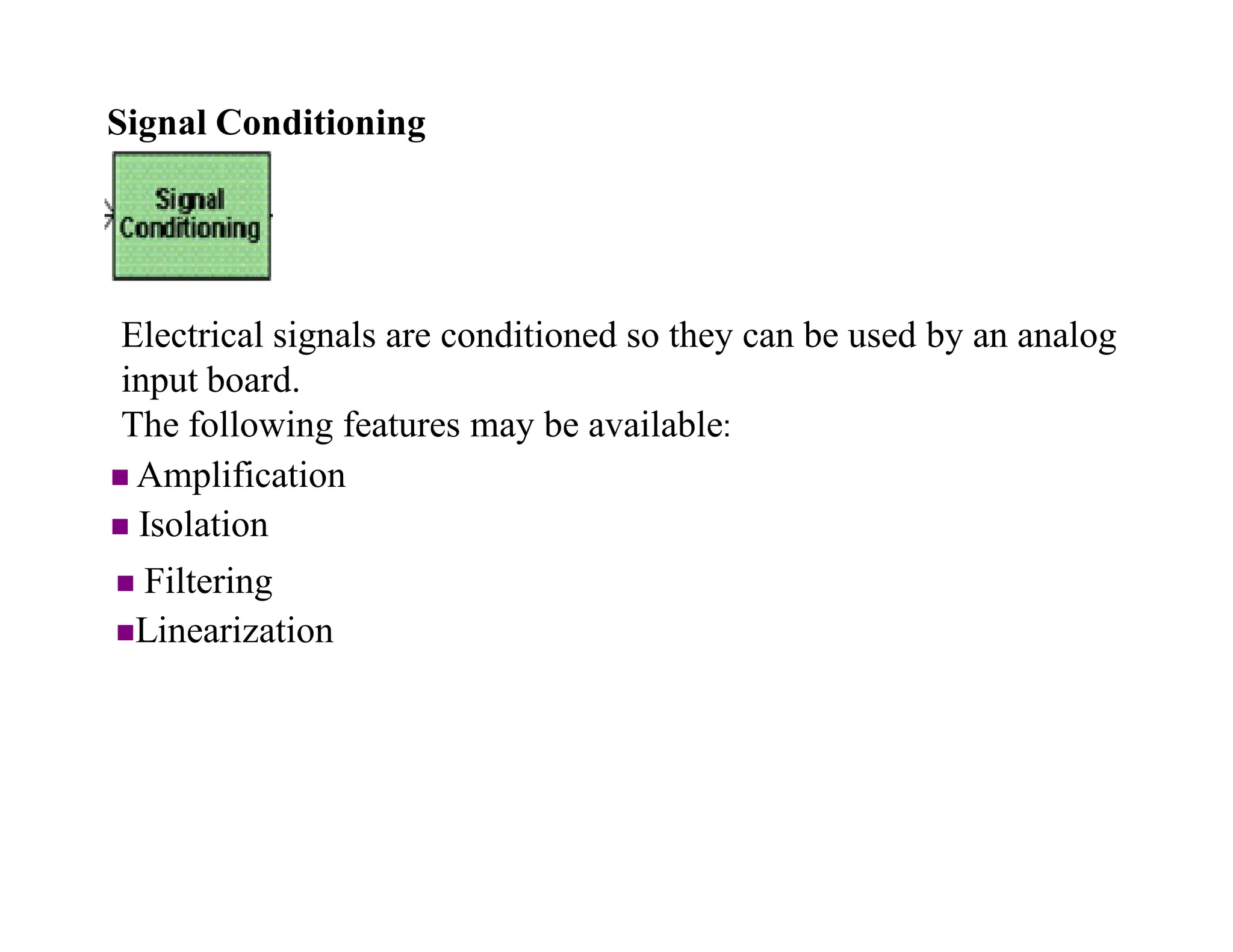


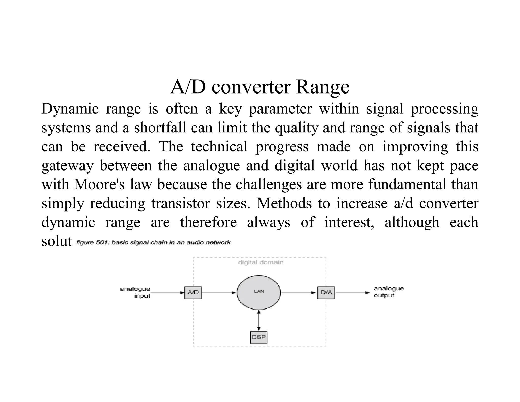
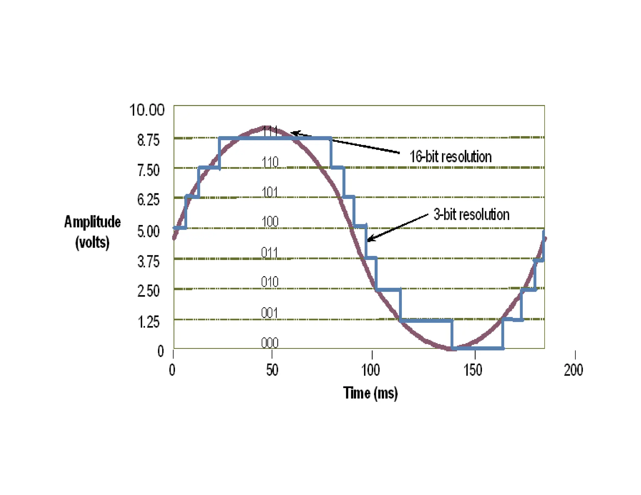


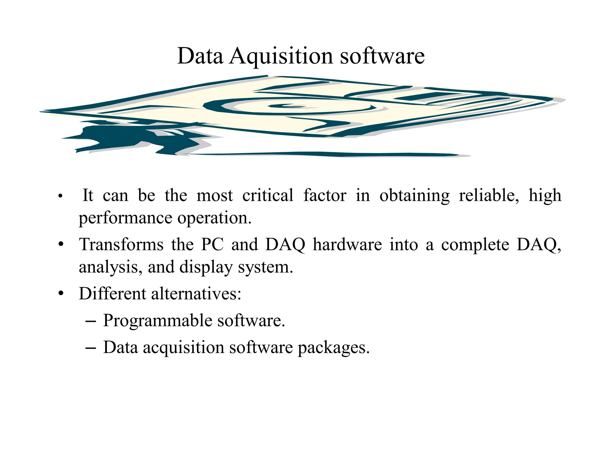
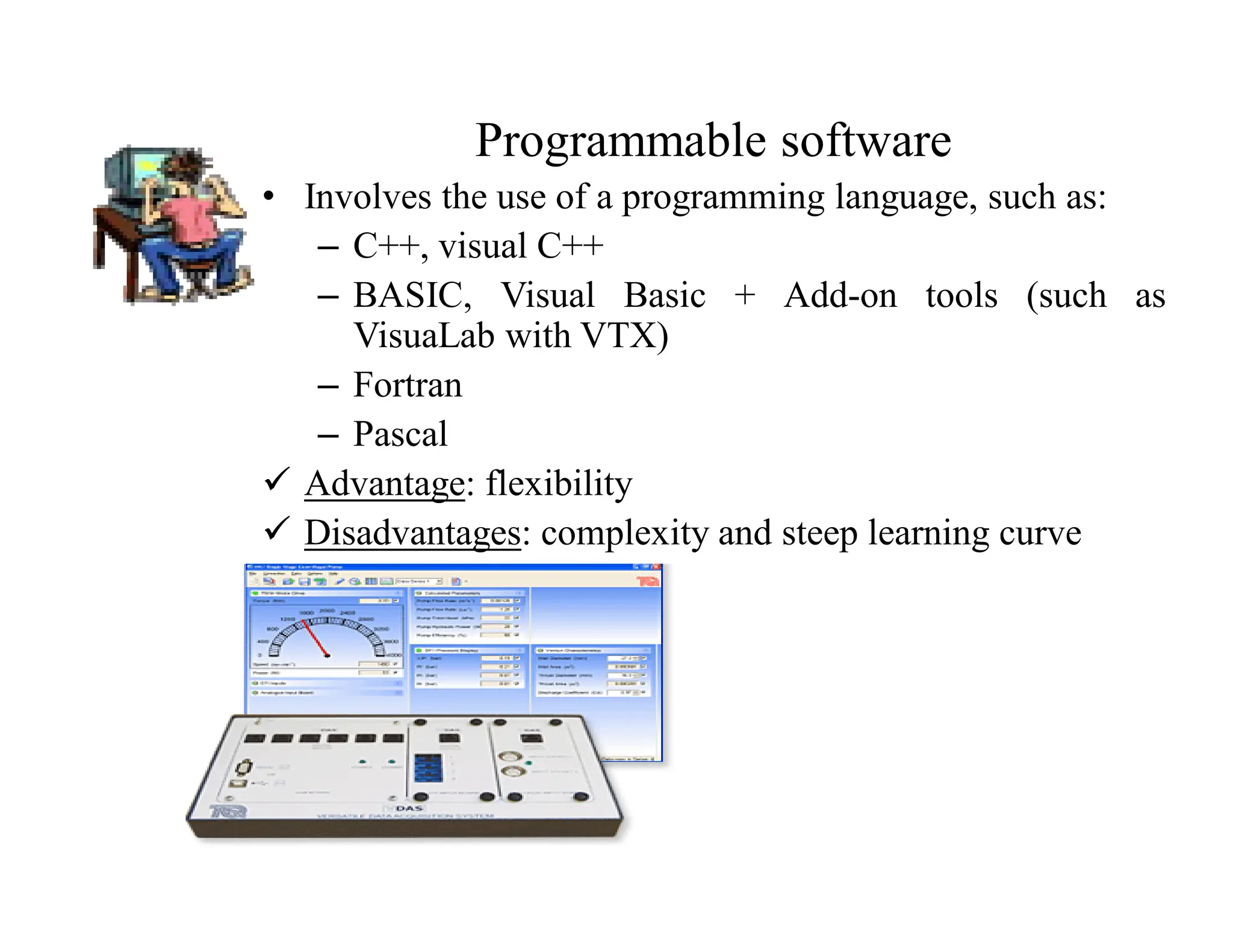
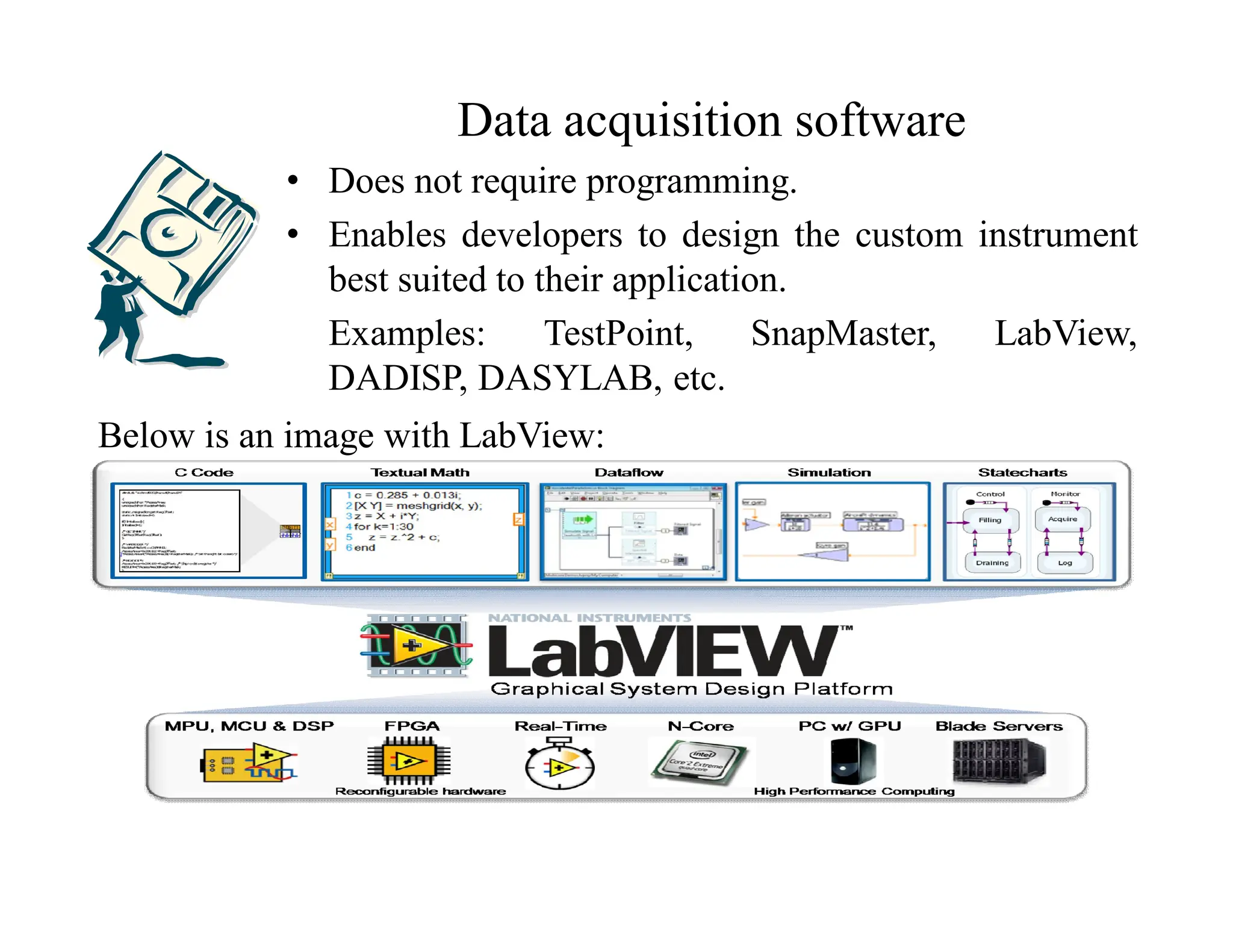
![Small Computer System Interface [SCSI]
Small Computer System Interface (SCSI), an ANSI
standard, is a parallel interface standard used by Apple
Macintosh computers, PCs, and many UNIX systems for
attaching peripheral devices to computers. SCSI interfaces
provide for faster data transmission rates than standard
serial and parallel ports. In addition, you can attach many
devices to a single SCSI port. There are many variations
of SCSI: SCSI-1, SCSI-2, SCSI-3 and the recently
approved standard Serial Attached SCSI (SAS).
SCSI-1 : SCSI-1 is the original SCSI and it is obsolet so
far. Basically, SCSI-1 uses an 8-bit bus, and supports data
rates of 4 MBps.](https://image.slidesharecdn.com/bei704-virtualinstrumentation-250502073717-4ebd7929/75/BEI704-virtual-instrumentation-For-E4-pdf-101-2048.jpg)


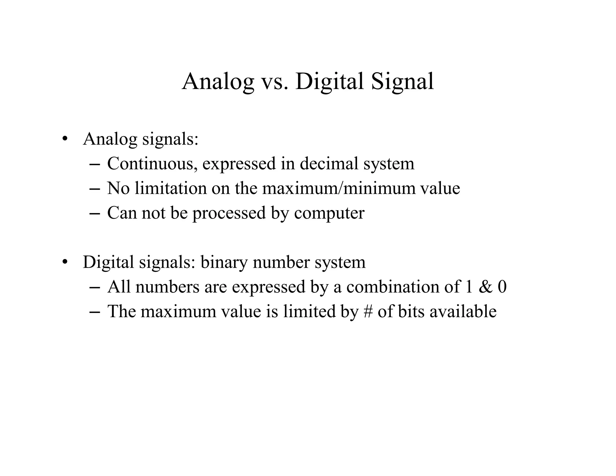
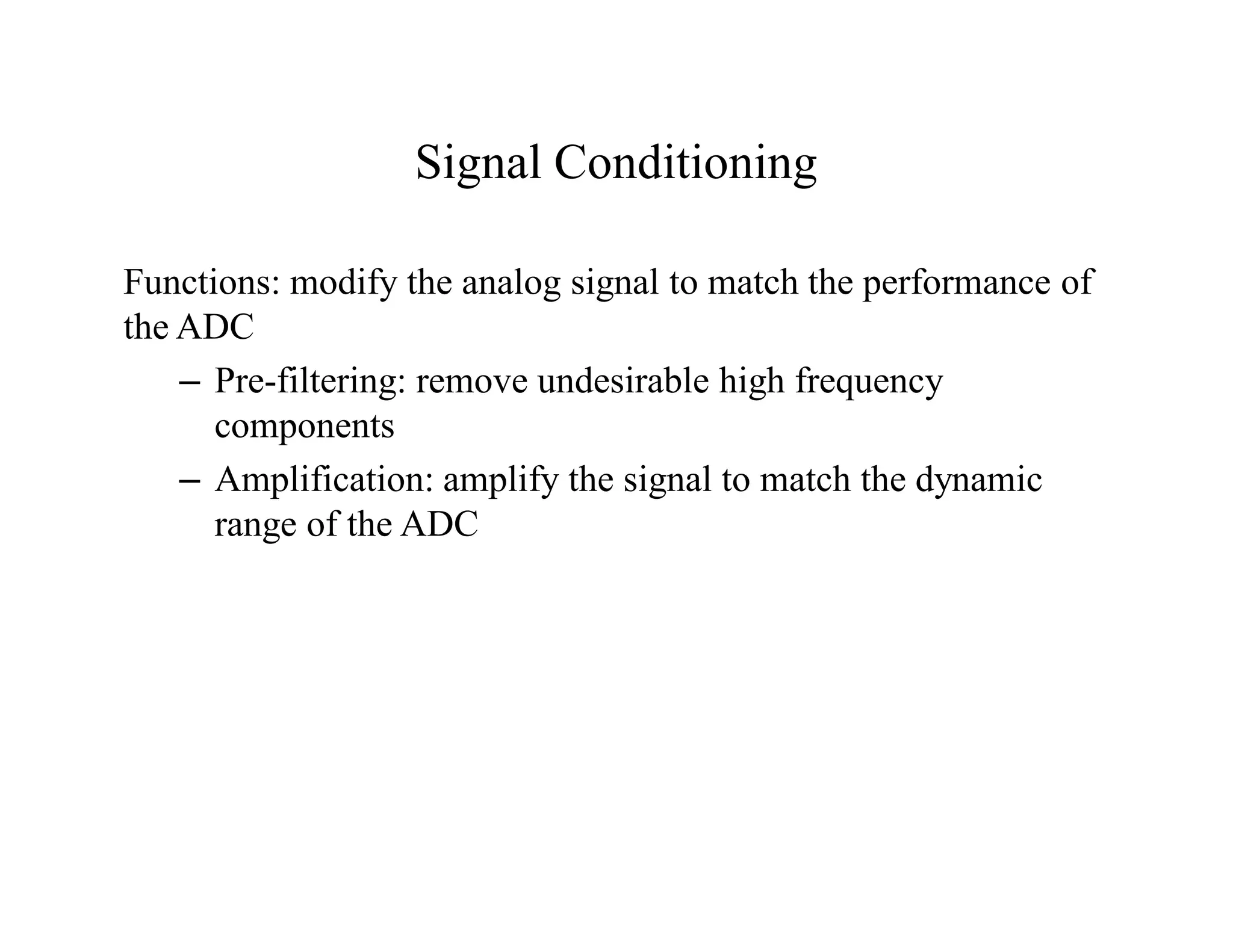

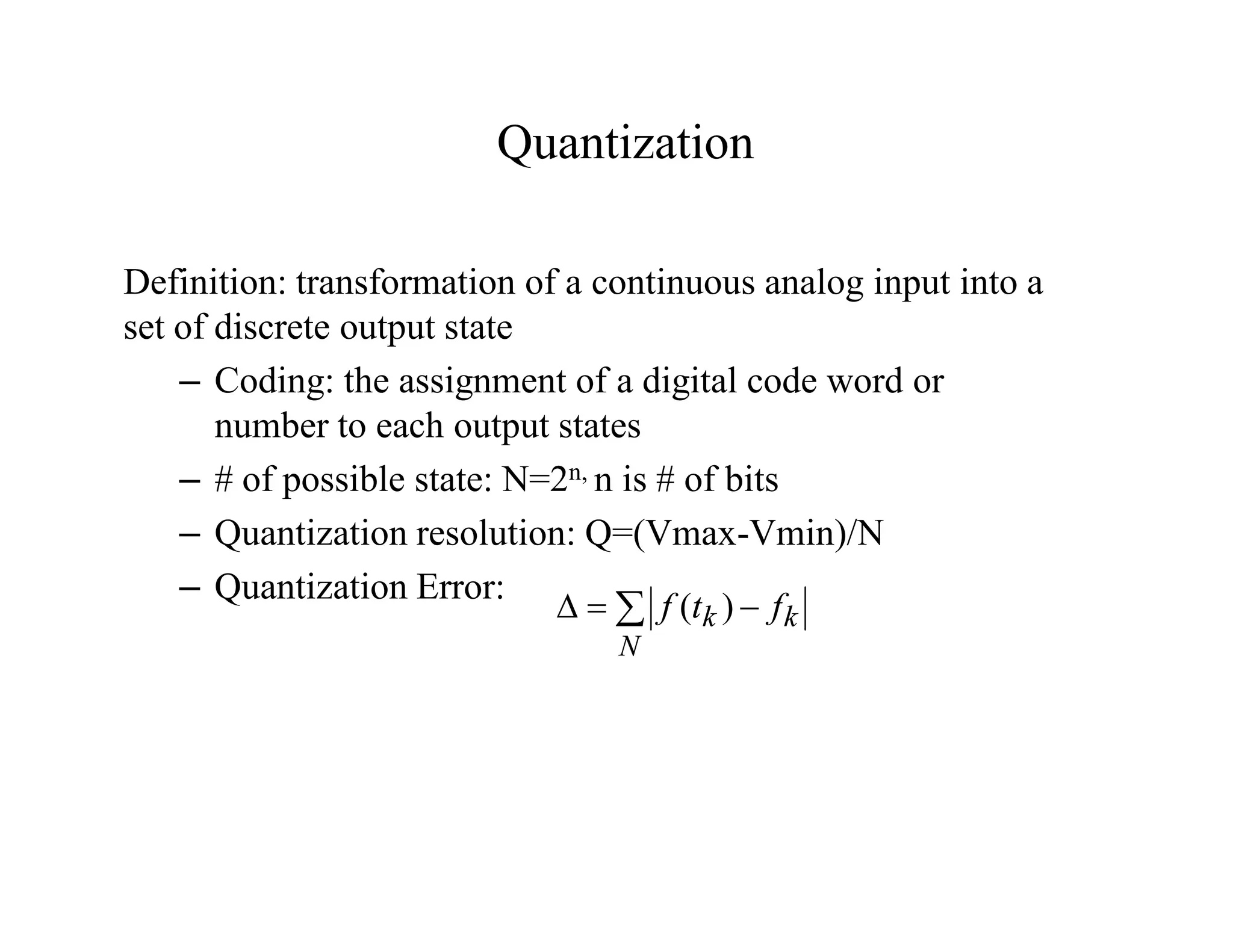


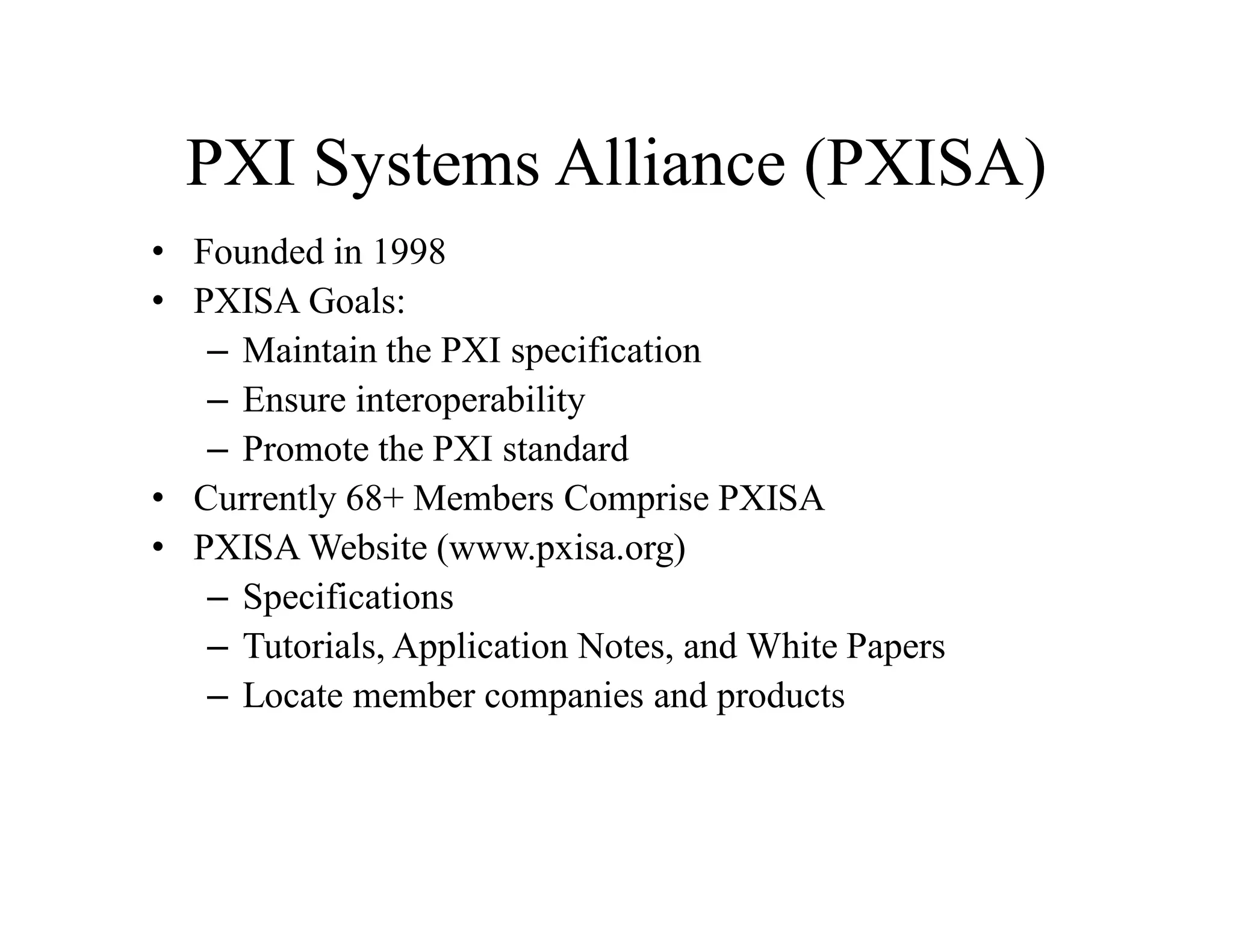

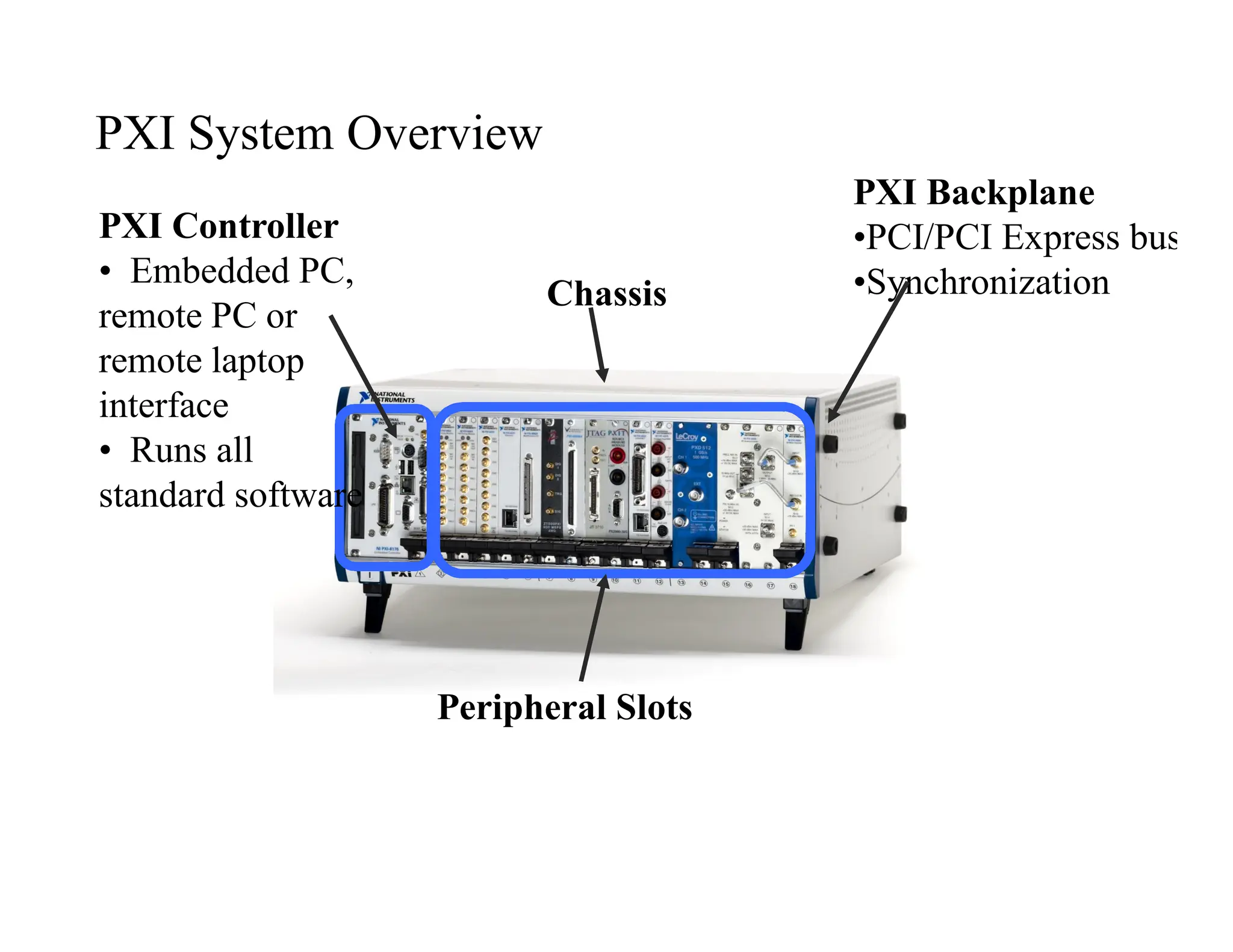


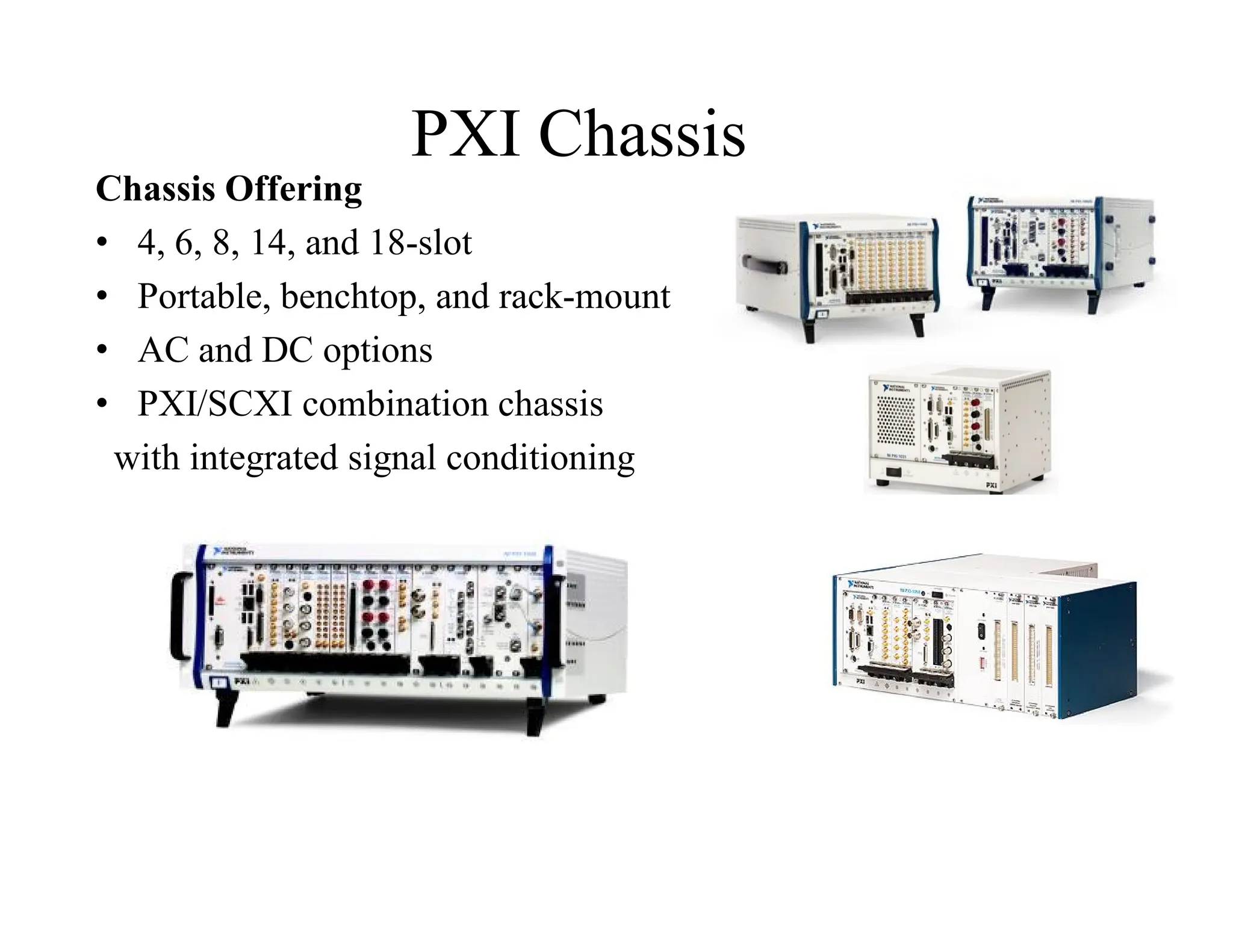


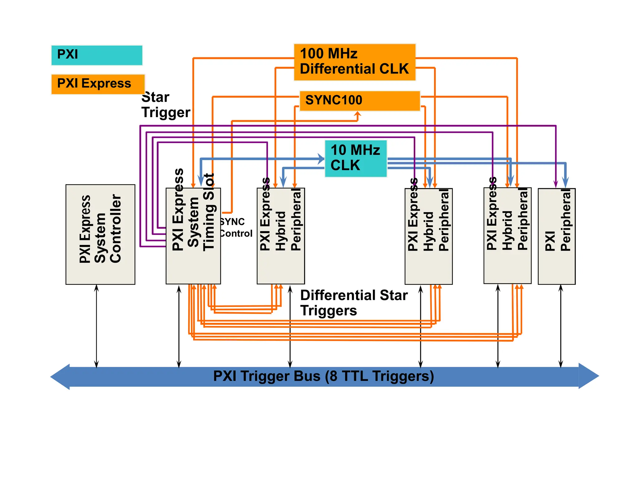
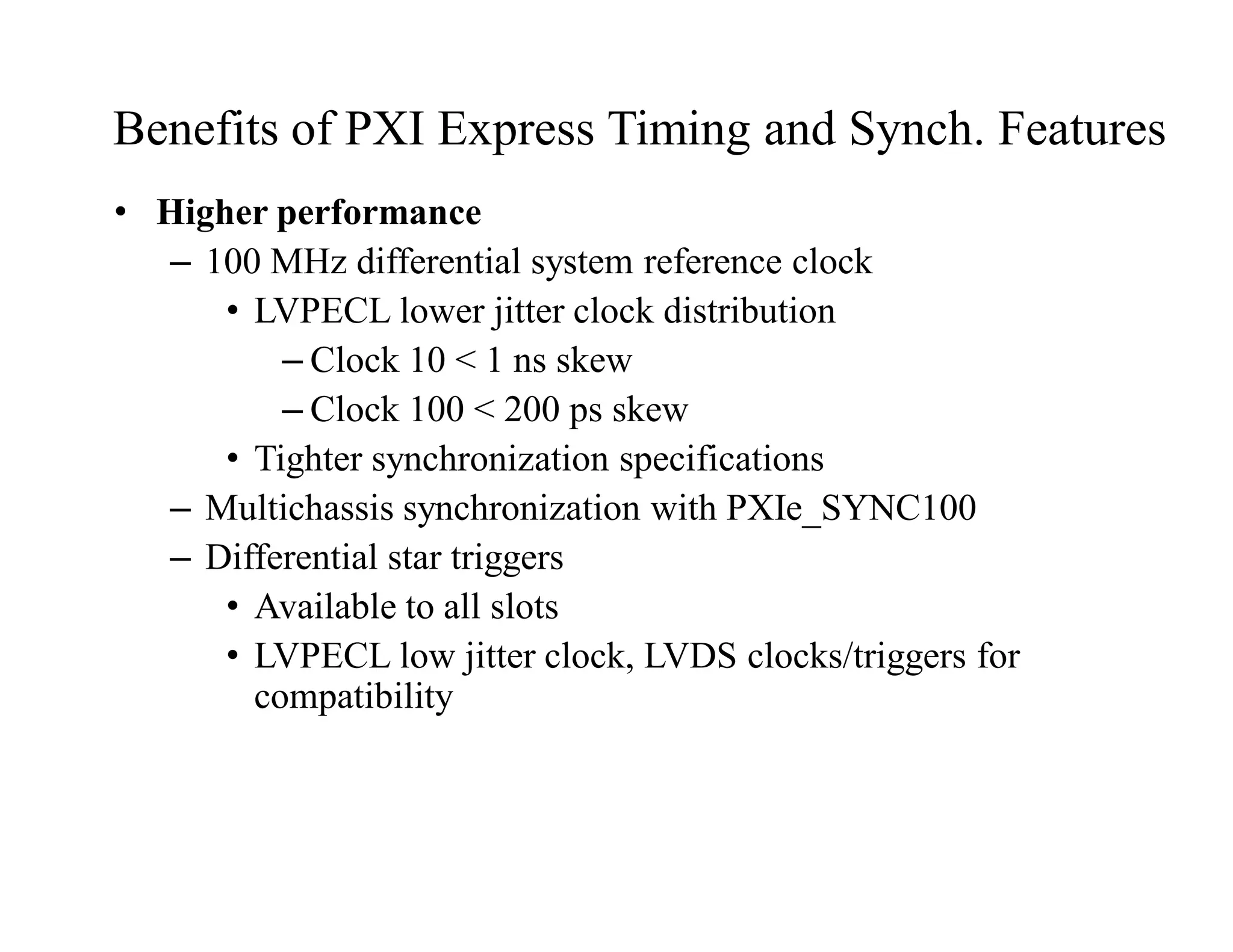
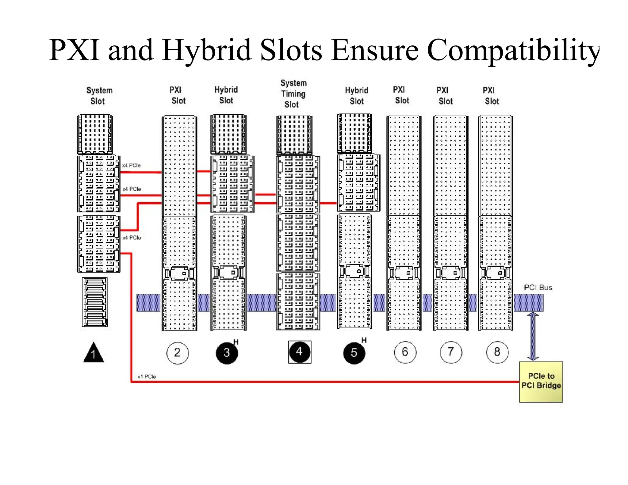

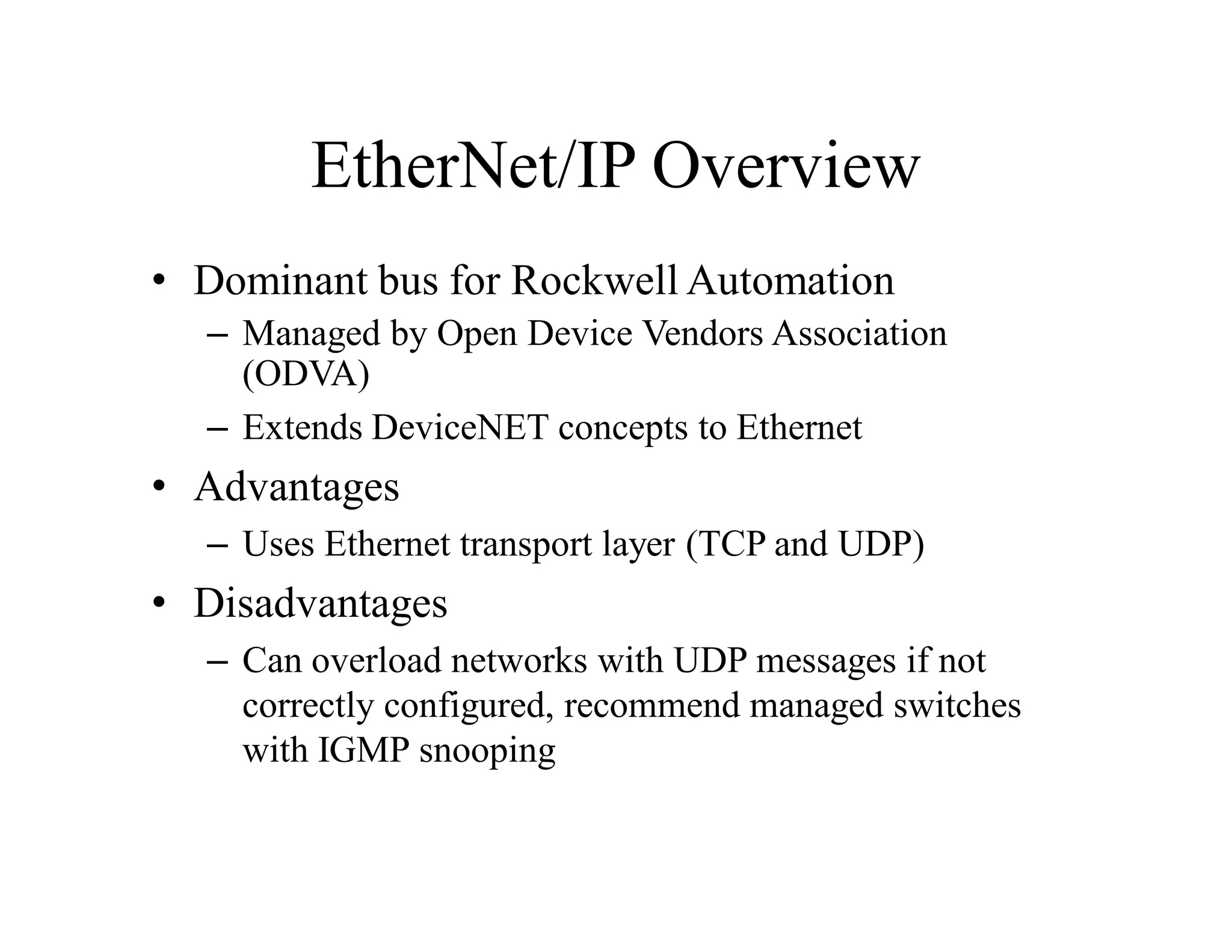
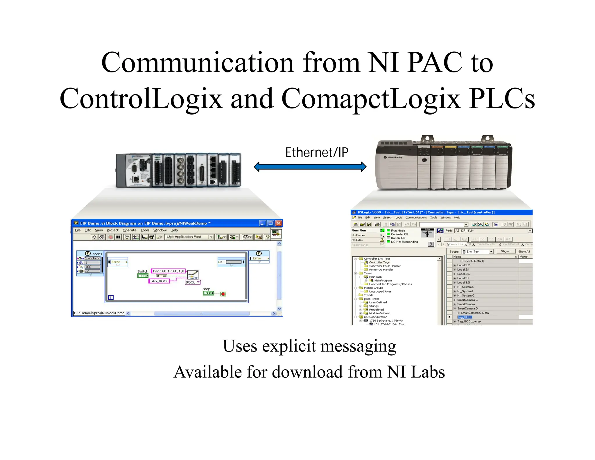


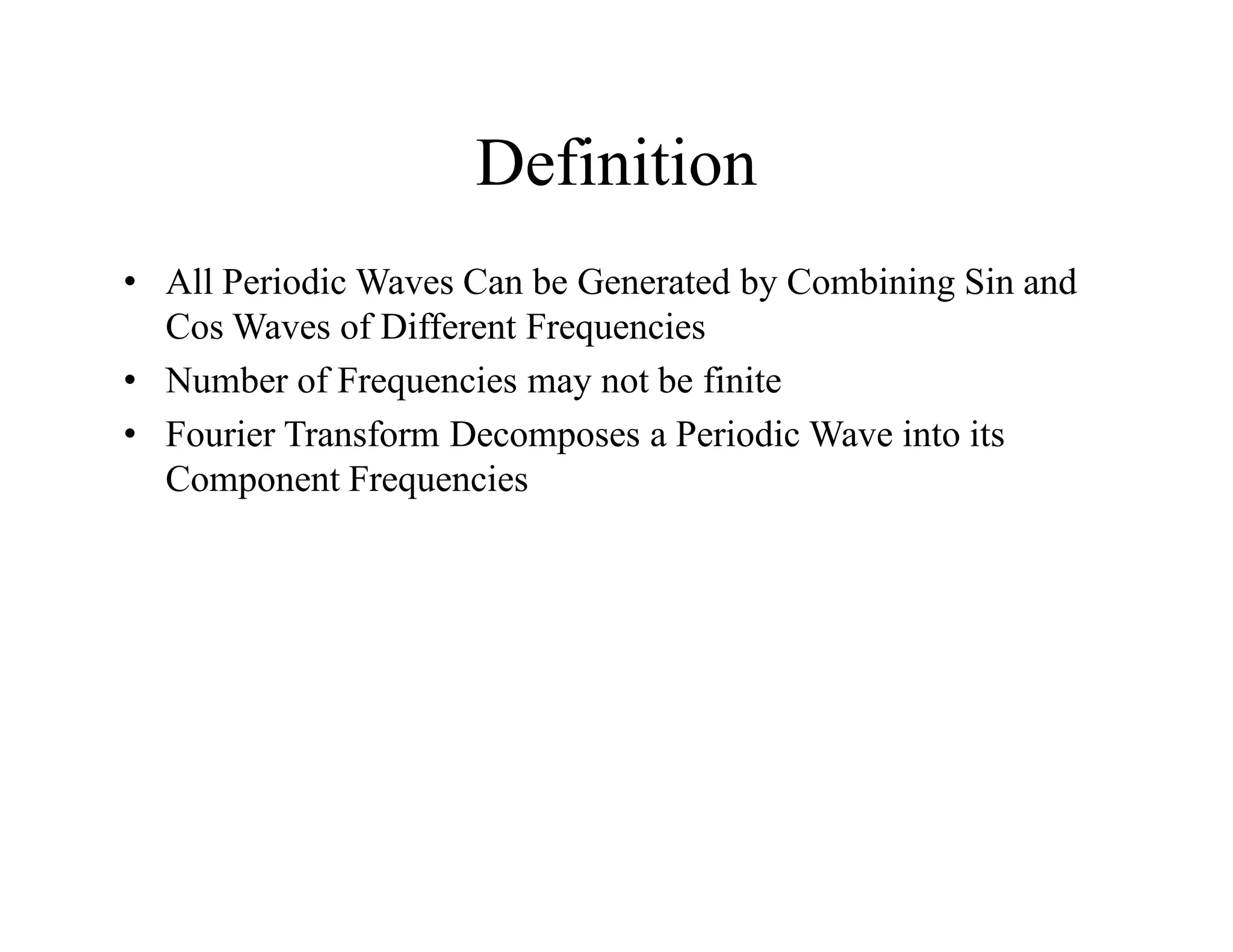


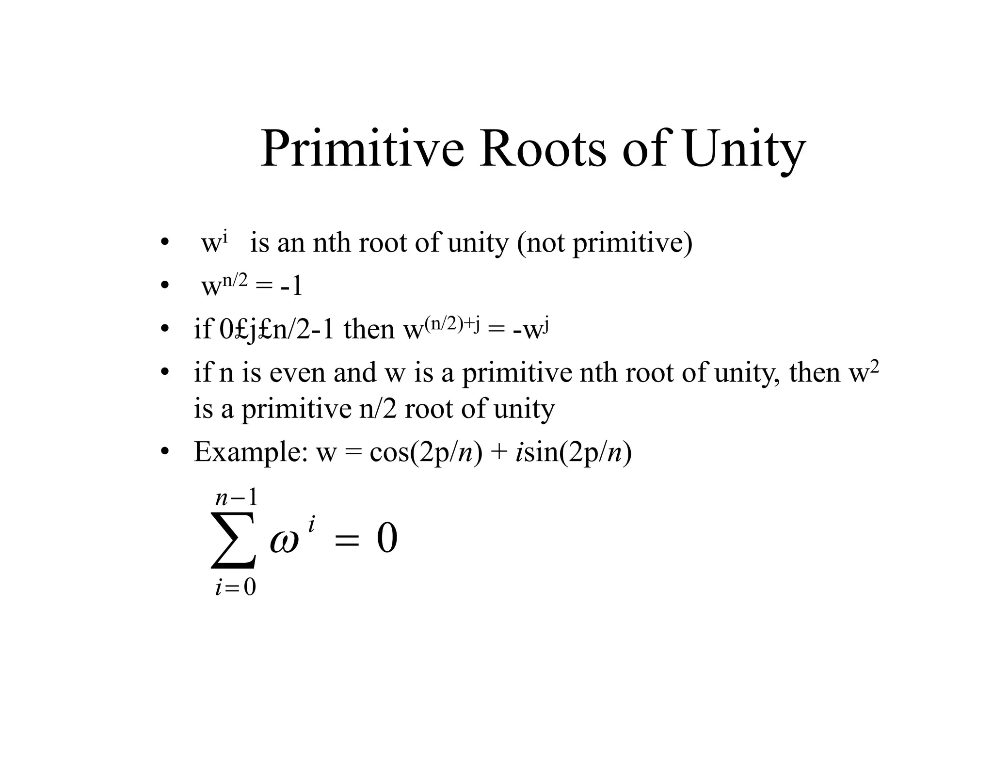


![Windowing in Frequency Domain
• Windowed frequency response
• The windowed version is smeared version of desired response
• If w[n]=1 for all n, then W(ejw) is pulse train with 2 period
w
w
w
d
e
W
e
H
2
1
e
H j
j
d
j](https://image.slidesharecdn.com/bei704-virtualinstrumentation-250502073717-4ebd7929/75/BEI704-virtual-instrumentation-For-E4-pdf-144-2048.jpg)