Downloaded 14 times


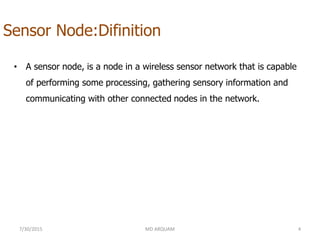


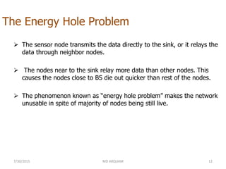


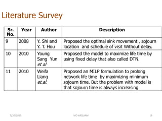

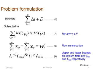


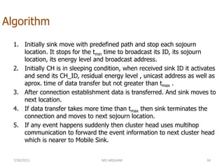
![Comparison of DCRP v/s MILP
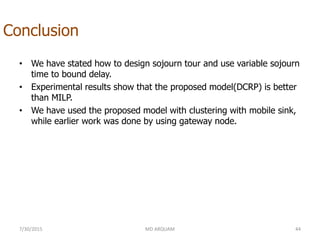
Name of Parameter DCRP MILP
Average Throughput[kbps] 197.55 162.03
Average Delay 89.598 287.293
Packet Delivery Ratio 0.9999 0.8084
Total Energy Consumption 204.125 187.049
Avg Energy Consumption 5.1475 6.44996
Overall Residual Energy 1298.47 1262.95
Avg Residual Energy 45.457 43.55
7/30/2015 MD ARQUAM 38](https://image.slidesharecdn.com/8480a6fd-7758-4fbd-8630-38db4752815c-150730134908-lva1-app6892/85/Arquam_reportfinal-37-320.jpg)
![References
[1] Gupta, C. P., and Arun Kumar. "Wireless Sensor Networks: A
Review."International Journal of Sensors Wireless Communications and
Control 3.1 (2013): 25-36.
[2] Akyildiz, Ian F., et al. "Wireless sensor networks: a survey." Computer
networks 38.4 (2002): 393-422.
[3] Ganesan et.al., Networking issues in wireless sensor networks, J. Parallel
Distrib. Comput. 64 (2004) 799–814.
[4] Ahmed, Nadeem, Salil S. Kanhere, and Sanjay Jha. "The holes problem in
wireless sensor networks: a survey." ACM SIGMOBILE Mobile Computing and
Communications Review 9.2 (2005): 4-18.
[5] Horst F. Wedde and Muddassar Farooq. “A Comprehensive review of nature
inspired routing algorithms for fixed telecommunication networks” Journal of
Systems Architecture, Vol. 52, 2006, pp. 461- 484.
7/30/2015 45MD ARQUAM](https://image.slidesharecdn.com/8480a6fd-7758-4fbd-8630-38db4752815c-150730134908-lva1-app6892/85/Arquam_reportfinal-44-320.jpg)
![References
[6] Luo, Jun, et al. "Mobiroute: Routing towards a mobile sink for improving
lifetime in sensor networks." Distributed Computing in Sensor Systems
(2006): 480-497.
[7] Frederick Ducatelle, Gianni Di Caro and Luca M. Gambardella. “AntHocNet:
An Adaptive Nature-Inspired Algorithm for Routing in Mobile Ad Hoc
Networks”. European Trans. On Telecommunications, Vol. 16, 2005, pp. 443-
455.
[8] Urgaonkar, Rahul, and Bhaskar Krishnamachari. "FLOW: An efficient
forwarding scheme to mobile sink in wireless sensor networks." Proceedings
of ACM SECON (2004).
[9] Song, Liang, and Dimitrios Hatzinakos. "Architecture of wireless sensor
networks with mobile sinks: Sparsely deployed sensors." Vehicular
Technology, IEEE Transactions on 56.4 (2007): 1826- 1836.
7/30/2015 MD ARQUAM 46](https://image.slidesharecdn.com/8480a6fd-7758-4fbd-8630-38db4752815c-150730134908-lva1-app6892/85/Arquam_reportfinal-45-320.jpg)
![References
[10] Li, Xu, Amiya Nayak, and Ivan Stojmenovic. "Sink mobility in wireless
sensor networks." Wireless Sensor and Actuator Networks (2010): 153.
[11] Yang, Tao, et al. "Impact of Mobile Sink for Wireless Sensor Networks
considering Different Radio Models and Performance Metrics." Broadband,
Wireless Computing, Communication and Applications (BWCCA), 2010
International Conference on. IEEE, 2010.
[12] Jordan, Edward, Jinsuk Baek, and Wood Kanampiu. "Impact of mobile
sink for wireless sensor network." Proceedings of the 49th Annual
Southeast Regional Conference. ACM, 2011.
[13] Liu, Wang, et al. "Performance Analysis of Wireless Sensor Networks
With Mobile Sinks." Vehicular Technology, IEEE Transactions on 61.6
(2012): 2777-2788.
7/30/2015 MD ARQUAM 47](https://image.slidesharecdn.com/8480a6fd-7758-4fbd-8630-38db4752815c-150730134908-lva1-app6892/85/Arquam_reportfinal-46-320.jpg)
![References
[14] Rasheed, “Security Schemes for Wireless Sensor Network with Mobile
Sink” PhD Thesis, http://repository.tamu.edu/bitstream/ handle/1969.1/ETD-
TAMU-2010-05-7844/rasheed-dissertation.pdf? Sequence=3.
[15] Jerew, Oday, Kim Blackmore, and Weifa Liang. "Mobile Base Station and
Clustering to Maximize Network Lifetime in Wireless Sensor Networks."
Journal of Electrical and Computer Engineering2012 (2012).
[16] Di Francesco, Mario, Sajal K. Das, and Giuseppe Anastasi. "Data collection
in wireless sensor networks with mobile elements: A survey." ACM
Transactions on Sensor Networks (TOSN) 8.1 (2011): 7.
[17] Majid I. Khan, Wilfried N. Gansterer, Guenter Haring “Static vs. mobile
sink: The influence of basic parameters on energy efficiency in wireless
sensor networks” Computer Communications, Available online 7 November
2012 http://dx.doi.org/10.1016/ j.comcom.2012.10.010
7/30/2015 MD ARQUAM 48](https://image.slidesharecdn.com/8480a6fd-7758-4fbd-8630-38db4752815c-150730134908-lva1-app6892/85/Arquam_reportfinal-47-320.jpg)


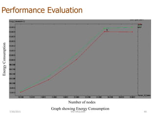
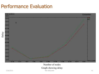
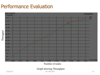
This document presents a delay constrained routing algorithm for wireless sensor networks with a mobile sink. It begins with an introduction to sensor nodes, wireless sensor networks, and the challenges of routing in WSNs. It then discusses prior work on stationary and mobile sink approaches. The proposed work formulates the problem and solves it using an optimal traveling salesman tour calculation and variable sojourn time computation. Simulation results show the proposed algorithm outperforms an existing MILP approach in terms of throughput, delay, energy consumption and network lifetime.