Download to read offline
![IJRET: International Journal of Research in Engineering and Technology eISSN: 2319-1163 | pISSN: 2321-7308
_______________________________________________________________________________________
Volume: 03 Issue: 07 | Jul-2014, Available @ http://www.ijret.org 335
APPROACHES TO THE NUMERICAL SOLVING OF FUZZY
DIFFERENTIAL EQUATIONS
D.T.Muhamediyeva1
1
Leading researcher of the Centre for development of software products and hardware-software complexes, Tashkent,
Uzbekistan
Abstract
One of the main problems of the theory of numerical methods is the search for cost-effective computational algorithms that
require minimal time machine to obtain an approximate solution with any given accuracy. In article considered fuzzy analog of
the alternating direction, combining the best qualities of explicit and implicit scheme is unconditionally stable (as implicit
scheme) and requiring for the transition from layer to layer a small number of actions (as explicit scheme).
Keywords: fuzzy set, quasi-differential equation, the scheme of variable directions, finite-difference methods.
--------------------------------------------------------------------***------------------------------------------------------------------
1. INTRODUCTION
The concept of fuzzy differential equations was introduced
by O.Kaleva in 1987. In [1] he proved the theorem of
existence and uniqueness of solutions of such equations.
Later in [2-6] were been obtained properties of fuzzy
differential equations and their solutions. To determine
fuzzy derivative O.Kaleva used M.L.Pur and D.A.Rulesku’s
approach [7] to the differentiability of fuzzy mappings,
which, in turn, is based on the M.Hukuhara’s idea [8] about
differentiability of multivalued mappings. In this regard, the
O.Kaleva’s approach adopted all the shortcomings typical
differential equations with the Hukuhara’s derivative.
In 1990 J.P.Aubin [9] and V.A.Baidosov [10,11] introduced
into consideration fuzzy differential inclusion. Their
approach to solving such equations is based on the latest
information for ordinary differential inclusions. In the
future, fuzzy inclusion were considered in works [12-15].
In [17], in the same way as was done in the theory of
differential equations with multivalued right-hand side [16],
introduced the concept of quasi-differential equation. This
allows on the one hand to avoid the difficulties that arise in
the solution of fuzzy differential equations and inclusions,
and with other - to get some of their properties by available
methods.
2. STATEMENT OF THE TASK
Let )( n
RConv - the space of nonempty convex compact
subsets
n
R with Hausdorf metric
gfgfGFh
FfGgGgFf
infsup,infsupmax),( ,
Where, under refers Euclidean norm in space
n
R .
Now we introduce the space
n
E of the mapping
]1,0[: n
R , which satisfying the following
conditions:
1. - semi-continuous from above, i.e. for any
n
Rx '
and for any 0 there is 0),'( x such that for all
'xx runs condition )'()( xx ;
2. - normally, i.e. there exists a vector
n
Rx 0 such
that 1)( 0 x ;
3. - fuzzy convex, i.e. for any
n
Rxx '',' and any
]1,0( true inequality
)}''(),'(min{)'')1('( xxxx ;
4. The closure of the set 0)( xRx n
is compact.
Zero in the space
n
E are elements
0,0
0,1
)( n
Rx
x
x
Definition 1 - cutting
][ of the mapping
n
E at
10 let's call a set )(xRx n
. Zero
cutting of the map
n
E let's call the closure of the set
0)( xRx n
.
Let’s define in space
n
E metric ),0[: nn
EED ,
fancy )][,]([sup),(
10
hD
.
Definition 2 Mapping
n
ETf ],0[: called weakly
continuous at the point ),0(0 Tt , if for any fixed](https://image.slidesharecdn.com/approachestothenumericalsolvingoffuzzy-140821043813-phpapp01/75/Approaches-to-the-numerical-solving-of-fuzzy-1-2048.jpg)
![IJRET: International Journal of Research in Engineering and Technology eISSN: 2319-1163 | pISSN: 2321-7308
_______________________________________________________________________________________
Volume: 03 Issue: 07 | Jul-2014, Available @ http://www.ijret.org 336
]1,0[ and arbitrary 0 there is 0),( such
that ))(),(( 0tftfh for all ],0[0 Tt such, that
),(0 tt .
Definition 3 Integral of the mapping
n
EIf : over the
interval I is the element
n
Eg such that
I
dttfg )(][
for all ]1,0( .
Definition 4 Mapping
n
EIf : called differentiable at
the point It 0 , if fr all ]1,0[ multivalued mapping
)(tf differentiable by Hukuhara [198] in the point 0t , its
derivative is equal to )( 0tfDH and the
]}1,0[:)({ 0 tfDH set family defines an element.
Definition 5 For
nn
EwEvu ,, called u and v , if
wvu , and it is written as vHuw .
Definition 6 Function
n
EbaF ],[: differentiable in
),(0 bat , if there is a
n
EtF )(' 0 such that there are
limits
h
tFHhtF
h
)()(
lim 00
0
and
h
htFHtF
h
)()(
lim 00
0
and they are equal to )(' 0tF .
If F differentiable in ),(0 bat , hen for all slices
)]([)( tFtF there is a Hukuhara differential in 0t and
)()]('[ 0 tDFtF
, where DF is called Hukuhara
differential F .
Definition 7 For function
n
Ebaf ],[: Seikkala
introduced the concept )(tSDf in a such way
10)],,(),,([)]([ '
2
'
1
tftftSDf .
For
)]([],,[ tSDfbat is fuzzy. If mapping
n
EIf : differentiable at the point It 0 , then
)(' 0tf call fuzzy derivative )(tf in the point 0t .
Mapping
n
EIf : called differentiable on I , if it is
differentiable at each point It .
Definition 8 Mapping
n
EIf : is called uniformly
continuous on
n
EG , if for each 0 there is
0)( such that for all Gyx , , satisfying the
inequality ),( yxD fair assessment
))(),(( yfxfD .
Definition 9 Fuzzy number u~ is called a fuzzy number of
RL type, if
( )
( ) 1 ,
( )
( )
( ) 1 ,
L
L
L
u
R
R
R
u u
u
u
u u
u
u
where u - clear value of the number u~ , i.e.
)1()1( RL uuu ; Lu and Ru respectively the left and
right stretching of fuzzy number u~ ; )(Lu and )(Ru -
respectively the left and right values of the fuzzy number u~
of definition .
From the definition it follows that if
)}(),(,{)(~ RL uuuu , then
LL uuu )1()( ; RR uuu )1()( .
Consider the algebraic action on fuzzy RL type:
Addition:
)})(1();)(1({~~
RRLL vuvuvuvuvu
.
Subtraction:
)})(1();)(1({~~
RRLL vuvuvuvuvu
.
Multiplication:
1) for 0;0 vu
})1())(1(;)1())(1(;{~~
LRRRLLLL vuvuuvvuvuuvvuvu ;
2) for 0;0 vu](https://image.slidesharecdn.com/approachestothenumericalsolvingoffuzzy-140821043813-phpapp01/75/Approaches-to-the-numerical-solving-of-fuzzy-2-2048.jpg)
![IJRET: International Journal of Research in Engineering and Technology eISSN: 2319-1163 | pISSN: 2321-7308
_______________________________________________________________________________________
Volume: 03 Issue: 07 | Jul-2014, Available @ http://www.ijret.org 337
})1())(1(;)1())(1(;{~~
LRRLLLLR vuvuuvvuvuuvvuvu ;
3) for 0;0 vu
})1())(1(;)1())(1(;{~~
LLLLRRLR vuvuuvvuvuuvvuvu .
Division:
v
u
v
u
~
1~
~
~
.
Definition 10 We say that the mapping
nn
EET ],0[],0[],0[: specifies the local
quasi movement, if satisfied following conditions:
1) initial conditions axiom yyt ),,0,0( ;
2) quasiprimitive axiom:
)(0)),,,(),,0,,(( 110 hythyhD NmmN
,
Where
m
s
s
N
n
n thh
01
;
3) axiom of continuity: mapping
)),(,,( txyh is - weakly continuously.
Approximation equation
),(0))),(,,,(),,(( htxyththxyD
,
Dxxuxy ,)()0,( 0 ,
],0[,),,(),( Ttxtxtxy
we will call fuzzy quasi-differential equation.
Definition 11 Continuous map
n
T EQy : , satisfying
the approximation equation will be called a solution of fuzzy
quasi-differential equation.
In this paper discusses some of the issues of building fuzzy
analogs of finite difference methods.
Let’s consider the initial-boundary task
TQtxtxfLu
t
u
),(),,( , (1)
,),()0,( 0 Dxxuxu (2)
],0[,),,(),( Ttxtxtxu , (3)
2
2
2
22
1
2
121 ,,
x
u
uL
x
u
uLuLuLuLu
,
2,1;0 lxD ,
),(],,0( 21 xxxTDQT .
Suppose that ),(),,(),(0 txftxxu - are fuzzy functions.
)]([)( 0
]1,0[
0 xUxu
,
,)],([),(
]1,0[
txtx
(4)
]1,0[,)],([),(
]1,0[
txFtxf (5)
We introduce two-dimensional spatial grid and temporary
one-dimensional grid:
)],([,;5,0
,2,1;0;),(
2
1
1
2
1
,
2121
s
n
s
s
s
nnhhhhh
txfyyttt
NnDxxwww
In this case, the construction of the discrete solution of the
task (1)-(5) is reduced to the definition in the grid of fuzzy
numbers
][ s
y , such, that for for exact solutions ),( txu
of the task (1)-( 3) with any initial condition
)]([)( 0
]1,0[
0 xUxu
and](https://image.slidesharecdn.com/approachestothenumericalsolvingoffuzzy-140821043813-phpapp01/75/Approaches-to-the-numerical-solving-of-fuzzy-3-2048.jpg)
![IJRET: International Journal of Research in Engineering and Technology eISSN: 2319-1163 | pISSN: 2321-7308
_______________________________________________________________________________________
Volume: 03 Issue: 07 | Jul-2014, Available @ http://www.ijret.org 338
,)],([),(
]1,0[
txtx
fair inclusions
][),(
]1,0[
s
s ytxu
.
Let the function ]1,0[,)],([),(
]1,0[
txFtxf
defined for points TQtx ),( and ),( txF satisfies the
following conditions:
1)
)],([ txF - defined and continuous for all TQtx ),( .
2)
)],([ txF - monotonously to inclusion of 0h , i.e. from
2121 , TTXX ensue
)],([)],([ 2211 TXFTXF .
3) There is a real constant 0l , such that when
TQtx ),( true inequality
))]([)]([())],(([
txltxF .
Describe the fuzzy variant of the finite-difference methods
for tasks (1)-(5).
3. FUZZY VARIANT OF THE FINITE-
DIFFERENCE METHODS.
Replace differential operators with finite-difference:
2,1,, ,21 xx
yyyyyLu .
One of the main problems of the theory of numerical
methods is the search for cost-effective computational
algorithms that require minimal time machine to obtain an
approximate solution with any given accuracy 0 .
As is known, the explicit scheme requires a lot of activity,
but its stability is at a sufficiently small time step, the
implicit scheme is unconditionally stable, but it requires a
large number of arithmetic operations.
We can build a system that combines the best of explicit and
implicit scheme is unconditionally stable (as implicit
scheme) and requiring for the transition from layer to layer a
small number of actions (as explicit scheme).
One of the first cost-effective schemes is the scheme of
variable directions, built in 1955 by Pismen and Recordon.
Pismen and Reckford scheme makes the transition from
layer S on a layer 1S in two steps, using intermediate
(fractional) layer.
][][][
5,0
][][
2
2
1
1
2
1
ss
s
s
s
yy
yy
,
(6)
][][][
5,0
][][
2
2
1
1
2
1
1
ss
s
s
s
yy
yy
,
(7)
hwxxUxy ,)]([)]0,([ 0
, (8)
Nnnys
22
1
,0,][][
, (9)
Nnny
s
21
2
1
,0,][][
. (10)
Equation (6) is implicit in the first direction and clear for the
second, and equation (7) is explicit in the first direction, and
implicit in the second.
From (6) and (7) we get
][][][
2
][;][][][
2
1 yyFFyy ,
][][][
2
][;][]ˆ[]ˆ[
2
12 yyFFyy ,
1,...,2,1,][][
1
][
11
2][
1
1112
1
2
1
12 1111
NnFy
h
y
h
y
h
nnnn
,
111 ,0;][][ 11
Nnny nn
.
1,...,2,1,][]ˆ[
1
]ˆ[
11
2]ˆ[
1
2212
2
2
2
12 2222
NnFy
h
y
h
y
h
nnnn
,
222 ,0;][][ 22
Nnny nn
,
][][),,( 212211 nnn FFhnhnx ,
][][ 21nnyy .
Thus, the construction of the discrete solution of problem
(1)-(5) is reduced to the definition in the grid of fuzzy
numbers
][ s
y , such that for exact solutions ),( txu of the
task (1)-(3) with any initial condition
)]([)( 0
]1,0[
0 xUxu
and
,)],([),(
]1,0[
txtx
fair inclusions
][),(
]1,0[
s
s ytxu
.](https://image.slidesharecdn.com/approachestothenumericalsolvingoffuzzy-140821043813-phpapp01/75/Approaches-to-the-numerical-solving-of-fuzzy-4-2048.jpg)
![IJRET: International Journal of Research in Engineering and Technology eISSN: 2319-1163 | pISSN: 2321-7308
_______________________________________________________________________________________
Volume: 03 Issue: 07 | Jul-2014, Available @ http://www.ijret.org 339
4. NUMERICAL EXPERIMENT
Let’s consider the idea of the alternating direction method of
class cheap schemes, applied to the solution of the first
initial-boundary value task for two-dimensional heat
equation.
[ ( )] ( ) [ ] ( ) [ ]z y
u u u u
q z k w k au
t z z z y y
,
),0(),(),0(),,( TMMLtyz ,
),(],0[),(,)],([)]0,,([ MMLyzyzyzu
- initial conditions,
Ttyztyztyzu 0,),(,)],,([)],,([
-
boundary conditions
где ),,(),0( MML is - domain border;
)],,([,)],([ tyzyz - - sections of the set of fuzzy
functions. TML ,, - given numbers.
Initial equation is approximated by the combination of two
difference schemes, each of which corresponds to only one
spatial direction. Each element of the sum approximated by
explicit and implicit structures.
To do this, along with a layer
n
tt , alculation of which is
carried out at this stage, the inclusion of an additional layer
2
1
n
tt . Then for the transition from layer
n
tt to the
layer
1
n
tt by using the layer 2
1
n
tt the original
differential equation is approximated by two differential
equations, one of which connects layers
n
tt and
2
1
n
tt , and the second layers 2
1
n
tt and
1
n
tt .
First phase. Transition to more smart
2
1
n - th layer with
step
2
. Time derivative is approximated by the formula
2
ˆˆ
),,(
2
1
n
ij
n
ijn
jit
uHu
tyzu
,
Derivative by z approximated on
2
1
n - th layer,
derivative by y on n - th layer.
Included in the right part of the initial equation fuzzy
function
)],,,([ qtyzf is replaced by its grid view.
Corresponding difference scheme has the form:
,11,11,ˆ
2
ˆˆ)(ˆ
2
ˆˆˆˆ)(ˆ
2
ˆˆ
2
1
2
1,1,
2
1
,1
2
1
,1
2
2
1
,1
2
1
2
1
,1
2
1
11
11
JjIiu
a
h
ukukkuk
h
uu
w
h
ukukkukuu
q
n
ij
y
n
jiy
n
ijyy
n
jiy
z
n
ji
n
ji
z
n
jiz
n
ijzz
n
jiz
n
ij
n
ij
i
jjjj
iiii
Where
)
2
1
,,(ˆˆ 2
1
n
ii
n
ij tyzuu or in traditional recording
,11,11,ˆ
42
ˆ
422
ˆ
42
2
1
,12
2
1
22
2
1
,12
1
1
JjIiFuw
h
k
h
u
a
qk
h
k
h
uw
h
k
h
n
ij
n
ji
z
z
z
n
ijiz
z
z
z
n
ji
z
z
z
i
iii
(11)](https://image.slidesharecdn.com/approachestothenumericalsolvingoffuzzy-140821043813-phpapp01/75/Approaches-to-the-numerical-solving-of-fuzzy-5-2048.jpg)
![IJRET: International Journal of Research in Engineering and Technology eISSN: 2319-1163 | pISSN: 2321-7308
_______________________________________________________________________________________
Volume: 03 Issue: 07 | Jul-2014, Available @ http://www.ijret.org 342
defined
iu
Then we have
ii uu ˆ
Where
,
2 2
jy
y
i k
h
a
,
422 122
a
qk
h
k
h
b iy
y
y
y
i jj
,
2 12
jy
y
i k
h
c
2
1
n
iji Qf в (2) и
,
42 2
w
h
k
h
a
z
z
z
i i
,
422 122
a
qk
h
k
h
b iz
z
z
z
i ii
,
42 12
w
k
k
h
c
z
z
z
i i
n
iji Ff .
5. CONCLUSIONS
Introduced analogues of numerical solutions of fuzzy
differential equations by the method of variable directions
generalize earlier reviewed fuzzy differential equations and
inclusions and provide an opportunity to examine their
properties.
REFERENCES
[1]. Kaleva, O. Fuzzy differential equations / O. Kaleva //
Fuzzy Sets and Systems. — 1987. — Vol. 24, № 3. — P.
301 — 317.
[2].Комлева, Т.А. Усреднение нечетких
дифференциальных уравнений / Т.А. Комлева, А.В.
Плотников, Л.И. Плотникова // Тр. Одес. политех. ун-та.
— Одесса, 2007. — Вып. 1(27). — С. 185 — 190.
[3]. Kaleva, O. The Peano theorem for fuzzy differential
equations revisited / O. Kaleva // Fuzzy Sets and Systems.
— 1998. — № 98. — P. 147 — 148.
[4]. Kaleva, O. O notes on fuzzy differential equations / O.
Kaleva // Nonlinear Analysis. — 2006. — № 64. — P. 895
— 900.
[5]. Park, J.Y. Existence and uniqueness theorem for a
solution of fuzzy differential equations / J.Y. Park, H.K. Han
// Internat. J. Math. and Math. Sci. — 1999. — Vol. 22, №
2. — P. 271 — 279.
[6]. Park, J.Y. Fuzzy differential equations / J.Y. Park, H.K.
Han // Fuzzy Sets and Systems. — 2000. — № 110. — P. 69
— 77.
[7]. Puri, M.L. Differential of fuzzy functions / M.L. Puri,
D.A. Ralescu // J. Math. Anal. Appl. — 1983. — № 91. —
P. 552 — 558.
[8]. Hukuhara, M. Integration des applications mesurables
dont la valeur est un compact convexe / M. Hukuhara //
Func. Ekvacioj. — 1967. — № 10. — P. 205 — 223.
[9]. Aubin, J.P. Fuzzy differential inclusions / J.P. Aubin //
Problems of Control and Information Theory. — 1990. —
Vol.19, № 1. — P. 55 — 67.
[10]. Baidosov, V.A. Differential inclusions with fuzzy
right-hand side / V.A. Baidosov // Soviet Mathematics. —
1990. — Vol. 40, № 3. — P. 567 — 569.
[11]. Baidosov, V.A. Fuzzy differential inclusions / V.A.
Baidosov // J. of Appl. Math. and Mech. — 1990. — Vol.
54, № 1. — P. 8 — 13.
[12]. Hullermeir, E. An approach to modeling and
simulation of uncertain dynamical systems / E. Hullermeir //
Int. J. Uncertainty Fuzziness Knowledge Based Systems. —
1997. — № 5. — P. 117 — 137.
[13]. Lakshmikantham, V. Interconnection between set and
fuzzy differential equations / V. Lakshmikantham, S. Leela,
A.S. Vatsala // Nonlinear Analysis. — 2003. — № 54. — P.
351 — 360.
[14]. Lakshmikantham, V. Theory of set differential
equations in metric spaces / V. Lakshmikantham, T. Granna
Bhaskar, J. Vasundhara Devi — Cambridge Scientific
Publishers, 2006. — 204 p.
[15]. Lakshmikantham, V. Existence and interrelation
between set and fuzzy differential equations / V.
Lakshmikantham, A.A. Tolstonogov // Nonlinear Analysis.
— 2003. — № 55. — P. 255 — 268.
[16]. Панасюк, А.И. Квазидифференциальные уравнения
в метрическом пространстве / А.И. Панасюк //
Дифференциальные уравнения. — 1985. — Т. 21, № 8.
— pp. 1344 — 1353.
[17]. Комлева Т.А., Плотников А.В., Плотникова Л.И.
Нечеткие квазидифференциальные уравнения. // Тр.
Одес. политех. ун-та. — Одесса, 2008. — Вып. 2(30). —
p. 207 — 211.](https://image.slidesharecdn.com/approachestothenumericalsolvingoffuzzy-140821043813-phpapp01/75/Approaches-to-the-numerical-solving-of-fuzzy-8-2048.jpg)

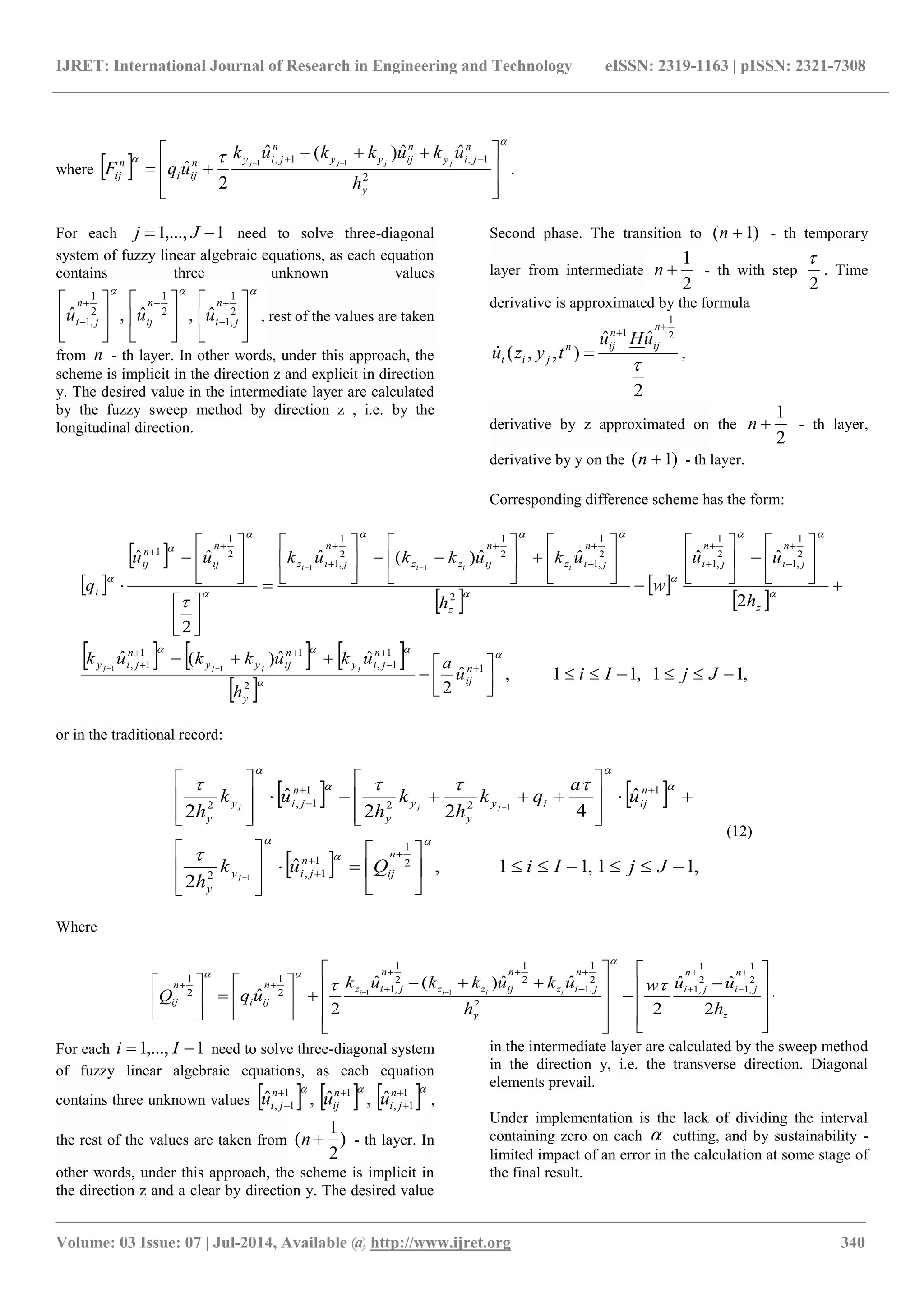
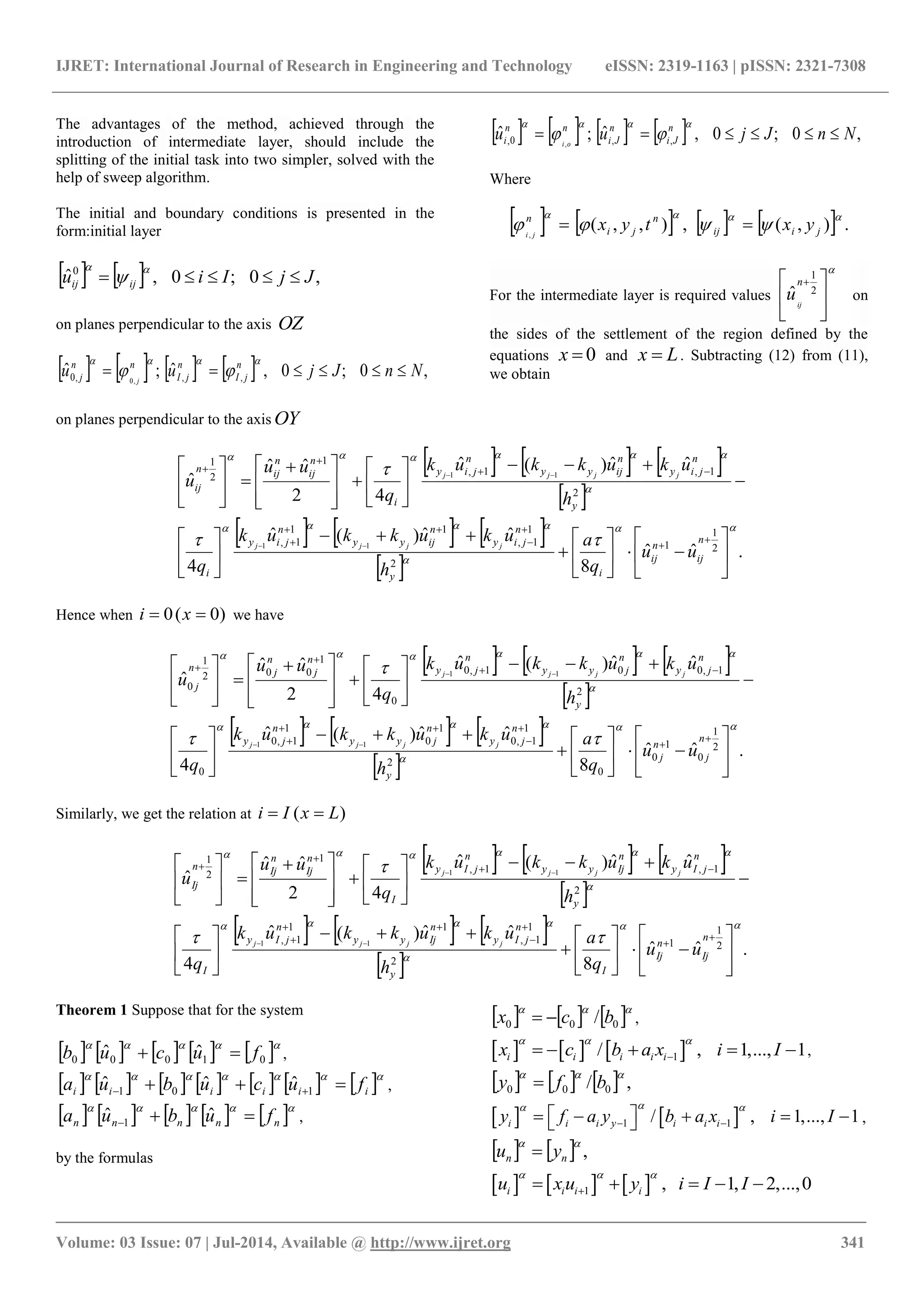
This document summarizes approaches to numerically solving fuzzy differential equations. It begins by introducing fuzzy differential equations and discussing previous work in the area. It then defines key concepts related to fuzzy sets, fuzzy derivatives, and quasi-differential equations. The document proposes using finite difference methods to build fuzzy analogs for solving initial-boundary value problems involving fuzzy differential equations. It describes setting up spatial and temporal grids and defining discrete fuzzy number solutions that approximate the exact solutions to the fuzzy differential equations.


![11.[8 17]numerical solution of fuzzy hybrid differential equation by third or...](https://cdn.slidesharecdn.com/ss_thumbnails/11-8-17numericalsolutionoffuzzyhybriddifferentialequationbythirdorderrungekuttanystrommethod-120512235447-phpapp02-thumbnail.jpg?width=640&height=640&fit=bounds)


![ANPARA THERMAL POWER STATION[1] sangam.pdf](https://cdn.slidesharecdn.com/ss_thumbnails/anparathermalpowerstation1sangam-251121115219-9261cde4-thumbnail.jpg?width=640&height=640&fit=bounds)


