Estudo Doppler

1. Application of a Side-Looking (SL) Doppler Flow Meter for
Measuring Discharge on the Southern Leg of the Parana’ River at
the Entrance to the Itaipu Binacional Reservoir, Parana’, Brasil
BY
Paulo E. Gamaro, Hydrologist, Itaipu Binacional,.
Introduction
Variable backwater effects are common in low-gradient rivers, large and small rivers
in proximity of the entrance to reservoirs (Parana’ River entrance to Itaipu Reservoir),
and the confluence of large and small rivers (the Igauçu Rivers confluence with the
Parana’ River below Itaipu Binacional Hydroelectric Dam). The continuous
measurement of discharge using a traditional relation of water level (stage) to
discharge is complicated by the unsteady variable backwater effect.
A traditional method of continuous discharge measurements in upland type rivers is
the development of a relation of stage to discharge. This method is based on the
following assumptions: (1) a reasonably stable channel or control section, (2) little or
no variable backwater effect, (3) consistent energy gradient (no flow reversals), (4)
gravity is the principle driving force (rate of change of momentum is not great; Sloat
and Gain, 1995). These assumptions are not all met on the Parana’ River near the
entrance to the Itaipu Binacional Reservoir because of the backwater conditions
caused by the Itaipu Reservoir.
A second method to continuously measure discharge is to measure a stable section of
velocity in the river (index velocity), relate the index velocity to the mean river
velocity, and multiply the cross-sectional area by the computed mean velocity. An
index velocity can be measured at either a point or along in a horizontal and/or
vertical section in the river.
In an effort to improve the accuracy of the discharge records on the Parana’ River
near its entrance to the Itaipu reservoir, Itaipu Binacional in cooperation with SonTek,
Inc. instrumented the site with a Argonaut Side-Looking (SL) Doppler Flow meter
between April 4th
and May 18th
, 2001. Evaluation of existing discharge records
indicated that simple stage-only relations of discharge (described in Rantz, and others,
1982) were not appropriate because of the variable backwater effect. The decision by
Itaipu Binacional to instrument this site was based on previous examination of
complex discharge measurement sites in the USA operated by the U.S. Geological
Survey (USGS) Water Resources Division, tow-tank tests of the Argonaut SL in both
the Navy tow basin in Escondido, CA (SonTek, 1997) and at the U.S. Geological
Survey Hydrologic Instrumentation Facility (HIF; SonTek, 2001) which proved that
the Argonaut SL could be used to develop accurate and reliable discharge records.
Presently, there are over 250 ADVMs used in North America to measure discharge
using the index-velocity method.
This is the first one in Brazil.

2. Purpose and Scope
This report describes the installation of the Argonaut SL and computation methods
applied to report continuous records of discharge on the Southern Leg of the Parana’
River near its entrance to the Itaipu Reservoir. The installation and programming of
the Argonaut SL are discussed. The development of ratings to compute discharge are
described including bathymetric surveys for channel area, continuous measurement of
an index velocity using a Argonaut SL, discrete discharge measurements used for
rating development, development of stage-area curves, statistical estimation of the
relation of mean velocity and Argonaut SL-measured index velocity, and computation
of instantaneous discharge.
Application of a Side-Looking (SL) Doppler Flow Meter
for Measuring Discharge at the Confluence of the
Parana’ River and the Itaipu Binacional Reservoir
The application of Argonaut SLs for computing records of discharge in variable
backwater rivers includes several topics directly related to the use of the Argonaut SL.
These are: (1) Principles of Acoustic Doppler Flow Meters, (2) Installation of the
Argonaut SL, and, (3) computation of discharge. Each topic is discussed in the
following sections.
Principles of Acoustic Doppler Velocity Measurement using
the Argonaut Side-Looking Flow Meter
The Argonaut SL flow meter measures the velocity of water using a physical principle
called the Doppler shift. This states that if a source of sound is moving relative to the
receiver, the frequency of the sound at the receiver is shifted from the transmit
frequency.
C
V
FF sd 2−=
Where:
Fd = change in received frequency (Doppler shift), in units of Hz;
Fs = frequency of transmitted sound, in units of Hz;
V = velocity of source relative to receiver, (i.e. motion that changes the
distance between the two). Positive V corresponds to the increasing
distance; and,
C = speed of sound.
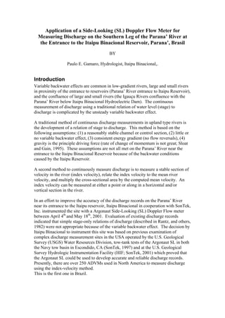
Figure 1 illustrates the operation of a monostatic Doppler current meter, such as the
Argonaut SL. The term monostatic refers to the fact that the same transducer is used

3. as transmitter and receiver. The transducer generates a short pulse of sound at a
known frequency, which propagates through the water. The transducer is constructed
to generate a narrow beam of sound where the majority of energy is concentrated in a
cone a few degrees wide. As the sound travels through the water, it is reflected in all
directions by particulate matter (sediment, biological matter, bubbles, etc.). Some
portion of the reflected energy travels back along the transducer axis, where the
transducer receives it and the Argonaut SL measures the change in frequency of the
received signal. The Doppler shift measured by a single transducer reflects the
velocity of the water along the axis of the acoustic beam of that transducer. If the
distance between the transducer and the target is decreasing, frequency increases; if
the distance is increasing, frequency decreases (Figure 1). Motion perpendicular to the
line connecting source and receiver has no effect on the frequency of received sound.
The location of measurements made by a monostatic Doppler current meter is a
function of the time at which the return signal is sampled. The time since the pulse
was transmitted determines how far the pulse has propagated, and thus specifies the
location of the particles that are the source of the reflected signal. By measuring the
return signal at different times following the transmit pulse, the Argonaut SL
measures the water velocity at different distances from the transducer.
Figure 1. – The operation of the Argonaut SL monostatic Doppler current
meter.
The Argonaut SL is designed for horizontal side-looking operation from underwater
structures, but can also be used for vertical up or down-looking installations in narrow
channels. The measurement volume is a V-shaped wedge in the plane defined by the
two acoustic beams. The sides of the V are sloped 25° off the horizontal axis of the
instrument. The width of the V is equal to 0.93 times the range from the transducer
head (at 20 m the width is 19.3 m). The limits of the measurement volume (range) are
determined by user selected parameters. This range is defined by two parameters:
“Cell Begin” and “Cell End”. Both are given in distance from the transducers along
the axis of the instrument; the minimum difference between the two is 0.5 meters, the
maximum distance between the two is 21.5 meters. The Argonaut SL can be
programmed to collect data in a “profiling-mode” with up to five individual
measurements of water-velocity (show in figure 2) at equal widths away from the

4. transducers face, or in a “single volume-mode” outputting a single velocity
measurement averaged over the entire sample volume. Figure 2 show a plan and
cross-sectional view of a typical Argonaut SL installation. The diagram shows the
beam orientation, the location of the horizontal and vertical transducers for water
velocity and water level measurement, respectively, and a generalized water velocity
sample volume measured by the Argonaut SL.
Vx
5Vx
4Vx
3Vx
2Vx
1
1.5-MHz Argonaut SL
Cross-section (side) view
Water Velocity Measurement
Volume
Water-surface
(level)
Acoustic Water level Measurement
Acousti
c
Beam 2
Acoustic
Beam 1
X-
axis
Vertical Acoustic Beam
Plan
View
Y-
axis
1.5 Mhz Argonaut SL
Flow
Directio
n
Figure 2. Plan- and Cross-sectional view of Argonaut SL transducer orientations and
water level and velocity measurement sample volumes.
Description of the Argonaut SL Discharge
Measurement Site
Preliminary reviews were done by hydrologists at Itaipu Binacional to determine the
best location for the Argonaut SL installation. Taken into consideration were:
logistics and access to the site, construction and installation of the mount, safety, and
instrument clearance.
The Argonaut SL was installed near the right bank (when facing downstream) in the
southern section of the Parana’ River about 5-Km upstream of the entrance into the
Itaipu Binacional reservoir. The flow in the Parana’ River in this section experiences
variable back water conditions caused by the large reservoir immediately

5. downstream. The width of the Parana’ River at this location is approximately 890
meters in width and has an average depth of 6-meters.
Equipment and Installation Description
The installation and setup was very simple and required only a few mounting parts to
be complete. The Argonaut SL used in this evaluation measures water-velocity, water
level, temperature, and battery voltage and records data to an internal 2-Mb data
recorder (80,000 lines of data). The Argonaut SL was powered using an external 12-
volt battery connected to a small 10-watt solar panel and regulator. A 10-meter
waterproof cable connects the instrument to power supply and communications from
shore. Figure 3. shows the storage shelter used to protect the battery from vandalism
and the weather. Figure 4a and b. shows a picture of the Argonaut SL being installed
on the Parana’ River by hydrologic technicians from Itaipu Binacional. The entire
installation including performing instrument diagnostics and measurement
programming required less than one hour to complete.
Figure 3. Argonaut SL battery shelter (Parana’ River)
Figure 4a. – Argonaut SL installation
(Parana’ River)
. Figure 4b. Argonaut SL attached to mounting bracket.

6. The Argonaut SL was installed using a prefabricated mount (as shown in figure 4.). A 10-
meter power/communications cable attached to the Argonaut SL runs up to the storage shelter
where the battery is located (cable lengths can be up to 100-meters using a standard SonTek
cable). The primary requirement for the pre-fabricated mount was that it is very sturdy and
will not move during the deployment. The mount was also designed such that the instrument
can easily be removed.
The Argonaut SL was aligned in the river such that the downstream flow was parallel to the
face of the instrument. It was installed 0.75 meters below the water-surface (as show in figure
4b) to prevent acoustic reflections from the water-surface.
The Argonaut SL was sampled at 10-minute intervals. Once activated, the Argonaut SL
measured velocity and water level at 1-Hz (once sample per second) during a 2-minute
period. The velocity sample volume for velocity ranged from 0.5 meters to 20.0 meters away
from the face of the transducer. All data including water velocity, water level, standard
deviations, signal strength, temperature, and voltage are recorded with each sample to the
internal 2-Mb data recorder.
Discharge Measurements for Calibration
Discharge was measured at the site to determine mean velocity using an Acoustic Doppler
Profiler (ADP). The ADP was mounted from a small boat and transected across the river
section in about 5 – 7 minutes. The ADP was used to measure discharge because of the
limitations of the more common mechanical current meters that take more than 3 – 4 hours to
complete a single measurement (Rantz and others, 1982, v. 1, p.86). Because of the rapidly
changing flow caused by the variable backwater condition at the measurement site
measurements of mean velocity had to be made as quickly as possible.
A minimum of four discharge measurements was performed during each calibration and then
averaged. During each discharge measurement, the Argonaut SL measured water level and
index-velocity for 2-minutes at 10-minute intervals.
Three sets of discharge measurements were made during this study. Following table provides
a summary of the discharge results:
Date Discharge (m3
/s) Number of
measurements
Standard deviation
(m3
/s)
April 5, 2001 2,372 4 9
April 18, 2001 2,268 4 22
May 5, 2001 2,070 6 26
Development of Discharge Rating Curve
Discharge of a river is computed as the product of the mean velocity and cross-sectional area:
MAVQ =

7. where Q is discharge, in cubic meters per second,
A is cross-sectional area, in square meters,
VM is mean velocity, in meters per second.
Considering complex flow conditions that exist when variable backwater is present, it is
necessary to develop a relation for area and velocity. These relations are developed using
measurable variables such as water level and velocity (Sloat and Gain, 1995). Cross-sectional
area can be expressed as a function of water level. Mean velocity can be expressed as a
function of specific stream variables including: water level, index velocity, and rate of change
of water level and water velocity (Sloat and Gain, 1995).
Least-Squares multiple-linear regression is a good tool to use for the development of the area
and mean velocity relation. In addition, residuals (unexplained error) from the regression
equations can be used to determine if a significant relation exists between the mean velocity
(response variable) and index velocity (independent variable) and if the response variable is
adequately estimated. Draper and Smith (1982) describe this regression method and residual
analysis.
Water-Level/Cross-sectional Area Relation
Itiapu Binacional had previously developed a water level relation at the study site. The cross-
sectional area was computed as a function of water level using a bathymetric survey of the
channel (measured using a fathometer) at various water levels. Cross-sectional are was
computed for values of water level ranging between the minimum and maximum water levels
expected at the site. A table defining the relation was then developed. The following graph
shows the water-level/cross-sectional area relation for the study site.
Parana' River (southern leg)
0.00
1000.00
2000.00
3000.00
4000.00
5000.00
6000.00
7000.00
0.00 1.00 2.00 3.00 4.00 5.00
Water level, in meters
Cross-sectionalArea,in
squaremeters
Table 1. – Relation between water level and cross-sectional area for Argonaut SL discharge
study site.
Mean-Velocity Rating using the Index-Velocity Method
A regression equation was developed relating mean velocity computed from discharge
measurements to corresponding Argonaut SL index velocity measurements. For a permanent
station, data should be collected during periods of seasonal high and low flow (Rantz and
others, 1982). The regression analysis required several assumptions about errors calculated

8. from the regression (as documented in Sloat and Gain, 1995): errors must be independent
over time (not serially correlated), normally distributed, and of equal variance over the range
of values. It should be noted that the mean velocity and index-velocity data used in the
regression analysis was limited due to the short duration of the evaluation. Actual estimates of
error would require several more data points collected throughout the year.
The regression equation was initially developed using mathematical combinations of stage
and Argonaut SL index-velocity. The results indicate that Argonaut SL index velocity was
the only significant linear predictor of mean velocity. The general form of the regression
equation for the study site is:
bVaV IM +∗=
where VM is mean velocity in meters per second,
VI is index velocity measured from the Argonaut SL, in meters
per second, and,
a and b are constants.
The relation between mean velocity and Argonaut SL measured index-velocity is shown in
figure 5. Mean velocity was computed by dividing measured discharges by cross-sectional
area from the water level-area rating for the average stage during the discharge measurement.
Although the data is very limited, it does indicate that the measured mean velocity can be
expressed as a simple linear function of Argonaut SL index-velocity. With additional
measurements descriptive statistics including the standard error of estimate for the regression
and a residual analysis can be used for analysis to better determine the significance of the
relation between mean velocity and index velocity and to ensure that the mean velocity is
adequately estimated. Sloat and Gain, 1995, describe this analysis method and approach in
more detail.
Figure 6. – Relation of mean-velocity in the Parana’ River (southern leg) to Argonaut SL-
measured index velocity for Parana’ River discharge measurement study site.
Parana' River (southern leg)
0.3
0.4
0.5
0.6
0.7
0.1 0.2 0.3 0.4
Argonaut SL Index-velocity, in meters per second
Meanvelocity,inmeterspersecond
Y
Predicted Y

9. Results of Discharge Computations Using Data Collected by
the Argonaut SL
Discharge was computed as the product of the cross-sectional area (computed from the water
level-cross-sectional area relation) and mean-velocity (computed from the mean velocity-
Argonaut SL measured Index velocity relation). Figure 7. shows a time-series plot discharge,
water-level, temperature, and velocity collected by the Argonaut SL at the study site.
The data indicate that although the water level and discharge respond in a relatively similar
pattern, values of discharge fluctuate rapidly on a very short time-scale relative to values of
water level. Values of index-velocity (used in the discharge computation) plotted on the
lower graph further support this trend. They can be seen fluctuating (pulsing) on average
about +/- 0.05 m/s between successive measurements. Some of this variation can be
attributed to the accuracy of the velocity measurement. The standard deviation of velocity
relation was 0.02 m/s (keeping in mind that this using a very limited data set), thus,
approximately 0.03 m/s could be attributed to the pulsing of flow as it enters the reservoir.
Again, as a very general estimate, considering an average cross-sectional area of about 4,250
cubic meters, this relates to an average fluctuation in flow of approximately 127 cubic meters
per second between successive 10-minute samples. The circles located in the upper plot
identify the most significant effects of the variable backwater flow condition at the site. They
show that for a given water level it is possible to have multiple values of discharge. This is a
primary example of errors that can be introduced by using a relation of water level to
discharge in a river that has variable backwater flow conditions. It also indicates that using
the “index-velocity” method (as described by Sloat and Gain, 1995 and Rantz and others,
1982 will accurately predict discharge without and errors (bias) caused by the variable
backwater flow condition.
Figure 7. – Time-series plot of discharge, water level, velocity, and temperature data collected
by the Argonaut SL on the Parana’ River (southern leg).

10. Summary
Index-velocity and water level data collected with a Side-Looking (SL) Doppler Flow Meter
and channel cross-sectional area data were used to compute discharge (using the index-
velocity method as described by Sloat and Gain, 1995) on the southern leg of the Parana’
Rivers entrance to the Itaipu Binacional Reservoir in Guaira, Parana’ State, Brasil. Discharge
was computed as the product of the channel area and mean velocity (computed from the index
velocity measured in the river by the Argonaut SL flowmeter).
Discharge measurements were made using an Acoustic Doppler Profiler (ADP) to compute
mean-velocity in the southern leg of the Parana’ River to the index velocity measured by the
Argonaut SL. Least-squares linear regression was used to develop a simple linear regression
between mean velocity and index velocity. Index velocity was the only significant linear
predictor of mean velocity for the flow measurement site on the Parana’ River.
Continuous discharge was computed by multiplying results of relations developed for cross-
sectional area and mean velocity. Principle sources of error in the estimate of discharge are
identified as: (1) Limited calibration measurements due to the short length of the study, (2)
instrument error associated with the measurement of water level and index-velocity by the
Argonaut SL, (3) errors in the representation of water level and index velocity due to the
natural variability of the stream in space and time, (4) errors in the cross-sectional area and
mean velocity ratings based on water level and index velocity. Mean daily discharge at the
measurement site ranged from 2,240 to 2,643 m3
/s during the 1 ½ month study period.
The results of discharge, water level, and index-velocity data measured by the Argonaut SL
during the study show that discharge fluctuates (pulses) on average about 127 cubic meters
per second between successive 10-minute measurements. In addition, the data clearly
indicate the presence variable backwater flow conditions at the study site. The data collected
by the Argonaut SL clearly indicate that using water level to predict values of discharge at
this site would produce variable errors. Further, the data collected by the Argonaut SL show
that the effects of the variable backwater flow condition are accounted for by using the
velocity index-method as described by Sloat and Gain, 1995 and Rantz and others, 1982.
Selected References
Chow, V.T., 1959, Open channel hydraulics: New York, McGraw-Hill, p. 523-535.
Draper, N.R., and Smith, Harry, 1982, Applied regression analysis: New York, John Wiley&
Sons, p. 141-210.
Rantz,S.E. and others, 1982, Measurement and computation of streamflow: v.1: Measurement
of stage and discharge, p. 174-175, and Computation of discharge: U.S. Geological Survey
Water-Supply Paper 2175, 631 p.
Sloat, J.V., Gain, W.S., 1995, Application of acoustic velocity meters for gauging discharge
of three low-velocity tidal streams in the St. Johns River Basin, Northeast Florida: U. S.
Geological Survey Water-Resources Investigation Report 95-4230, 26 p.
SonTek, Inc., 1999, Argonaut Side-Looking Doppler velocity meter principles of operation.