ANOVA Interpretation Set 1 Study this scenario and ANOVA.docx

ANOVA Interpretation Set 1
Study this scenario and ANOVA table, then answer the
questions in the assignment instructions.
A researcher wants to compare the efficacy of three different
techniques for memorizing
information. They are repetition, imagery, and mnemonics. The
researcher randomly assigns
participants to one of the techniques. Each group is instructed
in their assigned memory
technique and given a document to memorize within a set time
period. Later, a test about the
document is given to all participants. The scores are collected
and analyzed using a one-way
ANOVA. Here is the ANOVA table with the results:
Source SS df MS F p
Between 114.3111 2 57.1556 19.74 <.0001
Within 121.6 42 2.8952
Total 235.9111 44

9/10/2019 Print
https://content.ashford.edu/print/AUPSY325.16.1?sections=ch6,
ch6sec1,ch6sec2,ch6sec3,ch6sec4,ch6sec5,ch6sec6,ch6sec7,ch6
sec8,ch6summary,ch7,ch7sec1,ch7s… 1/76
Chapter Learning Objectives
After reading this chapter, you should be able to do the
following:
1. Explain why it is a mistake to analyze the differences
between more than two groups with
multiple t tests.
2. Relate sum of squares to other measures of data variability.
3. Compare and contrast t test with analysis of variance
(ANOVA).
4. Demonstrate how to determine significant differences among
groups in an ANOVA with more
than two groups.
5. Explain the use of eta squared in ANOVA.
6Analysis of Variance
Peter Ginter/Science Faction/Corbis

9/10/2019 Print
Introduction
From one point of view at least, R. A. Fisher was present at the
creation of modern statistical analysis. During
the early part of the 20th century, Fisher worked at an
agricultural research station in rural southern England.
Analyzing the effect of pesticides and fertilizers on crop yields,
he was stymied by independent t tests that
allowed him to compare only two samples at a time. In the
effort to accommodate more comparisons, Fisher
created analysis of variance (ANOVA).
Like William Gosset, Fisher felt that his work was important
enough to publish, and like Gosset, he met
opposition. Fisher’s came in the form of a fellow statistician,
Karl Pearson. Pearson founded the first department
of statistical analysis in the world at University College,
London. He also began publication of what is—for
statisticians at least—perhaps the most influential journal in the
field, Biometrika. The crux of the initial conflict
between Fisher and Pearson was the latter’s commitment to
making one comparison at a time, with the largest
groups possible.
When Fisher submitted his work to Pearson’s journal,
suggesting that samples can be small and many
comparisons can be made in the same analysis, Pearson rejected
the manuscript. So began a long and

increasingly acrimonious relationship between two men who
became giants in the field of statistical analysis and
who nonetheless ended up in the same department at University
College. Gosset also gravitated to the
department but managed to get along with both of them. Joined
a little later by Charles Spearman, collectively
these men made enormous contributions to quantitative research
and laid the foundation for modern statistical
analysis.
9/10/2019 Print
Try It!: #1
To what does the one in one-way ANOVA refer?
Joanna Zielska/Hemera/Thinkstock
If a researcher is analyzing how children’s
behavior changes as a result of watching a
video, the independent variable (IV) is
whether the children have viewed the video.
A change in behavior is the dependent
variable (DV), but any behavior changes
other than those stemming from the IV
reflect the presence of error variance.
6.1 One-Way Analysis of Variance
In an experiment, measurements can vary for a variety of

reasons. A study to determine whether children will
emulate the adult behavior observed in a video recording
attributes the differences between those exposed to the
recording and those not exposed to viewing the recording. The
independent variable (IV) is whether the children
have seen the video. Although changes in behavior (the DV)
show the IV’s effect, they can also reflect a variety
of other factors. Perhaps differences in age among the children
prompt behavioral differences, or maybe variety
in their background experiences prompt them to interpret what
they see differently. Changes in the subjects’
behavior not stemming from the IV constitute what is called
error variance.
When researchers work with human subjects, some level of
error variance is inescapable. Even under tightly
controlled conditions where all members of a sample receive
exactly the same treatment, the subjects are
unlikely to respond identically because subjects are complex
enough that factors besides the IV are involved.
Fisher’s approach was to measure all the variability in a
problem and then analyze it, thus the name analysis of
variance.
Any number of IVs can be included in an ANOVA.
Initially, we are interested in the simplest form of the
test, one-way ANOVA. The “one” in one-way
ANOVA refers to the number of independent
variables, and in that regard, one-way ANOVA is
similar to the independent t test. Both employ just one
IV. The difference is that in the independent t test the
IV has just two groups, or levels, and ANOVA can
accommodate any number of groups more than one.
ANOVA Advantage

The ANOVA and the t test both answer the same question: Are
there significant differences between groups? When one
sample is compared to a population (in the study of whether
social science students study significantly different numbers of
hours than do all university students), we used the one-sample
t test. When two groups are involved (in the study of whether
problem-solving measures differ for married people than for
divorced people), we used the independent t test. If the study
involves more than two groups (for example, whether working
rural, semirural, suburban, and urban adults completed
significantly different numbers of years of post-secondary
education), why not just conduct multiple t tests?
Suppose someone develops a group-therapy program for
people with anger management problems. The research
question is Are there significant differences in the behavior of
clients who spend (a) 8, (b) 16, and (c) 24 hours in therapy
over a period of weeks? In theory, we could answer the
question by performing three t tests as follows:
1. Compare the 8-hour group to the 16-hour group.
9/10/2019 Print
The Problem of Multiple Comparisons
The three tests enumerated above represent all possible

comparisons, but this approach presents two problems.
First, all possible comparisons are a good deal more manageable
with three groups than, say, five groups. With
five groups (labeled a through e) the number of comparisons
needed to cover all possible comparisons increases
to 10, as Figure 6.1 shows. As the number of comparisons to
make increases, the number of tests required
quickly becomes unwieldy.
Figure 6.1 Comparisons needed for five groups
Comparing Group A to Group B is comparison 1. Comparing
Group D to Group E would be the
tenth comparison necessary to make all possible comparisons.
The second problem with using t tests to make all possible
comparisons is more subtle. Recall that the potential
for type I error (α) is determined by the level at which the test
is conducted. At p = 0.05, any significant finding
will result in a type I error an average of 5% of the time.
However, the error probability is based on the
assumption that each test is entirely independent, which means
that each analysis is based on data collected from
new subjects in a separate analysis. If statistical testing is
performed repeatedly with the same data, the potential
for type I error does not remain fixed at 0.05 (or whatever level
was selected), but grows. In fact, if 10 tests are
conducted in succession with the same data as with groups
labeled a, b, c, d, and e above, and each finding is
significant, by the time the 10th test is completed, the potential
for alpha error grows to 0.40 (see Sprinthall,
2011, for how to perform the calculation). Using multiple t tests
is therefore not a good option.
Variance in Analysis of Variance

When scores in a study vary, there are two potential
explanations: the effect of the independent variable (the
“treatment”) and the influence of factors not controlled by the
researcher. This latter source of variability is the
error variance mentioned earlier.
The test statistic in ANOVA is called the F ratio (named for
Fisher). The F ratio is treatment variance divided by
error variance. As was the case with the t ratio, a large F ratio
indicates that the difference among groups in the
analysis is not random. When the F ratio is small and not
significant, it means the IV has not had enough impact
to overcome error variability.
Variance Among and Within Groups
9/10/2019 Print
If three groups of the same size are all selected from one
population, they could be represented by the three
distributions in Figure 6.2. They do not have exactly the same
mean, but that is because even when they are
selected from the same population, samples are rarely identical.
Those initial differences among sample means
indicate some degree of sampling error.
The reason that each of the three distributions has width is that
differences exist within each of the groups. Even
if the sample means were the same, individuals selected for the
same sample will rarely manifest precisely the

same level of whatever is measured. If a population is
identified—for example, a population of the academically
gifted—and a sample is drawn from that population, the
individuals in the sample will not all have the same
level of ability despite the fact that all are gifted students. The
subjects’ academic ability within the sample will
still likely have differences. These differences within are the
evidence of error variance.
The treatment effect is represented in how the IV affects what is
measured, the DV. For example, three groups of
subjects are administered different levels of a mild stimulant
(the IV) to see the effect on level of attentiveness.
The subsequent analysis will indicate whether the samples still
represent populations with the same mean, or
whether, as is suggested by the distributions in Figure 6.3, they
represent unique populations.
The within-groups’ variability in these three distributions is the
same as it was in the distributions in Figure 6.2.
It is the among-groups’ variability that makes Figure 6.3
different. More specifically, the difference between the
group means is what has changed. Although some of the
difference remains from the initial sampling variability,
differences between the sample means after the treatment are
much greater. F allows us to determine whether
those differences are statistically significant.
Figure 6.2: Three groups drawn from the same population
A sample of three groups from the same population will have
similar—but not identical—
distributions, where differences among sample means are a
result of sampling error.
Figure 6.3: Three groups after the treatment

Once a treatment has been applied to sample groups from the
same population, differences
between sample means greatly increase.
9/10/2019 Print
Try It!: #2
How many t tests would it take to make all
possible pairs of comparisons in a procedure
with six groups?
The Statistical Hypotheses in One-Way ANOVA
The statistical hypotheses are very much like they were for the
independent t test, except that they accommodate
more groups. For the t test, the null hypothesis is written
H0: µ1 = µ2
It indicates that the two samples involved were drawn from
populations with the same mean. For a one-way
ANOVA with three groups, the null hypothesis has this form:
H0: µ1 = µ2 = µ3
It indicates that the three samples were drawn from populations
with the same mean.

Things have to change for the alternate hypothesis, however,
because three groups do not have just one possible
alternative. Note that each of the following is possible:
a. HA: µ1 ≠ µ2 = µ3 Sample 1 represents a population with a
mean value different from the mean of the
population represented by Samples 2 and 3.
b. HA: µ1 = µ2 ≠ µ3 Samples 1 and 2 represent a population
with a mean value different from the mean of
the population represented by Sample 3.
c. HA: µ1 = µ3 ≠ µ2 Samples 1 and 3 represent a population
with a mean value different from the
population represented by Sample 2.
d. HA: µ1 ≠ µ2 ≠ µ3
All three samples represent populations with different means.
Because the several possible alternative outcomes
multiply rapidly when the number of groups
increases, a more general alternate hypothesis is
given. Either all the groups involved come from
populations with the same means, or at least one of
them does not. So the form of the alternate hypothesis
for an ANOVA with any number of groups is simply
HA: not so.
Measuring Data Variability in the One-Way ANOVA
We have discussed several different measures of data variability
to this point, including the standard deviation
(s), the variance (s2), the standard error of the mean (SEM), the
standard error of the difference (SEd), and the
range (R). Analysis of variance presents a new measure of data

variability called the sum of squares (SS). As
the name suggests, it is the sum of the squared values. In the
ANOVA, SS is the sum of the squares of the
differences between scores and means.
One sum-of-squares value involves the differences between
individual scores and the mean of all the
scores in all the groups. This is the called the sum of squares
total (SStot) because it measures all
variability from all sources.
9/10/2019 Print
A second sum-of-squares value indicates the difference between
the means of the individual groups and
the mean of all the data. This is the sum of squares between
(SSbet). It measures the effect of the IV,
the treatment effect, as well any differences between the groups
and the mean of all the data preceding
the study.
A third sum-of-squares value measures the difference between
scores in the samples and the means of
those samples. These sum of squares within (SSwith) values
reflect the differences among the subjects
in a group, including differences in the way subjects respond to
the same stimulus. Because this measure
is entirely error variance, it is also called the sum of squares
error (SSerr).
All Variability from All Sources: Sum of Squares Total (SStot )

An example to follow will explore the issue of differences in
the levels of social isolation people in small towns
feel compared to people in suburban areas, as well as people in
urban areas. The SStot will be the amount of
variability people experience—manifested by the difference in
social isolation measures—in all three
circumstances: small towns, suburban areas, and urban areas.
There are multiple formulas for SStot. Although they all
provide the same answer, some make more sense to
consider than others that may be easier to follow when
straightforward calculation is the issue. The heart of SStot
is the difference between each individual score (x) and the mean
of all scores, called the “grand” mean (MG). In
the example to come, MG is the mean of all social isolation
measures from people in all three groups. The
formula will we use to calculate SStot follows.
Formula 6.1
SStot = ∑(x − MG)2
Where
x = each score in all groups
MG = the mean of all data from all groups, the “grand” mean
To calculate SStot, follow these steps:
1. Sum all scores from all groups and divide by the number of
scores to determine the grand mean, MG.
2. Subtract MG from each score (x) in each group, and then
square the difference: (x − MG)2

3. Sum all the squared differences: ∑(x − MG)2
The Treatment Effect: Sum of Squares Between (SSbet )
In the example we are using, SSbet is the differences in social
isolation between rural, suburban, and urban
groups. SSbet contains the variability due to the independent
variable, or what is often called the treatment effect,
in spite of the fact that it is not something that the researcher
can manipulate in this instance. It will also contain
any initial differences between the groups, which of course
represent error variance. Notice in Formula 6.2 that
SSbet is based on the square of the differences between the
individual group means and the grand mean, times the
number in each group. For three groups labeled A, B, and C, the
formula is below.
9/10/2019 Print
Formula 6.2
SSbet = (Ma − MG)2na + (Mb − MG)2nb + (Mc − MG )2nc
where
Ma = the mean of the scores in the first group (a)
MG = the same grand mean used in SStot
na = the number of scores in the first group (a)

To calculate SSbet,
1. Determine the mean for each group: Ma, Mb, and so on.
2. Subtract MG from each sample mean and square the
difference: (Ma − MG)2.
3. Multiply the squared differences by the number in each
group: (Ma − MG)2na.
4. Repeat for each group.
5. Sum (∑) the results across groups.
The Error Term: Sum of Squares Within
When a group receives the same treatment but individuals
within the group respond differently, their differences
constitute error—unexplained variability. These differences can
spring from any uncontrolled variable. Since the
only thing controlled in one-way ANOVA is the independent
variable, variance from any other source is error
variance. In the example, not all people in any group are likely
to manifest precisely the same level of social
isolation. The differences within the groups are measured in the
SSwith, the formula for which follows.
Formula 6.3
SSwith = ∑(xa − Ma )2 + ∑(xb − Mb)2 + ∑(xc − Mc)2
where
SSwith = the sum of squares within
xa = each of the individual scores in Group a
Ma = the score mean in Group a

To calculate SSwith, follow these steps:
1. Retrieve the mean (used for the SSbet earlier) for each of the
groups.
2. Subtract the individual group mean (Ma for the Group A
mean) from each score in the group (xa for
Group A)
3. Square the difference between each score in each group and
its mean.
4. Sum the squared differences for each group.
5. Repeat for each group.
9/10/2019 Print
Try It!: #3
When will sum-of-squares values be negative?
iStockphoto/Thinkstock
People may experience differences in social
isolation when they live in small towns
instead of suburbs of large cities.
6. Sum the results across the groups.
The SSwith (or the SSerr) measures the fluctuations in subjects’
scores that are error variance.

All variability in the data (SStot) is either SSbet or SSwith. As
a result, if two of three are known, the third can be
determined easily. If we calculate SStot and SSbet, the SSwith
can be determined by subtraction:
SStot − SSbet = SSwith
The difficulty with this approach, however, is that any
calculation error in SStot or SSbet is perpetuated in
SSwith/SSerror. The other value of using Formula 6.3
is that, like the two preceding formulas, it helps to
clarify that what is being determined is how much
score variability is within each group. For the few
problems done entirely by hand, we will take the
“high road” and use Formula 6.3.
To minimize the tedium, the data sets here are relatively small.
When researchers complete larger studies by
hand, they often shift to the alternate “calculation formulas” for
simpler arithmetic, but in so doing can sacrifice
clarity. Happily, ANOVA is one of the procedures that Excel
performs, and after a few simple longhand
problems, we can lean on the computer for help with larger data
sets.
Calculating the Sums of Squares
Consider the example we have been using: A researcher is
interested in the level of social isolation people feel in small
towns (a), suburbs (b), and cities (c). Participants randomly
selected from each of those three settings take the Assessment
List of Non-normal Environments (ALONE), for which the
following scores are available:
a. 3, 4, 4, 3
b. 6, 6, 7, 8

c. 6, 7, 7, 9
We know we will need the mean of all the data (MG) as well as
the mean for each group (Ma, Mb, Mc), so we will start there.
Verify that
∑x = 70 and N = 12, so MG = 5.833.
For the small-town subjects,
∑xa = 14 and na = 4, so Ma = 3.50.
For the suburban subjects,
∑xb = 27 and nb = 4, so Mb = 6.750.
9/10/2019 Print
sec8,ch6summary,ch7,ch7sec1,ch7… 10/76
For the city subjects,
∑xc = 29 and nc = 4, so Mc = 7.250.
For the sum-of-squares total, the formula is
SStot = ∑(x − MG)2
= 41.668
The calculations are listed in Table 6.1.

Table 6.1: Calculating the sum of squares total (SStot)
SStot = ∑ (x − MG)2 = 5.833
For the town data:
x − M
3 − 5.833 = −2.833
4 − 5.833 = −1.833
4 − 5.833 = −1.833
3 − 5.833 = −2.833
(x − M)2
8.026
3.360
3.360
8.026
For the suburb data:
x − M
6 − 5.833 = 0.167
6 − 5.833 = 0.167
7 − 5.833 = 1.167
8 − 5.833 = 2.167
(x − M)2
0.028
0.028
1.362
4.696
For the city data:
x − M
6 − 5.833 = 0.167

6 − 5.833 = 0.167
7 − 5.833 = 1.167
9 − 5.833 = 3.167
(x − M)2
0.028
0.028
1.362
10.030
SStot = 41.668
For the sum of squares between, the formula is:
SSbet = (Ma − MG)2na + (Mb − MG)2nb + (Mc − MG)2nc
The SSbet for the three groups is as follows:
SSbet = (Ma − MG)2na + (Mb − MG)2nb + (Mc − MG)2nc
= (3.5 − 5.833)2(4) + (6.75 − 5.833)2(4) + (7.25 − 5.833)2(4)
= 21.772 + 3.364 + 8.032
9/10/2019 Print
= 33.168
The SSwith indicates the error variance by determining the

differences between individual scores in a group and
their means. The formula is
SSwith = ∑(xa − Ma)2 + ∑(xb − Mb)2 + ∑(xc − Mc)2
SSwith = 8.504
Table 6.2 lists the calculations for SSwith.
Table 6.2: Calculating the sum of squares within (SSwith)
SSwith = ∑(xa − Ma)2 + ∑(xb − Mb)2 + ∑(xc − Mc)2
3,4,4,3
6,6,7,8
6,7,7,9
Ma = 3.50, Mb = 6.750, Mc = 7.250
For the town data:
x − M
3 − 3.50 = –0.50
4 − 3.50 = 0.50
4 − 3.50 = 0.50
3 − 3.50 = –0.50
(x − M)2
0.250
0.250
0.250
0.250
For the suburb data:
x − M

6 − 6.750 = –0.750
6 − 6.750 = –0.750
7 − 6.750 = 0.250
8 − 6.750 = 1.250
(x − M)2
0.563
0.563
0.063
1.563
For the city data:
x − M
6 − 7.250 = 1.250
7 − 7.250 = –0.250
7 − 7.250 = –0.250
9 − 7.250 = 1.750
(x − M)2
1.563
0.063
0.063
3.063
SSwith = 8.504
Because we calculated the SSwith directly instead of
determining it by subtraction, we can now check for
accuracy by adding its value to the SSbet. If the calculations are
correct, SSwith + SSbet = SStot. For the isolation
example, 8.504 + 33.168 = 41.672.
The calculation of SStot earlier found SStot = 41.668. The
difference between that value and the SStot that we
determined by adding SSbet to SSwith is just 0.004. That result

is due to differences from rounding and is
unimportant.
9/10/2019 Print
Try It!: #4
What will SStot − SSwith yield?
We calculated equivalent statistics as early as Chapter
1, although we did not term them sums of squares. At
the heart of the standard deviation calculation are
those repetitive x − M differences for each score in
the sample. The difference values are then squared
and summed, much as they are when calculating
SSwith and SStot. Incidentally, the denominator in the
standard deviation calculation is n − 1, which should
look suspiciously like some of the degrees of freedom
values we will discuss in the next section.
Interpreting the Sums of Squares
The different sums-of-squares values are measures of data
variability, which makes them like the standard
deviation, variance measures, the standard error of the mean,
and so on. Also like the other measures of
variability, SS values can never be negative. But between SS
and the other statistics is an important difference. In
addition to data variability, the magnitude of the SS value

reflects the number of scores involved. Because sums
of squares are in fact the sum of squared values, the more
values there are, the larger the value becomes. With
statistics like the standard deviation, if more values are added
near the mean of the distribution, s actually
shrinks. This cannot happen with the sum of squares. Additional
scores, whatever their value, will always
increase the sum-of-squares value.
The fact that large SS values can result from large amounts of
variability or relatively large numbers of scores
makes them difficult to interpret. The SS values become easier
to gauge if they become mean, or average,
variability measures. Fisher transformed sums-of-squares
variability measures into mean, or average, variability
measures by dividing each sum-of-squares value by its degrees
of freedom. The SS ÷ df operation creates what is
called the mean square (MS).
In the one-way ANOVA, an MS value is associated with both
the SSbet and the SSwith (SSerr). There is no mean-
squares total. Dividing the SStot by its degrees of freedom
provides a mean level of overall variability, but since
the analysis is based on how between-groups variability
compares to within-groups variance, mean total
variability would not be helpful.
The degrees of freedom for each of the sums of squares
calculated for the one-way ANOVA are as follows:
Though we do not calculate a mean measure of total variability,
degrees of freedom total allows us to
check the other df values for accuracy later; dftot is N − 1,
where N is the total number of scores.
Degrees of freedom for between (dfbet) is k − 1, where k is the
number of groups: SSbet ÷ dfbet = MSbet

Degrees of freedom for within (dfwith) is N – k, total number of
scores minus number of groups: SSwith
÷ dfwith = MSwith
a. The sums of squares between and within should equal total
sum of squares, as noted earlier:
SSbet + SSwith = SStot
b. Likewise, sum of degrees of freedom between and within
should equal degrees of freedom total:
dfbet + dfwith = dftot
The F Ratio
9/10/2019 Print
The mean squares for between and within groups are the
components of F, the test statistic in ANOVA:
Formula 6.4
F = MSbet/MSwith
This formula allows one to determine whether the average
treatment effect—MSbet—is substantially greater than
the average measure of error variance—MSwith. Figure 6.4
illustrates the F ratio, which compares the distance
from the mean of the first distribution to the mean of the second
distribution, the A variance, to the B and C
variances, which indicate the differences within groups.

If the MSbet / MSwith ratio is large—it must be substantially
greater than 1.0—the difference between groups is
likely to be significant. When that ratio is small, F is likely to
be nonsignificant. How large F must be to be
significant depends on the degrees of freedom for the problem,
just as it did for the t tests.
Figure 6.4: The F ratio: comparing variance between groups (A)
to
variance within groups (B + C)
The distance from the mean of the first distribution to the mean
of the second distribution, the A
variance, to the B and C variances indicates the differences
within groups.
The ANOVA Table
The results of ANOVA analysis are summarized in a table that
indicates
the source of the variance,
the sums-of-squares values,
the degrees of freedom,
the mean square values, and
F.
With the total number of scores (N) 12, and degrees of freedom
total (dftot) = N − 1; 12 − 1 = 11. The number of
groups (k) is 3 and between degrees of freedom (dfbet) = k − 1,
so dfbet = 2. Within degrees of freedom (dfwith)
are N – k; 12 − 3 = 9.
Recall that MSbet = SSbet/dfbet and MSwith = SSwith/dfwith.
We do not calculate MStot. Table 6.3 shows the

ANOVA table for the social isolation problem.
9/10/2019 Print
Try It!: #5
If the F in an ANOVA is 4.0 and the MSwith =
2.0, what will be the value of MSbet?
Table 6.3: ANOVA table for social isolation problem
Source SS df MS F
Total 41.672 11
Between 33.168 2 16.584 17.551
Within 8.504 9 0.945
Verify that SSbet + SSwith = SStot, and dfbet + dfwith = dftot.
The smallest value an SS can have is 0, which occurs
if all scores have the same value. Otherwise, the SS and MS
values will always be positive.
Understanding F
The larger F is, the more likely it is to be statistically
significant, but how large is large enough? In the ANOVA
table above, F = 17.551.

The fact that F is determined by dividing MSbet by MSwith
indicates that whatever the value of F is indicates the
number of times MSbet is greater than MSwith. Here, MSbet is
17.551 times greater than MSwith, which seems
promising; to be sure, however, it must be compared to a value
from the critical values of F (Table 6.4; Table B.3
in Appendix B).
As with the t test, as degrees of freedom increase, the critical
values decline. The difference between t and F is
that F has two df values, one for the MSbet, the other for the
MSwith. In Table 6.3, the critical value is at the
intersection of dfbet across the top of the table and dfwith down
the left side. For the social isolation problem,
these are 2 (k − 1) across the top and 9 (N − k) down the left
side.
The value in regular type at the intersection of 2 and 9 is 4.26
and is the critical value when testing at p = 0.05.
The value in bold type is for testing at p = 0.01.
The critical value indicates that any ANOVA test with 2 and 9
df that has an F value equal to or greater
than 4.26 is statistically significant.
The social isolation differences among the three groups are
probably not due to sampling variability.
The statistical decision is to reject H0.
The relatively large value of F—it is more than four times the
critical value—indicates that the differences in
social isolation are affected by where respondents live. The
amount of within-group variability, the error
variance, is small relative to the treatment effect.
Table 6.4 provides the critical values of F for a
variety of research scenarios. When computer

software completes ANOVA, the answer it generates
typically provides the exact probability that a
specified value of F could have occurred by chance.
Using the most common standard, when that
probability is 0.05 or less, the result is statistically
significant. Performing calculations by hand without
statistical software, however, requires the additional
step of comparing F to the critical value to determine
9/10/2019 Print
statistical significance. When the calculated value is the same
as, or larger than, the table value, it is statistically
significant.
Table 6.4: The critical values of F
df denominator
df numerator
1 2 3 4 5 6 7 8 9 10
2 18.51
98.49
19.00
99.01
19.16

99.17
19.25
99.25
19.30
99.30
19.33
99.33
19.35
99.36
19.37
99.38
19.38
99.39
19.40
99.40
3 10.13
34.12
9.55
30.82
9.28
29.46
9.12
28.71
9.01

28.24
8.94
27.67
8.89
27.49
8.85
27.49
8.81
27.34
8.79
27.23
4 7.71
21.20
6.94
18.00
6.59
16.69
6.39
15.98
6.26
15.52
6.16
15.21
6.09

14.98
6.04
14.80
6.00
14.66
5.96
14.55
5 6.61
16.26
5.79
13.27
5.41
12.06
5.19
11.39
5.05
10.97
4.95
10.67
4.88
10.46
4.82
10.29
4.77

10.16
4.74
10.05
6 5.99
13.75
5.14
10.92
4.76
9.78
4.53
9.15
4.39
8.75
4.28
8.47
4.21
8.26
4.15
8.10
4.10
7.98
4.06
7.87
7 5.59

12.25
4.74
9.55
4.35
8.45
4.12
7.85
3.97
7.46
3.87
7.19
3.79
6.99
3.73
6.72
3.68
6.72
3.64
6.62
8 5.32
11.26
4.46
8.65
4.07

7.59
3.84
7.01
3.69
6.63
3.58
6.37
3.50
6.18
3.44
6.03
3.39
5.91
3.64
6.62
9 5.12
10.56
4.26
8.02
3.86
6.99
3.63
6.42
3.48

6.06
3.37
5.80
3.29
5.61
3.23
5.47
3.18
5.35
3.14
5.26
10 4.96
10.04
4.10
7.56
3.71
6.55
3.48
5.99
3.33
5.64
3.22
5.39
3.14

5.20
3.07
5.06
3.02
4.94
2.98
4.85
11 4.84
9.65
3.98
7.21
3.59
6.22
3.36
5.67
3.20
5.32
3.09
5.07
3.01
4.89
2.95
4.74
2.90

4.63
2.85
4.54
12 4.75
9.33
3.89
6.93
3.49
5.95
3.26
5.41
3.11
5.06
3.00
4.82
2.91
4.64
2.85
4.50
2.80
4.39
2.75
4.30
13 4.67

9.07
3.81
6.70
3.41
5.74
3.18
5.21
3.03
4.86
2.92
4.62
2.83
4.44
2.77
4.30
2.71
4.19
2.67
4.10
14 4.60
8.86
3.74
6.51
3.34

5.56
3.11
5.04
2.96
4.69
2.85
4.46
2.76
4.28
2.70
4.14
2.65
4.03
2.60
3.94
15 4.54
8.68
3.68
6.36
3.29
5.24
3.06
4.89
2.90

4.56
2.79
4.32
2.71
4.14
2.64
4.00
2.59
3.89
2.54
3.80
16 4.49
8.53
3.63
6.23
3.24
5.29
3.01
4.77
2.85
4.44
2.74
4.20
2.66

4.03
2.59
3.89
2.54
3.78
2.49
3.69
17 4.45
8.40
3.59
6.11
3.20
5.19
2.96
4.67
2.81
4.34
2.70
4.10
2.61
3.93
2.55
3.79
2.49

3.68
2.45
3.59
18 4.41
8.29
3.55
6.01
3.16
5.09
2.93
4.58
2.77
4.25
2.66
4.01
2.58
3.84
2.51
3.71
2.46
3.60
2.41
3.51

9/10/2019 Print
df denominator
df numerator
1 2 3 4 5 6 7 8 9 10
19 4.38
8.18
3.52
5.93
3.13
5.01
2.90
4.50
2.74
4.17
2.63
3.94
2.54
3.77
2.48
3.63

2.42
3.52
2.38
3.43
20 4.35
8.10
3.49
5.85
3.10
4.94
2.87
4.43
2.71
4.10
2.60
3.87
2.51
3.70
2.45
3.56
2.39
3.46
2.35
3.37

21 4.32
8.02
3.47
5.78
3.07
4.87
2.84
4.37
2.68
4.04
2.57
3.81
2.49
3.64
2.42
3.51
2.37
3.40
2.32
3.31
22 4.30
7.95
3.44
5.72

3.05
4.82
2.82
4.31
2.66
3.99
2.55
3.76
2.46
3.59
2.40
3.45
2.34
3.35
2.30
3.26
23 4.28
7.88
3.42
5.66
3.03
4.76
2.80
4.26

2.64
3.94
2.53
3.71
2.44
3.54
2.37
3.41
2.32
3.30
2.27
3.21
24 4.26
7.82
3.40
5.61
3.01
4.72
2.78
4.22
2.62
3.90
2.51
3.67

2.42
3.50
2.36
3.36
2.30
3.26
2.25
3.17
25 4.24
7.77
3.39
5.57
2.99
4.68
2.76
4.18
2.60
3.85
2.49
3.63
2.40
3.46
2.34
3.32

2.28
3.22
2.24
3.13
26 4.21
7.68
3.35
5.49
2.96
4.60
2.74
4.14
2.59
3.82
2.47
3.59
2.39
3.42
2.32
3.29
2.27
3.18
2.22
3.09

27 4.21
7.68
3.35
5.49
2.96
4.60
2.73
4.11
2.57
3.78
2.46
3.56
2.37
3.39
2.31
3.26
2.25
3.15
2.20
3.06
28 4.20
7.64
3.34
5.45

2.95
4.57
2.71
4.07
2.56
3.75
2.45
3.53
2.36
3.36
2.29
3.23
2.24
3.12
2.19
3.03
29 4.18
7.60
3.33
5.42
2.93
4.54
2.70
4.04

2.55
3.73
2.43
3.50
2.35
3.33
2.28
3.20
2.22
3.09
2.18
3.00
30 4.17
7.56
3.32
5.39
2.92
4.51
2.69
4.02
2.53
3.70
2.42
3.47

2.33
3.30
2.27
3.17
2.21
3.07
2.16
2.98
Values in regular type indicate the critical value for p = .05;
Values in bold type indicate the critical value for p = .01
Source: Critical values of F. (n.d.). Retrieved from
http://faculty.vassar.edu/lowry/apx_d.html
(http://faculty.vassar.edu/lowry/apx_d.html)
http://faculty.vassar.edu/lowry/apx_d.html
9/10/2019 Print
6.2 Locating the Difference: Post Hoc Tests and Honestly
Significant Difference
(HSD)
When a t test is statistically significant, only one explanation of
the difference is possible: the first group
probably belongs to a different population than the second

group. Things are not so simple when there are more
than two groups. A significant F indicates that at least one
group is significantly different from at least one other
group in the study, but unless the ANOVA considers only two
groups, there are a number of possibilities for the
statistical significance, as we noted when we listed all the
possible HA outcomes earlier.
The point of a post hoc test, an “after this” test conducted
following an ANOVA, is to determine which groups
are significantly different from which. When F is significant, a
post hoc test is the next step.
There are many post hoc tests. Each of them has particular
strengths, but one of the more common, and also one
of the easier to calculate, is one John Tukey developed called
HSD, for “honestly significant difference.”
Formula 6.5 produces a value that is the smallest difference
between the means of any two samples that can be
statistically significant:
Formula 6.5
where
x = a table value indexed to the number of groups (k) in the
problem and the degrees of
freedom within (dfwith) from the ANOVA table
MSwith = the value from the ANOVA table
n = the number in any group when the group sizes are equal
As long as the number in all samples is the same, the value from
Formula 6.5 will indicate the minimum
difference between the means of any two groups that can be

statistically significant. An alternate formula for
HSD may be used when group sizes are unequal:
Formula 6.6
The notation in this formula indicates that the HSD value is for
the group-1-to-group-2 comparison (n1, n2).
When sample sizes are unequal, a separate HSD value must be
completed for each pair of sample means in the
problem.
To compute HSD for equal sample sizes, follow these steps:
1. From Table 6.5, locate the value of x by moving across the
top of the table to the number of
groups/treatments (k = 3), and then down the left side for the
within degrees of freedom (dfwith = 9). The
intersecting values for 3 and 9 are 3.95 and 5.43. The smaller of
the two is the value when p = 0.05. The
post hoc test is always conducted at the same probability level
as the ANOVA, p = 0.05 in this case.
9/10/2019 Print
2. The calculation is 3.95 times the result of the square root of
0.945 (the MSwith) divided by 4 (n).
This value is the minimum absolute value of the difference
between the means of two statistically significant
samples. The means for social isolation in the three groups are

as follows:
Ma = 3.50 for small town respondents
Mb = 6.750 for suburban respondents
Mc = 7.250 for city respondents
To compare small towns to suburbs this procedure is as follows:
Ma − Mb = 3.50 − 6.75 = −3.25.
This difference exceeds 1.92 and is significant.
To compare small towns to cities, note that
Ma − Mc = 3.50 − 7.25 = −3.75.
This difference exceeds 1.92 and is significant.
To compare suburbs to cities,
Mb − Mc = 6.75 − 7.25 = −0.50.
This difference is less than 1.92 and is not significant.
When several groups are involved, sometimes it is helpful to
create a table that presents all the differences
between pairs of means. Table 6.6 repeats the HSD results for
the social isolation problem.
Table 6.5: Tukey’s HSD critical values: q (alpha, k, df)
df
k = Number of Treatments

2 3 4 5 6 7 8 9 10
5 3.64
5.70
4.60
6.98
5.22
7.80
5.67
8.42
6.03
8.91
6.33
9.32
6.58
9.67
6.80
9.97
6.99
10.24
6 3.46
5.24
4.34
6.33

4.90
7.03
5.30
7.56
5.63
7.97
5.90
8.32
6.12
8.61
6.32
8.87
6.49
9.10
7 3.34
4.95
4.16
5.92
4.68
6.54
5.06
7.01
5.36
7.37

5.61
7.68
5.82
7.94
6.00
8.17
6.16
8.37
8 3.26
4.75
4.04
5.64
4.53
6.20
4.89
6.62
5.17
6.96
5.40
7.24
5.60
7.47
5.77
7.68

5.92
7.86
9/10/2019 Print
df
k = Number of Treatments
2 3 4 5 6 7 8 9 10
9 3.20
4.60
3.95
5.43
4.41
5.96
4.76
6.35
5.02
6.66
5.24
6.91
5.43

7.13
5.59
7.33
5.74
7.49
10 3.15
4.48
3.88
5.27
4.33
5.77
4.65
6.14
4.91
6.43
5.12
6.67
5.30
6.87
5.46
7.05
5.60
7.21
11 3.11

4.39
3.82
5.15
4.26
5.62
4.57
5.97
4.82
6.25
5.03
6.48
5.20
6.67
5.35
6.84
5.49
6.99
12 3.08
4.32
3.77
5.05
4.20
5.50
4.51

5.84
4.75
6.10
4.95
6.32
5.12
6.51
5.27
6.67
5.39
6.81
13 3.06
4.26
3.73
4.96
4.15
5.40
4.45
5.73
4.69
5.98
4.88
6.19
5.05

6.37
5.19
6.53
5.32
6.67
14 3.03
4.21
3.70
4.89
4.11
5.32
4.41
5.63
4.64
5.88
4.83
6.08
4.99
6.26
5.13
6.41
5.25
6.54
15 3.01

4.17
3.67
4.84
4.08
5.25
4.37
5.56
4.59
5.80
4.78
5.99
4.94
6.16
5.08
6.31
5.20
6.44
16 3.00
4.13
3.65
4.79
4.05
5.19
4.33

5.49
4.56
5.72
4.74
5.92
4.90
6.08
5.03
6.22
5.15
6.35
17 2.98
4.10
3.63
4.74
4.01
5.14
4.30
5.43
4.52
5.66
4.70
5.85
4.86

6.01
4.99
6.15
5.11
6.27
18 2.97
4.07
3.61
4.70
4.00
5.09
4.28
5.38
4.49
5.60
4.67
5.79
4.82
5.94
4.96
6.08
5.07
6.20
19 2.96

4.05
3.59
4.67
3.98
5.05
4.25
5.33
4.47
5.55
4.65
5.73
4.79
5.89
4.92
6.02
5.04
6.14
20 2.95
4.02
3.58
4.64
3.96
5.02
4.23

5.29
4.45
5.51
4.62
5.69
4.77
5.84
4.90
5.97
5.01
6.09
24 2.92
3.96
3.53
4.55
3.90
4.91
4.17
5.17
4.37
5.37
4.54
5.54
4.68

5.69
4.81
5.81
4.92
5.92
30 2.89
3.89
3.49
4.45
3.85
4.80
4.10
5.05
4.30
5.24
4.46
5.40
4.60
5.54
4.72
5.65
4.82
5.76
40 2.86

3.82
3.44
4.37
3.79
4.70
4.04
4.93
4.23
5.11
4.39
5.26
4.52
5.39
4.63
5.50
4.73
5.60
*The critical values for q corresponding to alpha = 0.05 (top)
and alpha = 0.01 (bottom)
Source: Tukey’s HSD critical values (n.d.). Retrieved from
http://www.stat.duke.edu/courses/Spring98/sta110c/qtable.html
(http://www.stat.duke.edu/courses/Spring98/sta110c/qtable.html
)
Table 6.6: Presenting Tukey’s HSD results in a table

http://www.stat.duke.edu/courses/Spring98/sta110c/qtable.html
9/10/2019 Print
Any difference between pairs of means 1.920 or greater is a
statistically significant difference.
Small towns
M = 3.500
Suburbs
M = 6.750
Cities
M = 7.250
Any difference between pairs of means 1.920 or greater is a
statistically significant difference.
Small towns
M = 3.500
Suburbs
M = 6.750
Cities
M = 7.250
Small towns
M = 3.500

Diff = 3.250 Diff = 3.750
Suburbs
M = 6.750
Diff = 0.500
Cities
M = 7.250
The mean differences of 3.250 and 3.750 are statistically
significant.
The values in the cells in Table 6.6 indicate the results of the
post hoc test for differences between each pair of
means in the study. Results indicate that the respondents from
small towns expressed a significantly lower level
of social isolation than those in either the suburbs or cities.
Results from the suburban and city groups indicate
that social isolation scores are higher in the city than in the
suburbs, but the difference is not large enough to be
statistically significant.
Analysis of Variance (ANOVA)
9/10/2019 Print
iStockphoto/Thinkstock
Using Excel to complete ANOVA makes it

easier to calculate the means, differences,
and other values of data from studies such
as the level of optimism indicated by people
in different vocations during a recession.
6.3 Completing ANOVA with Excel
The ANOVA by longhand involves enough calculated means,
subtractions, squaring of differences, and so on that letting
Excel do the ANOVA work can be very helpful. Consider the
following example: A researcher is comparing the level of
optimism indicated by people in different vocations during an
economic recession. The data are from laborers, clerical staff
in professional offices, and the professionals in those offices.
The optimism scores for the individuals in the three groups are
as follows:
Laborers: 33, 35, 38, 39, 42, 44, 44, 47, 50, 52
Clerical staff: 27, 36, 37, 37, 39, 39, 41, 42, 45, 46
Professionals: 22, 24, 25, 27, 28, 28, 29, 31, 33, 34
1. First create the data file in Excel. Enter “Laborers,”
“Clerical staff,” and “ Professionals” in cells A1, B1,
and C1 respectively.
2. In the columns below those labels, enter the optimism scores,
beginning in cell A2 for the laborers, B2
for the clerical workers, and C2 for the professionals. After
entering the data and checking for accuracy,
proceed with the following steps.
3. Click the Data tab at the top of the page.
4. On the far right, choose Data Analysis.
5. In the Analysis Tools window, select ANOVA Single Factor

and click OK.
6. Indicate where the data are located in the Input Range. In the
example here, the range is A2:C11.
7. Note that the default setting is “Grouped by Columns.” If the
data are arrayed along rows instead of
columns, change the setting. Because we designated A2 instead
of A1 as the point where the data begin,
there is no need to indicate that labels are in the first row.
8. Select Output Range and enter a cell location where you wish
the display of the output to begin. In the
example in Figure 6.5, the output results are located in A13.
9. Click OK.
Widen column A to make the output easier to read. The result
resembles the screenshot in Figure 6.5.
Figure 6.5: ANOVA in Excel
Results of ANOVA performed using Excel
9/10/2019 Print
Source: Microsoft Excel. Used with permission from Microsoft.
Completing ANOVA with Excel
Results appear in two tables. The first provides descriptive

statistics. The second table looks like the longhand
table we created earlier, except that the column titled “P-value”
indicates the probability that an F of this
magnitude could have occurred by chance.
Note that the P-value is 4.31E-06. The “E-06” is scientific
notation, a shorthand way of indicating that the actual
value is p = 0.00000431, or 4.31 with the decimal moved 6
decimals to the left. The probability easily exceeds
the p = 0.05 standard for statistical significance.
Apply It!
Analysis of Variance and Problem-Solving Ability
9/10/2019 Print
A psychological services organization is interested in how long
a group of randomly selected university
graduates will persist in a series of cognitive tasks they are
asked to complete when the environment is
varied. Forty graduate students are recruited from a state
university and told that they are to evaluate the
effectiveness of a series of spatial relations tasks that may be
included in a test of academic aptitude. The
students are asked to complete a series of tasks, after which
they will be asked to evaluate the tasks. What
is actually being measured is how long subjects will persist in
these tasks when environmental conditions
vary. Group 1’s treatment is recorded hip-hop in the
background. Group 2 performs tasks with a newscast

in the background. Group 3 has classical music in the
background, and Group 4 experiences a no-noise
environment. The dependent variable is how many minutes
subjects persist before stopping to take a
break. Table 6.7 displays the measured results.
Table 6.7: Results of task persistence under varied background
conditions
1: Hip-hop 2: Newscast 3: Classical music 4: No noise
49 57 77 65
57 53 82 61
73 69 77 73
68 65 85 81
65 61 93 89
62 73 79 77
61 57 73 81
45 69 89 77
53 73 82 69
61 77 85 77
Next, the test results are analyzed in Excel, which produces the
information displayed in Table 6.8.
Table 6.8: Excel analysis of task persistence results

Summary
Group Count Sum Average Variance
1: Hip-hop 10 594 59.4 73.82
2: Newscast 10 654 65.4 65.60
3: Classical music 10 822 82.2 36.40
4: No noise 10 750 75.0 68.44
ANOVA
Source of variation SS df MS F P-value Fcrit
Between groups 3063.6 3 1021.1 16.72 5.71E-07 2.87
Within groups 2198.4 36 61.07
Total 5262.0 39
9/10/2019 Print
The research organization first asks: Is there a significant
difference? The null hypothesis states that there
is no difference in how long respondents persist, that the
background differences are unrelated to
persistence. The calculated value from the Excel procedure is F
=16.72. That value is larger than the

critical value of F0.05 (3,36) = 2.87, so the null hypothesis is
rejected. Those in at least one of the groups
work a significantly different amount of time before stopping
than those in other groups.
The significant F prompts a second question: Which group(s)
is/are significantly different from which
other(s)? Answering that question requires the post hoc test.
x = 3.81 (based on k = 4, dfwith = 36, and p = 0.05)
MSwith = 61.07, the value from the ANOVA table
n = 10, the number in one group when group sizes are equal
= 9.42
This value is the minimum difference between the means of two
significantly different samples. The
difference in means between the groups appears below:
A − B = −6.0
A − C = −22.8
A − D = −15.6
B − C = −16.8
B − D = −9.6
C − D = 7.2
Table 6.9 makes these differences a little easier to interpret.
The in-cell values are the differences
between the respective pairs of means:

Table 6.9: Mean differences between pairs of groups in task
persistence
A. Hip-hop
M1 = 59.4
B. Newscast
M2 = 65.4
C. Classical music
M3 = 82.2
D. No noise
M4 = 75.0
1: Hip-hop
M1 = 59.4
6.0 22.8 15.6
2: Newscast
M2 = 65.4
16.8 9.6
9/10/2019 Print
A. Hip-hop
M1 = 59.4

B. Newscast
M2 = 65.4
C. Classical music
M3 = 82.2
D. No noise
M4 = 75.0
3: Classical music
M3 = 82.2
7.2
4: No noise
M4 = 75.0
The differences in the amount of time respondents work before
stopping to rest are not significant
between environments A and B and between C and D; the
absolute values of those differences do not
exceed the HSD value of 9.42. The other four comparisons (in
red) are all statistically significant.
The data indicate that those with hip-hop as background noise
tended to work the least amount of time
before stopping, and those with the classical music background
persisted the longest, but that much
would have been evident from just the mean scores. The one-
way ANOVA completed with Excel
indicates that at least some of the differences are statistically
significant, rather than random; the type of
background noise is associated with consistent differences in
work-time. The post hoc test makes it clear
that two comparisons show no significant difference, between

classical music and no background sound,
and between hip-hop and the newscast.
Apply It! boxes written by Shawn Murphy
9/10/2019 Print
Try It!: #6
If the F in ANOVA is not significant, should the
post hoc test be completed?
Daniel Gale/Hemera/Thinkstock
In a study of social isolation
based on where people live (i.e.,
the respondents’ location, such as
a busy city) what is the
independent variable (IV)? What
is the dependent variable (DV)?
6.4 Determining the Practical Importance of Results
Potentially, three central questions could be
associated with an analysis of a variance. Whether
questions 2 and 3 are addressed depends upon the
answer to question 1:
1. Are any of the differences statistically
significant? The answer depends upon how

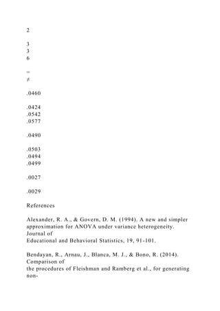
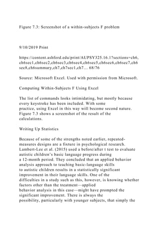
the calculated F value compares to the
critical value from the table.
2. If the F is significant, which groups are significantly
different from each other? That question is
answered by a post hoc test such as Tukey’s HSD.
3. IfF is significant, how important is the result? The question
is answered by an effect-size calculation.
If F is not statistically significant, questions 2 and 3 are
nonissues.
After addressing the first two questions, we now turn our
attention to the
third question, effect size. With the t test in Chapter 5, omega-
squared
answered the question about how important the result was.
There are
similar measures for analysis of variance, and in fact, several
effect-size
statistics have been used to explain the importance of a
significant
ANOVA result. Omega-squared (ω2) and partial eta-squared
(η2) (where
the Greek letter eta [η] is pronounced like “ate a” as in “ate a
grape”) are
both quite common in social-science research literature. Both
effect-size
statistics are demonstrated here, the omega-squared to be
consistent with
Chapter 5, and—because it is easy to calculate and quite
common in the
literature—we will also demonstrate eta-squared. Both statistics
answer
the same question: Because some of the variance in scores is

unexplained,
in other words error variance, how much of the score variance
can be
attributed to the independent variable which, in this recent
example, is the
background environment? The difference between the statistics
is that
omega-squared answers the question for the population of all
such
problems, while the eta-squared result is specific to the
particular data set.
In the social isolation problem, the question was whether
residents of
small towns, suburban areas, and cities differ in their measures
of social
isolation. The respondents’ location is the IV. Eta-squared
estimates how
much of the difference in social isolation is related to where
respondents
live.
The η2 calculation involves only two values, both retrievable
from the
ANOVA table. Formula 6.7 shows the eta-squared calculation:
Formula 6.7
9/10/2019 Print

The formula indicates that eta-squared is the ratio of between-
groups variability to total variability. If there were
no error variance, all variance would be due to the independent
variable, and the sums of squares for between-
groups variability and for total variability would have the same
values; the effect size would be 1.0. With human
subjects, this effect-size result never happens because scores
always fluctuate for reasons other than the IV, but it
is important to know that 1.0 is the upper limit for this effect
size and for omega-squared as well. The lower limit
is 0, of course—none of the variance is explained. But we also
never see eta-squared values of 0 because the
only time the effect size is calculated is when F is significant,
and that can only happen when the effect of the IV
is great enough that the ratio of MSbet to MSwith exceeds the
critical value; some variance will always be
explained.
For the social isolation problem, SSbet = 33.168 and SStot =
41.672, so
According to these data, about 80% of the variance in social
isolation scores relates to whether the respondent
lives in a small town, a suburb, or a city. Note that this amount
of variance is unrealistically high, which can
happen when numbers are contrived.
Omega-squared takes a slightly more conservative approach to
effect sizes and will always have a lower value
than eta-squared. The formula for omega-squared is:
Formula 6.8
Compared to η2, the numerator is reduced by the value of the df
between times MSwith, and the denominator is
increased by the SStot plus MSwith. The error term plays a

more prominent part in this effect size than in η2, thus
the more conservative value. Completing the calculations for ω2
yields the following:
The omega-squared value indicates that about 69% of the
variability in social isolation can be explained by
where the subject lives. This value is 10% less than the eta-
squared value explains. The advantage to using
omega-squared is that the researcher can say, “in all situations
where social isolation is studied as a function of
where the subject lives, the location of the subject’s home will
explain about 69% of the variance.” On the other
hand, when using eta-squared, the researcher is limited to
saying, “in this instance, the location of the subject’s
home explained about 79% of the variance in social isolation.”
Those statements indicate the difference between
being able to generalize compared to being restricted to the
present situation.
Apply It!
Using ANOVA to Test Effectiveness
9/10/2019 Print
Wavebreakmedia Ltd/Wavebreak Media/Thinkstock
A researcher is interested in the relative impact that
tangible reinforcers and verbal reinforcers have on
behavior. The researcher, who describes the study only as
an examination of human behavior, solicits the help of

university students. The researcher makes a series of
presentations on the growth of the psychological sciences
with an invitation to listeners to ask questions or make
comments whenever they wish. The three levels of the
independent variable are as follows:
1. no response to students’ interjections, except to answer
their questions
2. a tangible reinforcer—a small piece of candy—offered after
each comment/question
3. verbal praise offered for each verbal interjection
The volunteers are randomly divided into three groups of eight
each and asked to report for the
presentations, to which students are invited to respond. Note
that there are three independent groups:
Those who participate are members of only one group. The
three options described represent the three
levels of a single independent variable, the presenter’s response
to comments or questions by the
subjects. The dependent variable is the number of interjections
by subjects over the course of the
presentations.
The null hypothesis (H0: µ1 = µ2 = µ3) maintains that response
rates will not vary from group to group,
that in terms of verbal comments, the three groups belong to the
same population. The alternate
hypothesis (HA: not so) maintains that non-random differences
will occur between groups—that, as a
result of the treatment, at least one group will belong to some
other population of responders.
Each subject’s number of responses during the experiment is

indicated in Table 6.10.
Table 6.10: Number of responses given three different levels of
reinforcer
No response Tangible reinforcers Verbal reinforcers
14 18 13
13 15 15
19 16 16
18 18 15
15 17 14
16 13 17
12 17 13
12 18 16
Completing the analysis with Excel yields the following
summary (Table 6.11), with descriptive statistics
first:
Table 6.11: Summary of Excel analysis for the reinforcer study
9/10/2019 Print

Group Count Sum Average Variance
No Response 8 119 14.875 6.982143
Tangible Reinf. 8 132 16.500 3.142857
Verbal Reinf. 8 119 14.875 2.125000
ANOVA
Source of variation SS df MS F P-value Fcrit
Between groups 14.0833333 2 7.041666667 1.72449 0.202565
3.4668
Within groups 85.75 21 4.083333333
With an F = 1.72, results are not statistically significant for a
value less than F0.05 (2,21) = 3.47. The
statistical decision is to “fail to reject” H0. Note that the p
value reported in the results is the probability
that the particular value of F could have occurred by chance. In
this instance, there is a 0.20 probability
(1 chance in 5) that an F value this large (1.72) could occur by
chance in a population of responders. That
p value would need to be p ≤ 0.05 in order for the value of F to
be statistically significant. There are
differences between the groups, certainly, but those differences
are more likely explained by sampling
variability than by the effect of the independent variable.

9/10/2019 Print
6.5 Conditions for the One-Way ANOVA
As we saw with the t tests, any statistical test requires that
certain conditions be met. The conditions might
include characteristics such as the scale of the data, the way the
data are distributed, the relationships between
the groups in the analysis, and so on. In the case of the one-way
ANOVA, the name indicates one of the
conditions. Conditions for the one-way ANOVA include the
following:
The one-way ANOVA test can accommodate just one
independent variable.
That one variable can have any number of categories, but can
have only one IV. In example of rural,
suburban, and city isolation, the IV was the location of the
respondents’ residence. We might have added
more categories, such as rural, semirural, small town, large
town, suburbs of small cities, suburbs of
large cities, and so on (all of which relate to the respondents’
residence) but like the independent t test,
we cannot add another variable, such as the respondents’
gender, in a one-way ANOVA.
The categories of the IV must be independent.
The groups involved must be independent. Those who are
members of one group cannot also be
members of another group involved in the same analysis.
The IV must be nominal scale. Because the IV must be nominal
scale, sometimes data of some other
scale are reduced to categorical data to complete the analysis. If

someone wants to know whether
differences in social isolation are related to age, age must be
changed from ratio to nominal data prior to
the analysis. Rather than using each person’s age in years as the
independent variable, ages are grouped
into categories such as 20s, 30s, and so on. Grouping by
category is not ideal, because by reducing ratio
data to nominal or even ordinal scale, the differences in social
isolation between 20- and 29-year-olds,
for example, are lost.
The DV must be interval or ratio scale. Technically, social
isolation would need to be measured with
something like the number of verbal exchanges that a subject
has daily with neighbors or co-workers,
rather than using a scale of 1–10 to indicate the level of
isolation, which is probably an example of
ordinal data.
The groups in the analysis must be similarly distributed, that is,
showing homogeneity of variance, a
concept discussed in Chapter 5. It means that the groups should
all have reasonably similar standard
deviations, for example.
Finally, using ANOVA assumes that the samples are drawn from
a normally distributed population.
To meet all these conditions may seem difficult. Keep in mind,
however, that normality and homogeneity of
variance in particular represent ideals more than practical
necessities. As it turns out, Fisher’s procedure can
tolerate a certain amount of deviation from these requirements,
which is to say that this test is quite robust. In
extreme cases, for example, when calculated skewness or
kurtosis values reach ±2.0, ANOVA would probably
be inappropriate. Absent that, the researcher can probably
safely proceed.

9/10/2019 Print
6.6 ANOVA and the Independent t Test
The one-way ANOVA and the independent t test share several
assumptions although they employ distinct
statistics—the sums of squares for ANOVA and the standard
error of the difference for the t test, for example.
When two groups are involved, both tests will produce the same
result, however. This consistency can be
illustrated by completing ANOVA and the independent t test for
the same data.
Suppose an industrial psychologist is interested in how people
from two separate divisions of a company differ
in their work habits. The dependent variable is the amount of
work completed after hours at home, per week, for
supervisors in marketing versus supervisors in manufacturing.
The data follow:
Marketing: 3, 4, 5, 7, 7, 9, 11, 12
Manufacturing: 0, 1, 3, 3, 4, 5, 7, 7
Calculating some of the basic statistics yields the results listed
in Table 6.12.
Table 6.12: Statistical results for work habits study
M s SEM SEd MG

Marketing 7.25 3.240 1.146
1.458 5.50
Manufacturing 3.75 2.550 0.901
First, the t test gives
The difference is significant. Those in marketing (M1) take
significantly more work home than those in
manufacturing (M2).
The ANOVA test proceeds as follows:
For all variability from all sources (SStot), verify that the result
of subtracting MG from each score in
both groups, squaring the differences, and summing the squares
= 168:
SStot = ∑(x − MG)2 = 168
For the SSbet, verify that subtracting the grand mean from each
group mean, squaring the difference, and
multiplying each result by the number in the particular group =
49:
SSbet = (Ma − MG)2na + (Mb − MG)2nb = (7.25 − 5.50)2(8) +
(3.75 − 5.50)2(8) = 24.5
For the SSwith, take each group mean from each score in the
group, square the difference, and then sum
the squared differences as follows to verify that SSwith = 119:

9/10/2019 Print
Try It!: #7
What is the relationship between the values of t
and F if both are performed for the same two-
group test?
SSwith = ∑(xa1 − Ma)2 + . . . (xa8 − Ma)2 + ∑(xb1 − Mb)2 . . .
(xb8 − Ma)2 = 119
Table 6.13 summarizes the results.
Table 6.13: ANOVA results for work habit study
Source SS df MS F Fcrit
Total 168 15
Between 49 1 49 5.765 F0.05(1,14) = 4.60
Within 119 14 8.5
Like the t test, ANOVA indicates that the difference
in the amount of work completed at home is
significantly different for the two groups, so at least
both tests draw the same conclusion, statistical
significance. Even so, more is involved than just the
statistical decision to reject H0.
Consider the following:

Note that the calculated value of t = 2.401 and the calculated
value of F = 5.765.
If the value of t is squared, it equals the value of F: 2.4012 =
5.765.
The same is true for the critical values:
T0.05(14) = 2.145, 2.1452 = 4.60
F0.05(1,14) = 4.60
Gosset’s and Fisher’s tests draw exactly equivalent conclusions
when two groups are tested. The ANOVA tends
to be more work, so people ordinarily use the t test for two
groups, but both tests are entirely consistent.
9/10/2019 Print
6.7 The Factorial ANOVA
In the language of statistics, a factor is an independent variable,
and a factorial ANOVA is an ANOVA that
includes multiple IVs. We noted that fluctuations in the DV
scores not explained by the IV emerge as error
variance. In the t-test/ANOVA example above, any differences
in the amount of work taken home not related to
the division between marketing and manufacturing—
differences in workers’ seniority, for example—become
part of SSwith and then the MSwith error. As long as a t test or
a one-way ANOVA is used, the researcher cannot
account for any differences in work taken home that are not

associated with whether the subject is from
marketing or manufacturing, or whatever IV is selected. There
can only be one independent variable.
The factorial ANOVA contains multiple IVs. Each one can
account for its portion of variability in the DV,
thereby reducing what would otherwise become part of the error
variance. As long as the researcher has
measures for each variable, the number of IVs has no theoretical
limit. Each one is treated as we treated the
SSbet: for each IV, a sum-of-squares value is calculated and
divided by its degrees of freedom to produce a mean
square. Each mean square is divided by the same MSwith value
to produce F so that there are separate F values
for each IV.
The associated benefit of adding more IVs to the analysis is that
the researcher can more accurately reflect the
complexity inherent in human behavior. One variable rarely
explains behavior in any comprehensive way.
Including more IVs is often a more informative view of why DV
scores vary. It also usually contributes to a more
powerful test. Recall from Chapter 4 that power refers to the
likelihood of detecting significance. Because
assigning what would otherwise be error variance to the
appropriate IV reduces the error term, factorial
ANOVAs are often more likely to produce significant F values
than one-way ANOVAs; they are often more
powerful tests.
In addition, IVs in combination sometimes affect the DV
differently than they do when they are isolated, a
concept called an interaction. The factorial ANOVA also
calculates F values for these interactions. If a
researcher wanted to examine the impact that marital status and
college graduation have on subjects’ optimism

about the economy, data would be gathered on subjects’ marital
status (married or not married) and their college
education (graduated or did not graduate). Then SS values, MS
values, and F ratios would be calculated for
marital status,
college education, and
the two IVs in combination, the interaction of the factors.
In the manufacturing versus marketing example, perhaps gender
and department interact so that females in
marketing respond differently than females in manufacturing,
for example.
The factorial ANOVA has not been included in this text, but it
is not difficult to understand. The procedures
involved in calculating a factorial ANOVA are more numerous,
but they are not more complicated than the one-
way ANOVA. Excel accommodates ANOVA problems with up
to two independent variables.
9/10/2019 Print
6.8 Writing Up Statistics
Any time a researcher has multiple groups or levels of a
nominal scale variable (ethnic groups, occupation type,
country of origin, preferred language) and the question is about
their differences on some interval or ratio scale
variable (income, aptitude, number of days sober, number of

parking violations), the question can be analyzed
using some form of ANOVA. Because it is a test that provides
tremendous flexibility, it is well represented in
research literature.
To examine whether a language is completely forgotten when
exposure to that language is severed in early
childhood, Bowers, Mattys, and Gage (2009) compared the
performance of subjects with no memory of
exposure to a foreign language in their early childhood to other
subjects with no exposure when the language is
encountered in adulthood. They compared the performance with
phonemes of the forgotten language (the DV) by
those exposed to Hindi (one group of the IV) or Zulu (a second
group of the IV) to the performance of adults of
the same age who had no exposure to either language (a third
group of the IV). They found that those with the
early Hindi or Zulu exposure learned those languages
significantly more quickly as adults.
Butler, Zaromb, Lyle, and Roediger III (2009) used ANOVA to
examine the impact that viewing film clips in
connection with text reading has on student recall of facts when
some of the film facts are inconsistent with text
material. This experiment was a factorial ANOVA with two IVs.
One independent variable had to do with the
mode of presentation including text alone, film alone, film and
text combined. A second IV had to do with
whether students received a general warning, a specific
warning, or no warning that the film might be
inconsistent with some elements of the text. The DV was the
proportion of correct responses students made to
questions about the content. Butler et al. found that learner
recall improved when film and text were combined
and when subjects received specific warnings about possible
misinformation. When the film facts were

inconsistent with the text material, receiving a warning
explained 37% of the variance in the proportion of
correct responses. The type of presentation explained 23% of
the variance.
9/10/2019 Print
Summary and Resources
Chapter Summary
This chapter is the natural extension of Chapters 4 and 5. Like
the z test and the t test, analysis of variance is a
test of significant differences. Also like the z test and t test, the
IV in ANOVA is nominal, and the DV is interval
or ratio. With each procedure—whether z, t, or F—the test
statistic is a ratio of the differences between groups to
the differences within groups (Objective 3).
ANOVA and the earlier procedures, do differ, of course. The
variance statistics are sums of squares and mean
squares values. But perhaps the most important difference is
that ANOVA can accommodate any number of
groups (Objectives 2 and 3). Remember that trying to deal with
multiple groups in a t test introduces the problem
of increasing type I error when repeated analyses with the same
data indicate statistical significance. One-way
ANOVA lifts the limitation of a one-pair-at-a-time comparison
(Objective 1).

The other side of multiple comparisons, however, is the
difficulty of determining which comparisons are
statistically significant when F is significant. This problem is
solved with the post hoc test. This chapter used
Tukey’s HSD (Objective 4). There are other post hoc tests, each
with its strengths and drawbacks, but HSD is
one of the more widely used.
Years ago, the emphasis in scholarly literature was on whether a
result was statistically significant. Today, the
focus is on measuring the effect size of a significant result, a
statistic that in the case of analysis of variance can
indicate how much of the variability in the dependent variable
can be attributed to the effect of the independent
variable. We answered that question with eta squared (η2). But
neither the post hoc test nor eta squared is
relevant if the F is not significant (Objective 5).
The independent t test and the one-way ANOVA both require
that groups be independent. What if they are not?
What if we wish to measure one group twice over time, or
perhaps more than twice? Such dependent group
procedures are the focus of Chapter 7, which will provide an
elaboration of familiar concepts. For this reason,
consider reviewing Chapter 5 and the independent t-test
discussion before starting Chapter 7.
The one-way ANOVA dramatically broadens the kinds of
questions the researcher can ask. The procedures in
Chapter 7 for non-independent groups represent the next
incremental step.
Chapter 6 Flashcards

9/10/2019 Print
Key Terms
analysis of variance (ANOVA)
Name given to Fisher’s test allowing a research study to detect
significant differences among any number of
groups.
error variance
Variability in a measure stemming from a source other than the
variables introduced into the analysis.
eta squared
A measure of effect size for ANOVA. It estimates the amount of
variability in the DV explained by the IV.
factor
An alternate name for an independent variable, particularly in
procedures that involve more than one.
factorial ANOVA
An ANOVA with more than one IV.
F ratio
The test statistic calculated in an analysis of variance problem.
It is the ratio of the variance between the
groups to the variance within the groups.
interaction
Occurs when the combined effect of multiple independent
variables is different than the variables acting

independently.
mean square
Name given to Fisher's test allowing a research study to detect
significant dif‐Click card to see term �
Choose a Study ModeView this study set
https://quizlet.com/
https://quizlet.com/125467580/statistics-for-the-behavioral-
social-sciences-chapter-6-flash-cards/
9/10/2019 Print
The sum of squares divided by the relevant degrees of freedom.
This division allows the mean square to reflect
a mean, or average, amount of variability from a source.
one-way ANOVA
Simplest variance analysis, involving only one independent
variable. Similar to the t test.
post hoc test
A test conducted after a significant ANOVA or some similar
test that identifies which among multiple
possibilities is statistically significant.
sum of squares
The variance measure in analysis of variance. It is the sum of
the squared deviations between a set of scores

and their mean.
sum of squares between
The variability related to the independent variable and any
measurement error that may occur.
sum of squares error
Another name for the sum of squares within because it refers to
the differences after treatment within the same
group, all of which constitute error variance.
sum of squares total
Total variance from all sources.
sum of squares within
Variability stemming from different responses from individuals
in the same group. Because all the individuals
in a particular group receive the same treatment, differences
among them constitute error variance.
Review Questions
Answers to the odd-numbered questions are provided in
Appendix A.
1. Several people selected at random are given a story problem
to solve. They take 3.5, 3.8, 4.2, 4.5, 4.7,
5.3, 6.0, and 7.5 minutes. What is the total sum of squares for
these data?
2. Identify the following symbols and statistics in a one-way
ANOVA:
a. The statistic that indicates the mean amount of difference
between groups.
b. The symbol that indicates the total number of participants.

c. The symbol that indicates the number of groups.
d. The mean amount of uncontrolled variability.
3. A study theorizes that manifested aggression differs by
gender. A researcher finds the following data
from Measuring Expressed Aggression Numbers (MEAN):
Males: 13, 14, 16, 16, 17, 18, 18, 18
Females: 11, 12, 12, 14, 14, 14, 14, 16
Complete the problem as an ANOVA. Is the difference
statistically significant?
4. Complete Question 3 as an independent t test, and
demonstrate the relationship between t2 and F.
9/10/2019 Print
a. Is there an advantage to completing the problem as an
ANOVA?
b. If there were three groups, why not just complete three t tests
to answer questions about
significance?
5. Even with a significant F, a two-group ANOVA never needs a
post hoc test. Why not?
6. A researcher completes an ANOVA in which the number of
years of education completed is analyzed by

ethnic group. If η2 = 0.36, how should that be interpreted?
7. Three groups of clients involved in a program for substance
abuse attend weekly sessions for 8 weeks,
12 weeks, and 16 weeks. The DV is the number of drug-free
days.
8 weeks: 0, 5, 7, 8, 8
12 weeks: 3, 5, 12, 16, 17
16 weeks: 11, 15, 16, 19, 22
a. Is F significant?
b. What is the location of the significant difference?
c. What does the effect size indicate?
8. For Question 7, answer the following:
a. What is the IV?
b. What is the scale of the IV?
c. What is the DV?
d. What is the scale of the DV?
9. For an ANOVA problem, k = 4 and n = 8.
If SSbet = 24.0
and SSwith = 72
a. What is F?
b. Is the result significant?
10. Consider this partially completed ANOVA table:
SS df MS F Fcrit
Between 2

Within 63 3
Total 94
a. What must be the value of N − k?
b. What must be the value of k?
c. What must be the value of N?
d. What must the SSbet be?
e. Determine the MSbet.
f. Determine F.
g. What is Fcrit?
9/10/2019 Print
Answers to Try It! Questions
1. The one in one-way ANOVA refers to the fact that this test
accommodates just one independent
variable. One-way ANOVA contrasts with factorial ANOVA,
which can include any number of IVs.
2. A t test with six groups would need 15 comparisons. The
answer is the number of groups (6) times the
number of groups minus 1 (5), with the product divided by 2: 6
× 5 = 30 / 2 = 15.
3. The only way SS values can be negative is if there has been a
calculation error. Because the values are
all squared values, if they have any value other than 0, they

must be positive.
4. The difference between SStot and SSwith is the SSbet.
5. If F = 4 and MSwith = 2, then MSbet must = 8 because F =
MSbet ÷ MSwith.
6. The answer is neither. If F is not significant, there is no
question of which group is significantly different
from which other group because any variability may be nothing
more than sampling variability. By the
same token, there is no effect to calculate because, as far as we
know, the IV does not have any effect on
the DV.
7. t2 = F
9/10/2019 Print
Chapter Learning Objectives
After reading this chapter, you should be able to do the
following:
1. Explain how initial between-groups differences affect t test
or analysis of variance.
2. Compare the independent t test to the dependent-groups t
test.
3. Complete a dependent-groups t test.

4. Explain what “power” means in statistical testing.
5. Compare the one-way ANOVA to the within-subjects F.
6. Complete a within-subjects F.
7Repeated Measures Designs for IntervalData
Karen Kasmauski/Corbis
9/10/2019 Print
Introduction
Tests of significant difference, such as the t test and analysis of
variance, take two basic forms, depending upon
the independence of the groups. Up to this point, the text has
focused only on independent-groups tests: tests
where those in one group cannot also be subjects in other
groups. However, dependent-groups procedures, in
which the same group is used multiple times, offer some
advantages.
This chapter focuses on the dependent-groups equivalents of the
independent t test and the one-way ANOVA.
Although they answer the same questions as their independent-
groups equivalents (are there significant
differences between groups?), under particular circumstances
these tests can do so more efficiently and with
more statistical power.

9/10/2019 Print
Try It!: #1
If the size of the group affects the size of the
standard deviation, what then is the relationship
between sample size and error in a t test?
7.1 Reconsidering the t and F Ratios
The scores produced in both the independent t and the one-way
ANOVA are ratios. In the case of the t test, the
ratio is the result of dividing the difference between the means
of the groups by the standard error of the
difference:
With ANOVA, the F ratio is the mean square between (MSbet)
divided by the mean square within (MSwith):
With either t or F, the denominator in the ratio reflects how
much scores vary within (rather than between) the
groups of subjects involved in the study. These differences are
easy to see in the way the standard error of the
difference is calculated for a t test. When group sizes are equal,
recall that the formula is
with
and s, of course, a measure of score variation in any group.

So the standard error of the difference is based on the standard
error of the mean, which in turn is based on the
standard deviation. Therefore, score variance within in a t test
has its root in the standard deviation for each
group of scores. If we reverse the order and work from the
standard deviation back to the standard error of the
difference, we note the following:
When scores vary substantially in a group,
the result is a large standard deviation.
When the standard deviation is relatively
large, the standard error of the mean must
likewise be large because the standard
deviation is the numerator in the formula for
SEM.
A large standard error of the mean results in
a large standard error of the difference
because that statistic is the square root of the sum of the
squared standard errors of the mean.
When the standard error of the difference is large, the
difference between the means has to be
correspondingly larger for the result to be statistically
significant. The table of critical values indicates
that no t ratio (the ratio of the differences between the means
and the standard error of the difference)
less than 1.96 to 1 is going to be significant, and even that
value requires an infinite sample size.
Error Variance
9/10/2019 Print

Greg Smith/Corbis
In a study of the impact of substance abuse
programs on addicts’ behavior, confounding
variables could include ethnic background,
age, or social class.
The point of the preceding discussion is that the value of t in
the t test—and for F in an ANOVA—is greatly
affected by the amount of variability within the groups
involved. Other factors being equal, when the variability
within the groups is extensive, the values of t and F are
diminished and less likely to be statistically significant
than when groups have relatively little variability within them.
These differences within groups stem from differences in the
way individuals within the samples react to
whatever treatment is the independent variable; different people
respond differently to the same stimulus. These
differences represent error variance—the outcome whenever
scores differ for reasons not related to the IV.
But within-group differences are not the only source of error
variance in the calculation of t and F. Both t test
and ANOVA assume that the groups involved are equivalent
before the independent variable is introduced. In a t
test where the impact of relaxation therapy on clients’ anxiety is
the issue, the test assumes that before the
therapy is introduced, the treatment group which receives the
therapy and the control group which does not both
begin with equivalent levels of anxiety. That assumption is the
key to attributing any differences after the
treatment to the therapy, the IV.

Confounding Variables
In comparisons like the one studying the effects of relaxation
therapy, the initial equivalence of the groups can be uncertain,
however. What if the groups had differences in anxiety before
the therapy was introduced? The employment circumstances of
each group might differ, and perhaps those threatened with
unemployment are more anxious than the others. What if age-
related differences exist between groups? These other
influences that are not controlled in an experiment are
sometimes called confounding variables.
A psychologist who wants to examine the impact that a
substance abuse program has on addicts’ behavior might set up
a study as follows. Two groups of the same number of addicts
are selected, and one group participates in the substance-abuse
program. After the program, the psychologist measures the
level of substance abuse in both groups to observe any
differences.
The problem is that the presence or absence of the program is
not the only thing that might prompt subjects to
respond differently. Perhaps subjects’ background experiences
are different. Perhaps ethnic-group, age, or social-
class differences play a role. If any of those differences affect
substance-abuse behavior, the researcher can
potentially confuse the influence of those factors with the
impact of the substance-abuse program (the IV). If
those other differences are not controlled and affect the
dependent variable, they contribute to error variance.
Error variance exists any time dependent-variable (DV) scores
fluctuate for reasons unrelated to the IV.
Thus, the variability within groups reflects error variance, and
any difference between groups that is not related

to the IV represents error variance. A statistically significant
result requires that the score variance from the
independent variable be substantially greater than the error
variance. The factor(s) the researcher controls must
contribute more to score values than the factors that remain
uncontrolled.
9/10/2019 Print
Try It!: #2
How does the use of random selection enable us
to control error variance in statistical testing?
Try It!: #3
How do the before/after t test and the matched-
pairs t test differ?
7.2 Dependent-Groups Designs
Ideally, any before-the-treatment differences between the
groups in a study will be minimal. Recall that random
selection entails every member of a population having an equal
chance of being selected. The logic behind
random selection dictates that when groups are randomly drawn
from the same population, they will differ only
by chance; as sample size increases, probabilities suggest that
they become increasingly similar in characteristic
to the population. No sample, however, can represent the

population with complete fidelity, and sometimes the
chance differences affect the way subjects respond to the IV.
One way researchers reduce error variance is to adopt
what are called dependent-groups designs. The
independent t test and the one-way ANOVA required
independent groups. Members of one group could not
also be members of other groups in the same study.
But in the case of the t test, if the same group is
measured, exposed to a treatment, and then measured
again, the study controls an important source of error
variance. Using the same group twice makes the initial
equivalence of the two groups no longer a concern. Other
aspects being equal, any score difference between the first and
second measure should indicate only the impact
of the independent variable.
The Dependent-Samples t Tests
One dependent-groups test where the same group is measured
twice is called the before/after t test. An
alternative is called the matched-pairs t test, where each
participant in the first group is matched to someone in
the second group who has a similar characteristic. The
before/after t test and the matched-pairs t test both have
the same objective—to control the error variance that is due to
initial between-groups differences. Following are
examples of each test.
The before/after design: A researcher is interested in the impact
that positive reinforcement has on
employees’ sales productivity. Besides the sales commission,
the researcher introduces a rewards
program that can result in increased vacation time. The
researcher gauges sales productivity for a
month, introduces the rewards program, and gauges sales

productivity during the second month for the
same people.
The matched-pairs design: A school counselor is interested in
the impact that verbal reinforcement has
on students’ reading achievement. To eliminate between-groups
differences, the researcher selects 30
people for the treatment group and matches each person in the
treatment group to someone in a control
group who has a similar reading score on a standardized test.
The researcher then introduces the verbal
reinforcement program to those in the treatment group for a
specified period of time and then compares
the performance of students in the two groups.
Although the two tests are set up differently, both
calculate the t statistic the same way. The differences
between the two approaches are conceptual, not
mathematical. They have the same purpose—to
control between-groups score variation stemming
from nonrelevant factors.
9/10/2019 Print
Calculating t in a Dependent-Groups Design
The dependent-groups t may be calculated using several
methods. Each method takes into account the
relationship between the two sets of scores. One approach is to
calculate the correlation between the two sets of
scores and then to use the strength of the correlation as a

mechanism for determining between-groups error
variance: the higher the correlation between the two sets of
scores, the lower the error variance. Because this text
has yet to discuss correlation, for now we will use a t statistic
that employs “difference scores.” The different
approaches yield the same answer.
The distribution of difference scores came up in Chapter 5 when
it introduced the independent t test. Recall that
the point of that distribution is to determine the point at which
the difference between a pair of sample means
(M1 − M2) is so great that the most probable explanation is that
the samples came from different populations.
Dependent-groups tests use that same distribution, but rather
than the difference between the means of the two
groups (M1 − M2), the numerator in the t ratio is the mean of
the differences between each pair of scores. If that
mean is sufficiently different from the mean of the population
of difference scores (which, recall, is 0), the t
value is statistically significant; the first set of measures
belongs to a different population than the second set of
measures. That may seem odd since in a before/after test, both
sets of measures come from the same subjects,
but the explanation is that those subjects’ responses (the DV)
were altered by the impact of the independent
variable; their responses are now different.
The denominator in the t ratio is another standard error of the
mean value, but in this case, it is the standard error
of the mean of the difference scores. The researcher checks for
significance using the same criteria as for the
independent t:
A critical value from the t table, determined by degrees of
freedom, defines the point at which the

calculated t value is statistically significant.
The degrees of freedom are the number of pairs of scores minus
1 (n − 1).
The dependent-groups t test statistic uses this formula:
Formula 7.1
where
Md = the mean of the difference scores
SEMd = the standard error of the mean for the difference scores
The steps for completing the test are as follows:
1. From the two scores for each subject, subtract the second
from the first to determine the difference
score, d, for each pair.
2. Determine the mean of the d scores:
9/10/2019 Print
3. Calculate the standard deviation of the d values, sd.
4. Calculate the standard error of the mean for the difference
scores, SEMd, by dividing sd by the square
root of the number of pairs of scores,

5. Divide Md by SEMd, the standard error of the mean for the
difference scores:
Figure 7.1 depicts these steps.
The following is an example of a dependent-measures t test: A
psychologist
is investigating the impact that verbal reinforcement has on the
number of
questions university students ask in a seminar. Ten upper-level
students
participate in two seminars where a presentation is followed by
students’
questions. In the first seminar, the instructor provides no
feedback after a
student asks the presenter a question. In the second seminar, the
instructor
offers feedback—such as “That’s an excellent question” or
“Very interesting
question” or “Yes, that had occurred to me as well”—after each
question.
Is there a significant difference between the number of
questions students
ask in the first seminar compared to the number of questions
students ask in
the second seminar? Problem 7.1 shows the number of questions
asked by
each student in both seminars and the solution to the problem.
Problem 7.1: Calculating the before/after t test
Seminar 1 Seminar 2 d
1 1 3 −2

2 0 2 −2
Figure 7.1: Steps for
calculating the before/after t
test
9/10/2019 Print
Seminar 1 Seminar 2 d
3 3 4 −1
4 0 0 0
5 2 3 −1
6 1 1 0
7 3 5 −2
8 2 4 −2
9 1 3 −2
10 2 1 1
∑d = −11
1. Determine the difference between each pair of scores, d,
using subtraction.

2. Determine the mean of the difference, the d values (Md).
3. Calculate the standard deviation of the d values (Sd). Verify
that
Sd = 1.101.
4. Just as the standard error of the mean in the earlier test was
s√n, determine standard error of the
mean for the difference scores (SEMd) by dividing the result of
step 3 by the square root of the
number of pairs. Verify that
5. Divide Md by SEMd to determine t.
6. As noted earlier, the degrees of freedom for the critical value
of t for this test are the number of
pairs of scores, np − 1.
t0.05(9) = 2.262
The calculated value of t exceeds the critical value from Table
5.1 (Table B.2 in Appendix B). Therefore, the
result is statistically significant. Note that we are interested in
the absolute value of the calculated t. Because the
question was whether there is a significant difference in the
number of questions, it is a two-tailed test. It does
not matter which session had the greater number—whether
Session 1 is larger than Session 2 or the other way
9/10/2019 Print

Try It!: #4
What does it mean to say that the within-subjects
test has more power than the independent t test?
around. The students in the second session, where questions
were followed by feedback, asked significantly
more questions than the students in the first session, when no
feedback was offered by the instructor.
Degrees of Freedom, the Dependent-Groups Test, and Power
When Md = −1.1, the two sets of scores show comparatively
little difference. What makes such a small mean
difference statistically significant? The answer is in the amount
of error variance in this problem. When there is
minimal error variance—for example, the standard error of the
difference scores is just 0.348—comparatively
small mean differences can be statistically significant. The
ability to detect such small differences, which are
nevertheless statistically significant, is the rationale for using
dependent-groups tests, which brings us back to
power in statistical testing, a topic first raised in Chapter 6.
Table B.2 in Appendix B, the critical values of t, indicates that
critical values decline as degrees of freedom
increase. That occurs not only in the critical values for t, but
also for F in analysis of variance and, in fact, for
most tables of critical values for statistical tests.
For the dependent-groups t test, the degrees of freedom are the
number of pairs of related scores, −1.
For the independent-groups t test (Chapter 5),

df = n1 + n2 −2
With the smaller numerical value for df, the
dependent-groups test has the higher standard to meet
for statistical significance, even though the number of
raw scores is the same. But even a test with a larger
critical value can produce significant results when it
has less error variance. This is what dependent-
groups tests do. The central point is that when each
pair of scores comes from the same participant, or
from a matched pair of participants, the random
variability from nonequivalent groups is minimal
because scores tend to vary similarly for each pair, resulting in
relatively little error variance. The reduced error
more than compensates for the fewer degrees of freedom and the
associated larger critical value.
Recall that in statistical testing, power is defined as the
likelihood of detecting a significant difference when it is
present. The more powerful statistical test is the one that will
most readily detect a significant difference. As long
as the sets of scores are closely related, the dependent-
measures, or dependent-groups, test is more powerful than
the independent-groups equivalent.
A Matched-Pairs Example
The other form of the dependent-groups t test is the matched-
pairs design. In this approach, rather than measure
the same people repeatedly, each participant in one group is
paired with a participant who is similar from the
other group.
For example, consider a psychologist who wants to determine

whether a video on domestic violence will prompt
viewers to be less tolerant of domestic violence. The
psychologist selects a group of subjects, introduces them to
the video which they view, and measures their attitudes toward
domestic violence. A second group does not view
the video. Reasoning that age and gender might be relevant to
attitudes about domestic violence, the
9/10/2019 Print
psychologist selects people for the second group who match
these characteristics of those in the first group.
Problem 7.2 shows subjects’ scores from an instrument designed
to measure attitudes about domestic violence
and the matched-pairs t solution.
Problem 7.2: Calculating a matched-pairs t test
Subject Viewed Did not view d
1 1.5 3 −1.5
2 4 0 4
3 3 2 1
4 0 0 0
5 2 0 2

6 4.5 4 0.5
7 6 2 4
8 0 1 −1.0
9 5.25 2 3.25
10 2 3 −1.0
Verify that Md = 1.125
The absolute value of t is less than the critical value from Table
5.1 (or Table B.2 in Appendix B) for df = 9. The
difference is not statistically significant. There are probably
several ways to explain the outcome, but we will
explore just three.
1. The most obvious explanation is that the video was
ineffective. Subjects’ attitudes were not significantly
altered as a result of the viewing.
2. Another explanation has to do with the matching. Perhaps age
and gender are not related to individuals’
attitudes. Prior experience with domestic violence may be the
most important characteristic, a factor left
uncontrolled in the pairing.
3. Another explanation is related to sample size. Small samples
tend to be more variable than larger
samples, and variability is what the denominator in the t ratio
reflects. Perhaps if this had been a larger
sample, the SEMd would have had a smaller value and the t
would have been significant.
The second explanation points out the disadvantage of matched-

pairs designs compared to repeated-measures
designs. The individual conducting the study must be in a
position to know which characteristics of the
9/10/2019 Print
participants are most relevant to explaining the dependent
variable so that they can be matched in both groups.
Otherwise it is impossible to know whether a nonsignificant
outcome reflects an inadequate match, control of the
wrong variables, or a treatment that just does not affect the DV.
Comparing the Dependent-Samples t Test to the Independent t
Test
To compare the dependent-samples t test and the independent t
more directly, we will apply both tests to the
same data to illustrate how each test deals with error variance.
Before beginning, a necessary caution: Once data
are collected, there is no situation where someone can choose
which test to use. Either the groups are
independent, or they are not. Our comparison is purely an
academic exercise.
A university program encourages students to take a service-
learning class that emphasizes the importance of
community service as a part of the students’ educational
experience. Data are gathered on the number of hours
former students spend in community service per month after
they complete the course and graduate from the

university.
For the independent t test, the students are divided between
those who took a service-learning class and
graduates of the same year who did not.
For the dependent-groups t test, those who took the service-
learning class are matched to a student with
the same major, age, and gender who did not take the class.
The data and the solutions to both tests are listed in Problem
7.3.
Problem 7.3: The before/after t versus the independent t test
Student Class No class d
1 4 3 1
2 3 2 1
3 3 2 1
4 2 2 0
5 3 2.5 0.5
6 4 3 1
7 1 2 −1
8 5 4 1
9 6 5 1
10 4 3 1

M 3.50 2.850 0.650
s 1.434 1.001 0.669
SEM 0.453 0.316 0.211
9/10/2019 Print
For an independent t test, the results show:
The result is not significant.
For a matched-pairs t test, the results show:
The result is significant.
Because the differences between the scores are quite consistent,
as they tend to be when participants are matched
effectively, very little variation exists between the individuals
in each pair. Minimal variation results in a
comparatively small standard deviation of difference scores and
a small standard error of the mean for the
difference scores. The small standard deviation and standard
error of the mean make it more likely that t ratios
with even relatively small numerators will be statistically
significant. Since the independent t test does not
assume that the two groups are related, error variance is based
on the differences within the groups of raw scores,
rather than between the individuals in each pair, and the
denominator is large enough that in that test, the t value

is not significant.
Computing the Dependent-Groups t Test Using Excel
To use Excel to complete Problem 7.3 as a dependent-groups
test, follow this procedure:
1. Create the data file in Excel.
2. a. Label Column A “Class” to indicate those who had the
service learning class, and label column
B “No Class.”
b. Enter the data, beginning with cell A2 for the first group and
cell B2 for the second group.
3. Click the Data tab at the top of the page.
4. At the extreme right, choose Data Analysis.
5. In the Analysis Tools window, select ttest: Paired Two
Sample for Means and click OK.
6. In the blanks for Variable 1 Range and Variable 2 Range,
enter A2:A11 for the data in the first (Class)
group (cells A2 to A11), and enter B2:B11 for the No Class data
(cells B2 to B11).
7. Indicate that the hypothesized mean difference is 0. This
reflects the value for the mean of the
distribution of difference scores.
8. Indicate A13 for the output range so that the results do not
overlay the data scores.
9. Click OK.
Widen column A so that all the output is readable. Figure 7.2
shows the resulting screenshot.

9/10/2019 Print
In the Excel solution, t = 3.074 rather than the 3.081 from the
manually calculated solution. Excel calculates the
correlation between scores to find a solution, rather than
determining the difference between scores as we did. In
any event, the very minor difference, 0.007, between the
solution shown in Problem 7.3 and the Excel solution in
Figure 7.2 is not relevant to the outcome. The Excel output also
indicates results for one-tailed and two-tailed
tests. At p = 0.05, the outcome is statistically significant in
either case.
Figure 7.2: Excel output for the dependent-
samples t test using data from Problem 7.3
Comparing the Two Dependent t Tests
The before/after and matched-pairs approaches to calculating a
dependent-groups t test have their individual
advantages. The before/after design provides the greatest
control over the extraneous variables that can confound
the results in a matched-pairs design. The matching approach
always has the chance that subjects in Group 2 are
not matched closely enough on some relevant variable to
minimize the error variance. In the service-learning
example, students were matched according to age, major, and
gender. But if marital status affects students’

willingness to be involved in community service and that
variable is not controlled, an imbalance of married/not-
married students could confound results. The before/after
procedure involves the same subjects, and unless their
status on some important variable changes between measures (a
rash of marriages between the first and second
measurement, for example), that approach will better control
error variance.
Note that the matched-pairs approach relies on a large sample
from which to draw to select participants who
match those in the first group. As the number of variables on
which participants must be matched increases, so
must the size of the sample from which to draw to find
participants with the correct combination of
characteristics.
9/10/2019 Print
mbot/iStock/Thinkstock
Apply It!
Repeated Measures
A research team is investigating the impact of fixed-ratio
reinforcement on laboratory rats. Initially, the rats receive
food reinforcers each time they make a correct turn in a
maze. The control rats receive no reinforcement. The
dependent variable is the amount of time in seconds it
takes each rat to complete the maze. Table 7.1 shows the

results of the investigation.
Table 7.1: Impact of fixed-ratio reinforcement on laboratory
rats
Rat
Time(s)
With reinforcement Without reinforcement
A 112 120
B 85 82
C 103 116
D 154 168
E 65 75
F 52 51
G 85 96
H 72 79
I 167 178
J 123 141
K 142 153
Table 7.2 shows the Excel solution to the t test.
Table 7.2: Summary statistics from the Excel t test

Variable 1 Variable 2
Mean 105.45 114.45
Variance 1428.67 1736.27
Observations 10 10
Pearson Correlation 0.99
Hypothesized Mean Difference 0.00
df 9
9/10/2019 Print
Variable 1 Variable 2
t Stat −4.817
P(T←t) one-tail 0.0003
t Critical one-tail 1.8331
P(T←t) two-tail 0.0007
t Critical two-tail 2.2622
The magnitude of the calculated value of t = −4.817 exceeds the

critical two-tail value from the table of
tcrit = 2.26. The result indicates that providing reinforcement
for correct decisions has a statistically
significant effect on the time it takes a rat to complete the
maze.
The advantage of the matched-pairs design, on the other hand,
is that it takes less time to execute. The treatment
group and the control group can both be involved in the study at
the same time. By way of a summary, note the
comparisons among t tests in Table 7.3.
Table 7.3: Comparing the t tests
Independent t Before/after Matched-pairs
Groups Independent groups One group
measured twice
Two groups: each subject from the first
group matched to one in the second
Denominator/error
term
Within-groups and
between-groups
variability
Within-groups
variability only
Within-groups variability only

9/10/2019 Print
7.3 The Within-Subjects F
Sometimes two measures of the same group are not enough to
track changes in the dependent variable. Maybe
the researchers conducting the service-learning study want to
compare how much time students devoted to
community service the year they graduated, one year later, and
then two years after graduation. The within-
subjects F is a dependent-groups procedure for two or more
groups of scores when the DV is interval or ratio
scale. Because the dependent-groups t test is the repeated-
measures equivalent of the independent t test, the
within-subjects F is the repeated-measures or matched-pairs
equivalent of the one-way ANOVA. The same
Ronald Fisher who developed analysis of variance also
developed this test, which is a form of ANOVA, and the
test statistic is still F.
Here too, the dependent groups can be formed either by
repeatedly measuring the same group or by matching
separate groups of participants on the relevant variables. When
more than two groups are involved, matching
becomes increasingly problematic, however. Although it is
theoretically possible to match the participants across
any number of groups, to match more than one or two relevant
variables across more than two or three groups of
subjects is a highly complex undertaking. Imagine the
difficulty, for example, of matching subjects on some

measure of aptitude, their income, and their level of optimism
in three or more different groups. Even matching
these variables for two groups might prove quite difficult. For
this reason, repeatedly measuring the same
participants is much more common than matching across several
groups.
Managing Error Variance in the Within-Subjects F
Recall from Chapter 6 that when Fisher developed ANOVA, he
shifted away from calculating score variability
with the standard deviation, standard error of the mean, and so
on and used sums of squares instead. The
particular sums of squares computed are the key to the strength
of this procedure.
If a researcher measures a group of participants in a study on a
dependent variable at three different intervals and
records their scores in parallel columns, the result is a data
sheet similar to Table 7.4.
The column scores for the first, second, and third measures are
treated the way scores from three
different groups were treated in a one-way ANOVA; the
differences from column to column reflect the
effect of the IV, the treatment.
The participant-to-participant differences, which are like the
within-group differences in a one-way
ANOVA, are reflected in the differences in the scores from row
to row. Those differences are error
variance, just as they were in the one-way ANOVA.
Table 7.4: A data sheet
1st measure 2nd measure 3rd measure

Participant 1 . . .
Participant 2 . . .
The within-subjects F calculates the variability between rows
(the within-groups variance), and then,
because that variance comes from participant-to- participant
differences that will be the same in each
group, eliminates it from further analysis.
The only error variance that remains is that which does not stem
from initial person-to-person
differences. It will be from such sources as inaccurate measures
of the DV, mistakes in coding the DV,
or differences in how sensitive the subjects are to the DV that
change from treatment to treatment.
9/10/2019 Print
In the dependent-samples t test, the within-subjects variance—
error variance—is reduced by using subjects in
two groups that are highly similar to begin with or because they
are the same people measured before and after a
treatment. In either case, initial between-groups differences, an
important source of variance, are minimized, and
attributing differences to the effect of the independent variable
becomes easier.
In the within-subjects F, the variability within groups is
calculated and then simply discarded so that it is no
longer a part of the analysis. That cannot be done in the one-

way ANOVA because the amount of variability
within groups is different for each group, and there is no way to
separate it from the balance of the error variance
in the problem.
A Within-Subjects F Example
A psychologist is studying practice effect in connection with the
ability of 12-year-olds to solve a series of
puzzles involving logic and reasoning. The study has five
subjects, who solve as many puzzles as they can
during a 30-minute period. The psychologist conducts three
trials an hour apart. Although the puzzles are similar,
each trial involves different puzzles. The researcher wants to
answer the question whether greater familiarity
with the puzzles is associated with solving more puzzles
correctly. Table 7.5 shows the study’s results.
Table 7.5 Data from puzzle-solving study
Number of puzzles solved
1st trial 2nd trial 3rd trial
Diego 2 5 4
Harold 4 7 7
Wilma 3 6 5
Carol 4 5 6
Moua 5 8 9
The independent variable (the IV, the treatment) is the
particular trial. The dependent variable (the DV) is the

number of puzzles successfully solved. The research question is
whether the second or third trials will result in
significantly more puzzles solved than in the first trial. In
Chapter 6, the sum of squares between (SSbet)
measured the variability related to the IV. This study gauges the
same source of variance, except that it is called
the sum of squares between columns (SScol).
The Components of the Within-Subjects F
Calculating the within-subjects F begins just as the one-way
ANOVA begins, by determining all variability from
all sources with the sum of squares total (SStot). It is calculated
the same way as it was in Chapter 6:
1. The formula for the sum of squares total is
SStot =∑(x − MG)2
a. Subtract each score (x) from the mean of all the scores from
all the groups (MG),
b. square the difference, and then
c. sum the squared differences.
9/10/2019 Print
The balance of the problem is completed with the following
steps:
2. The equation for the sum of squares between columns (SScol)

is much like SSbet in the one-way
ANOVA. The scores in each column are treated the same way
the different groups were treated in the
one-way ANOVA. For columns 1, 2, and through k:
Formula 7.2
SScol = (Mcol 1 − MG)2ncol 1 + (Mcol 2 − MG)2ncol 2 + . . . +
(Mcol k − MG)2ncol k
a. calculate the mean for each column of scores (Mcol),
b. subtract the mean for all the data (MG) from each column
mean,
c. square the result, and
d. multiply the squared result by the number of scores in the
column (ncol).
3. The sum of squares between rows is also like the SSbet from
the one-way problem except that it treats
the scores for each row as a separate group. For rows 1, 2, and
through i:
Formula 7.3
SSrows = (Mrow 1 − MG)2nrow 1 + (Mrow 2 − MG)2nrow 2 + .
. . + (Mrow i − MG)2nrow i
a. calculate the mean for each row of scores (Mrow),
b. subtract the mean for all the data (MG) from each row mean,
c. square the result, and
d. multiply the squared result by the number of scores in the
row.
4. The residual sum of squares is the error term in the within-
subjects F. It is the equivalent of SSwith or
the SSerr in the one-way ANOVA. With the within-subjects F,

the person-to-person differences within
each measure are calculated and eliminated since they are the
same for each set of measures.
Unexplained variance is what remains after the treatment effect
(the effect of the IV) and the person-to-
person differences within in each group are eliminated:
Formula 7.4
SSresid = SStot − SScol − SSrows
a. If from all variance from all sources (SStot),
b. the treatment effect (SScol) is subtracted
c. and the person-to-person differences (SSrows) are subtracted,
d. what remains is unexplained variance, error.
Completing the Within-Subjects F Calculations
Just as with one-way problems, the mean square values are
calculated by dividing the sums of squares by their
degrees of freedom. The degrees of freedom values are as
follows:
df total = N − 1
9/10/2019 Print
df columns = number of columns − 1
df rows = number of rows − 1
df residual = df columns × df rows

Although we listed the degrees of freedom values for total and
rows, as well as for columns and residuals, there
are no MS values for total and rows. The df values for those two
variance measures are listed because the sum of
all df values must equal df for total; they allow for a quick
check of df values. The next step is to complete the
ANOVA table, including the calculation of F. We can determine
the test statistic, F, in the within-subjects
ANOVA by dividing the treatment effect (MScol) by the error
term (MSresid); F = MScol / MSresid
Problem 7.4 shows the calculations and the table for the impact
of the practice-effects study.
As with one-way ANOVA, the first step is to calculate the
SStot. It is the sum of the squared differences between
each individual score (x) and the grand mean (MG). The SStot
is followed by the SS for the differences between
columns (SScol). It is the sum of the squared differences
between each column mean (Mcol1, for example) and the
grand mean (MG), times the number of scores in the column
(ncol1, for example). Next, calculate the SS for the
differences from row to row. For each row, square the
difference between the row mean (Mr1, for example) and
the grand mean (MG), and then multiply the squared difference
by the number of scores in the row (nr1, for
example). Finally, find the error term—the residual sum of
squares—which is what remains from SStot − SScol −
SSrows.
Problem 7.4: A within-subjects F example
Puzzles completed
1st trial 2nd trial 3rd trial Row means

Diego 2 5 4 3.667
Harold 4 7 7 6.0
Wilma 3 6 5 4.667
Carol 4 5 6 5.0
Moua 5 8 9 7.333
Column means 3.60 6.20 6.20
Grand mean (Md) 5.333
1. SStot = ∑(x − MG)2
(2 − 5.333)2 + (4 − 5.333)2 + . . . + (9 − 5.333)2 = 49.333
2. SScol = (Mcol 1 – MG)2ncol 1 + (Mcol 2 – MG)2ncol 2 + . .
. + (Mcol k – MG)2ncol k
(3.6 − 5.333)25 + (6.2 − 5.333)25 + (6.2 − 5.333)25 = 22.533
9/10/2019 Print
Try It!: #5
How is the error term in the within-subjects F
different from that in the one-way ANOVA?

3. SSrows = (Mr1 – MG)2nr1 + (Mr2 – MG)2nr2 + . . . + (Mri –
MG)2nri
(3.667 − 5.333)23 + (6.0 − 5.333)23 + (4.667 − 5.333)23 + (5.0
− 5.333)23 + (7.333 − 5.333)23 =
23.333
4. The residual sum of squares.
SSresid = SStot − SScol − SSrows = 49.333 − 22.533 − 23.333
= 3.467
The ANOVA table
Total 49.333 14
Columns 22.533 2 11.267 26.0 4.46
Rows 23.333 4
Residual 3.467 8 0.433
The calculated value of F exceeds the critical value of F from
the table. The number of puzzles completed is
significantly different for the different trials. The significant F
indicates that differences of this magnitude are
unlikely to have occurred by chance.
Completing the Post Hoc Test
Ordinarily, the calculation of F leaves unanswered the question
of which set of measures is significantly different
from which. However, in this particular problem there is only

one possibility. Because both the second trial and
the third trial measures have the same mean (M = 6.20), they
must both be significantly different from the only
other group of measures in the problem, the first trial measures,
for which M = 3.6. As a demonstration of how
we would determine which groups were significantly different
from which were it otherwise, honestly significant
difference (HSD) is completed anyway.
The HSD procedure is the same as for the one-way
test, except that the error term is now MSresid.
Substituting MSresid for MSwith in the formula
provides
where x is a value from Table B.4 in Appendix B. It is based on
the number of means, which is the same as the
number of groups of measures, 3 in the example, and the df for
MSresid, which is 8. n = the number of scores in
any one measure, 5 in this instance.
For the number-of-puzzles-solved correctly study,
9/10/2019 Print
A difference of 0.306 or greater between any pair of means is
Using the same approach used in Chapter 6, the matrix in Table
7.6 indicates how the difference between each
pair of means helps us determine which differences are

Table 7.6: Matrix of differences of means
1st trial (3.6) 2nd trial (6.2) 3rd trial (6.2)
1st trial (3.6) diff = 0 diff = 2.6* diff = 2.6*
2nd trial (6.2) diff = 0.00
3rd trial (6.2)
*Indicates a significant difference
The first trial measures are significantly different from the
second and third measures. Because the mean values
for the second and third trial measures are the same, neither of
those two is significantly different from the other.
For these 12-year-old subjects working with this kind of
logic/reasoning puzzle, practice effect is greatest from
first to subsequent trials.
Calculating the Effect Size
The final question for a significant F is the question of the
practical importance of the result. Using eta-squared
as the measure of effect size produces the following:
with SScol taking the place of SSbet in the one-way ANOVA.
For the problem just completed, SScol = 22.533 and SStot =
49.333, so
The eta-squared value indicates that approximately 46% of the
variance in the number of puzzles solved
successfully by these subjects can be explained by whether it

was the first or some subsequent trial.
Apply It!
The Meditation Pilot Program Revisited
Recall Chapter 5’s example of the middle school that adopted a
meditation program in an effort to relieve
stress among students, increase their test scores, and improve
student behavior. In the earlier chapter, we
used a one-sample t test to determine that a statistically
significant increase in GPAs occurred among
9/10/2019 Print
participating students. Now, we will use a within-subject F test
to see if their stress levels have decreased
over successive intervals.
Ten randomly chosen students selected for the program filled
out questionnaires about their stress levels.
Scores ranged from 1 to 10, with 10 indicating the most stress.
The survey was given before the start of
the program and at three-month intervals. The time elapsed
represents the independent variable, the
treatment effect that drives this analysis. The dependent
variable is the stress score. This example
includes four groups of DV scores.
Results of the stress questionnaires appear in Table 7.7.

Table 7.7: Stress over time for 10 students
Student
Time (months)
0 3 6 9
1 7 6 6 6
2 9 6 5 5
3 7 5 5 4
4 5 3 3 2
5 7 6 4 4
6 8 5 7 5
7 5 4 4 3
8 7 5 6 5
9 6 6 4 4
10 7 5 5 5
Table 7.8 shows results of the within-subject F test calculations.
Table 7.8: Within-subject F test calculations for changes in
stress over time
Source SS df MS F
Total 82.000 39

Columns 34.475 3 11.492 26.36
Subjects 35.725 9
Residual 11.775 27 0.436
f.05(3,27) 2.96
The F value of 26.36 is greater than the critical F value of 2.96,
results that are unlikely to have occurred
by chance. It seems clear that the length of time during which
students practice meditation has a
significant effect on stress levels.
The significant value of F indicates the need for a post hoc test
to determine which group(s) of stress
measures are significantly different from which others. Recall
that the HSD formula is as follows:
9/10/2019 Print
Entering the MSresid value from the ANOVA table and relevant
value of x from the Tukey’s table gives us
A difference of 0.81 or greater between any two means indicates
that the difference between those
intervals is statistically significant. A matrix that shows the
difference between each pair of means makes
interpreting the HSD value easier, as in Table 7.9.

Table 7.9: Detecting significant differences among multiple
groups
0 month (6.8) 3 months (5.1) 6 months (4.9) 9 months (4.3)
0 month (6.8) diff = 1.7* diff = 1.9* diff = 2.5*
3 months (5.1) diff = 0.2 diff = 0.8
6 months (4.9) diff = 0.6
9 months (4.3)
*Indicates a significant difference
Comparing the means reveals that the greatest decrease in stress
occurs during the first three months of
the meditation program, a difference between the means of 1.7.
It is also apparent that the stress scores
for any interval are significantly different from the stress
recorded before the experiment began.
To determine the practical importance of the decline in stress
measures requires an effect-size calculation.
Once again, we will use eta squared. For the problem just
completed, Icol = 34.475, and SStot = 82.000.
Therefore,
About 42% of the variance in stress can be explained by how
long the student has been enrolled in the
meditation program.
The within-subjects F test allowed analysis of students’ stress
levels at multiple times throughout the year
and showed that the program was reducing stress levels by

significant amounts from the stress recorded
among subjects before the program began.
Comparing the Within-Subjects F and the One-Way ANOVA
In the one-way ANOVA, within-group variance is different for
each group because each group is made up of
different participants. With no way to distinguish between the
subject-to- subject variability within groups from
other sources of error variance, the subject-to-subject variance
cannot be calculated and eliminated from further
9/10/2019 Print
analysis, as it can be in the within-subjects F. The smaller error
term that is the result in the within-subjects test
(which, remember, is the divisor in the F ratio) allows relatively
small differences between sets of measures to be
The effect of eliminating some sources of error is illustrated by
using the same data in the study of practice effect
on problem solving. If those same data were treated as the
number of problems solved by separate groups, rather
than by the same group over time, the researcher analyzes using
a one-way ANOVA instead of the within-
subjects F. We caution that this approach is for illustration only
because groups are either independent or

dependent, and one set of data cannot fit both scenarios. We use
it here to allow us to compare the error terms for
each approach.
The SStot and the SSbet will be the same as the SStot and the
SScol in the within-subjects problem.
SStot = 49.333
SSbet = 22.533
But with no way to isolate the participant-to-participant
differences from the balance of the error variance in the
one-way ANOVA, the SSwith amount in a one-way ANOVA
ends up the same as SSrows + SSresid in the within-
subjects F in Problem 7.4.
SSwith = ∑(xa − Ma)2 + ∑(xb − Mb)2 + ∑(xc − Mc)2 = (2 −
3.60)2 + (4 − 3.60)2 + . . . + (9 − 6.20)2 =
26.80
From Table 7.10, we can make the following observations:
The number of degrees of freedom for “within” changes from
the 8 for residual to 12, which results in a
smaller critical value for the independent-groups test, but that
adjustment does not compensate for the
additional error in the term.
Table 7.10: The within-subjects F example repeated as a one-
way ANOVA
The ANOVA table

Total 49.333 14
Between 22.533 2 11.267 5.045 3.89
Within 26.800 12 2.233
Note that the sum of squares for the error term jumps from
3.467 in the within- subjects test to 26.80 in
the independent-groups test.
The F value is reduced from 26.0 in the within problem to 5.046
in the one-way problem, a factor of
about one-fifth.
Although calculating both one-way ANOVA and with-subjects F
results for the same data is not realistic, the
comparison illustrates what can be gained by setting up a
dependent-groups test. That is an option that
researchers do have at the planning level.
Another Within-Subjects F Example
9/10/2019 Print
Try It!: #6
How do the eta squared values compare for the
one-way ANOVA/within-subjects F problem?
A psychologist working at a federal prison is interested in the
relationship between the amount of time a prisoner

is incarcerated and the number of violent acts in which the
prisoner is involved. Using self-reported data, inmates
respond anonymously to a questionnaire administered one
month, three months, six months, and nine months
after incarceration. Problem 7.5 shows the data and the solution.
The results (F) indicate that there are significant
differences in the number of violent acts documented
for the inmate related to the length of time the inmate
has been incarcerated. The HSD results indicate that
those incarcerated for one month are involved in a
significantly different number of violent acts than
those who have been in for three or six months.
Those who have been in for six months are involved
in a significantly different number of violent acts than
those who have been in for nine months. The eta
squared value indicates that about 37% of the variance in
number of violent acts is a function of how long the
inmate has been incarcerated.
Problem 7.5: Another within-subjects F example: Violent acts
and time of
incarceration
Percentile improvement
Inmate 1 month 3 months 6 months 9 months Row means
1 4 3 2 5 3.50
2 5 4 3 4 4.0
3 3 1 1 2 1.750
4 4 2 1 3 2.50

5 2 1 2 3 2.0
Column means 3.60 2.20 1.80 3.40
MG = 2.750
Verify that
1. SStot = ∑(x − MG)2 = 31.750
2. SScol = (Mcol 1 − MG)2ncol 1 + (Mcol 2 − MG)2ncol 2 +
(Mcol 3 − MG)2ncol 3 + (Mcol 4 − MG)2ncol
4
(3.6 − 2.75)25 + (2.2 − 2.75)25 + (1.8 − 2.75)25 + (3.4 −
2.75)25 = 11.750
9/10/2019 Print
3. SSsubj = (Mr1 − MG)2nr1 + (Mr2 − MG)2nr2 + (Mr3 −
MG)2nr3 + (Mr4 − MG)2nr4 + (Mr5 −
MG)2n5
(3.6 − 2.75)24 + (4.0 − 2.75)24 + (1.75 − 2.75)24 + (2.5 −
2.75)24 + (2.0 − 2.75)24 = 15.0
4. SSresid = SStot − SScol − SSsubj = 31.75 − 11.75 − 15 = 5.0
The ANOVA table

Source SS df MS F
Total 31.75 19
Columns 11.75 3 3.917 9.393
Subjects 15.00 4
Residual 5.0 12 0.417
F0.05(3.12) = 3.49. F is significant.
The post hoc test:
M1 = 3.6 M2 = 2.2 M3 = 1.8 M4 = 3.4
M1 = 3.6 1.4* 1.8* 0.2
M2 = 2.2 0.4 1.2
M3 = 1.8 1.6*
M4 = 3.4
*The differences marked with an asterisk are significant.
of the variance in violence witnessed is related to how long the
inmate has been incarcerated.
Computing Within-Subjects F Using Excel
In spite of the important increase in power that is available
compared to independent-groups tests, a dependent-
groups ANOVA is not one of the more common tests. Excel
does not offer it as an option in the list of Data

Analysis Tools, for example. However, like many statistical
procedures the dependent-groups ANOVA involves
a number of repetitive calculations, which Excel can simplify.
We will complete the second problem as an
example.
9/10/2019 Print
1. Set the data up in four columns just as they appear in
Problem 7.5, but insert a blank column to the right
of each column of data. With a row at the top for the labels,
begin entering data in cell A2.
2. Calculate the row and column means as well as a grand mean
as follows:
a. For the column means, place the cursor in cell A7 just
beneath the last value in the first column
and enter the formula =average(A2:A6), then press Enter.
b. To repeat this for the other columns, left click on the solution
that is now in A7, drag the cursor
across to G7, and release the mouse button. In the Home tab,
click Fill and then Right. This will
repeat the column-means calculations for the other columns.
Delete the entries that populate
cells B7, D7, and F7, which are still empty at this point.
c. For the row means, place the cursor in cell I2 and enter the
formula =average(A2, C2, E2, G2)

followed by Enter.
d. To repeat this for the other rows, left click on the solution
that is now in I2, drag the cursor down
to I6, and release the mouse button. In the Home tab, click Fill
and then Down. This will repeat
the calculation of means for the other rows.
e. For the grand mean, place the cursor in cell I7 and enter the
formula =average(I2:I6) followed
by Enter (the mean of the row means will be the same as the
grand mean—the same could have
been done with the column means).
3. To determine the SStot:
a. In cell B2, enter the formula =(A2−2.75)^2 and press Enter.
This will square the difference
between the value in A2 and the grand mean. To repeat this for
the other data in the column, left-
click the cursor in cell B2, and drag down to cell B6. Click Fill
and Down. Place the cursor in
cell B7, click the summation sign (∑) at the upper right of the
screen, and press Enter. Repeat
these steps for columns D, F, and H.
2. Place the cursor in H9, type SStot=, and click Enter. In cell
I9, enter the formula
=Sum(B7,D7,F7,H7) and press Enter. The value will be 31.75,
which is the total sum of
squares.
4. For the SScol:
a. In cell A8, enter the formula =(3.6−2.75)^2*5 and press
Enter. This will square the difference

between the column mean and the grand mean and multiply the
result by the number of
measures in the column, 5. In cells C8, E8, G8, repeat this for
each of the other columns,
substituting the mean for each column for the 3.60 that was the
column 1 mean.
b. With the cursor in H10, type in SScol= and click Enter. In
cell I10, enter the formula
=Sum(A8,C8,E8,G8) and press Enter. The value will be 11.75,
which is the sum of squares for
the columns.
5. For the SSrows:
a. In cell J2, enter the formula =(I2−2.75)^2*4 and press Enter.
Repeat this in rows I3–I6 by left-
clicking on what is now I2 and dragging the cursor down to cell
I6. Click Fill and Down.
b. With the cursor in H11, type SSrow= and click Enter. In cell
I11, enter the formula =Sum
(J2:J6) and press Enter. The value will be 15.0, which is the
sum of squares for the participants.
6. For the SSresid, in cell H12, enter SSresid= and click Enter.
In cell I12, enter the formula =I9–I10–I11.
The resulting value will be 5.0.
9/10/2019 Print

We used Excel to determine all the sums-of-squares values.
Now, the mean squares are determined by dividing
the sums of squares for columns and for residual by their
degrees of freedom:
To create the ANOVA table, enter the following data:
Beginning in cell A10, type in Source; in B10 SS; df in C10;
MS in D10; F in E10; and Fcrit in F10.
Beginning in cell A11 and working down, type in total,
columns, rows, residual.
For the sum-of-squares values:
In cell B11, enter =I9.
For the degrees of freedom:
In cell C11, enter 19 for total degrees of freedom.
In cell C12, enter 3 for columns degrees of freedom.
In cell C13, enter 4 for rows degrees of freedom.
In cell C14, enter 12 for residual degrees of freedom.
For the mean squares:
In cell D12, enter =B12/C12. The result is MScol.
In cell D14, enter =B14/C14. The result is MSresid.
For the F value in cell E12, enter =D12/D14.
In cell F12, enter the critical value of F for 3 and 12 degrees of
freedom, which is 3.49.

Figure 7.3: Screenshot of a within-subjects F problem
9/10/2019 Print
Computing Within-Subjects F Using Excel
The list of commands looks intimidating, but mostly because
every keystroke has been included. With some
practice, using Excel in this way will become second nature.
Figure 7.3 shows a screenshot of the result of the
calculations.
Writing Up Statistics
Because of some of the strengths noted earlier, repeated-
measures designs are a fixture in psychological research.
Lambert-Lee et al. (2015) used a before/after t test to evaluate
autistic children’s basic language progress during
a 12-month period. They concluded that an applied behavior
analysis approach to teaching basic-language skills
to autistic children results in a statistically significant
improvement in their language skills. One of the
difficulties in a study such as this, however, is knowing whether
factors other than the treatment—applied
behavior analysis in this case—might have prompted the
significant improvement. There is always the
possibility, particularly with younger subjects, that simply the

passage of time explains the change.
9/10/2019 Print
Sometimes when using the within-subjects F, the dependent
variable measure is the amount of difference
between the various measures, called “change scores,” rather
than the raw scores upon which the researcher
ordinarily relies. One of the criticisms of repeated-measures
designs is that change scores—the amount of
improvement between measures—tend to be unreliable. In a
measurement context, this unreliability means that
the scores may not be repeatable; someone replicating the
experiment with new subjects under similar conditions
might find substantially different amounts of score
improvement. Thomas and Zumbo (2012) examined this
criticism of change scores using a within-subjects F (also called
a repeated measures ANOVA) and found the
criticism unwarranted.
9/10/2019 Print
Summary and Resources

Chapter Summary
Any statistical procedure has advantages and disadvantages. The
downside of the different independent-groups
designs is that subjects within the individual groups often
respond to the independent variable differently. Those
differences are a source of error variance that is unique to each
group. Even with random selection and fairly
large groups, there will be differences in the way that people in
the same group respond to whatever stimulus is
offered. The before/after t and within-subjects F tests eliminate
that source of error variance by either using the
same people repeatedly or by matching subjects on the most
important characteristics. Controlling error variance
results in a test that is more likely to detect a significant
difference (Objectives 1 and 5).
In dependent-groups designs, using the same group repeatedly
allows for a smaller number of participants
involved (Objectives 1, 2, 3, 4, and 6). One of the downsides to
repeated-measures designs, however, is that they
take more time to complete. Unless subjects are matched across
measures, the different levels of the independent
variable cannot be administered concurrently as they can in
independent-groups tests. More time increases the
potential for attrition. If one of the participants drops out of a
repeated-measures study, all the data measures of
the dependent variable for that subject are lost (Objectives 2
and 4).
Another potential problem stems from the “practice effect.” In
an experiment where a group is measured
multiple times, each time with an increasing amount of the IV,
early exposure may change the way subjects
respond later. Dependent-groups also present the related
problem of carry-over effects. Exposure to a level of the

independent variable may alter the way the subject responds
later to a different level of that same variable;
exposure to a modest amount of positive reinforcement may
affect the way the same individual responds to a
substantial amount of positive reinforcement later, an effect that
is not a problem for studies involving
independent groups.
Independent-groups and dependent-groups tests have important,
underlying consistencies. Whether the test is
independent t, before/after t, one-way ANOVA, or a within-
subjects F, in each case the independent variable is
nominal scale, and the dependent variable is interval or ratio
scale (Objective 2). Furthermore, all of these test
significant differences. In the formal language of statistics, they
“test the hypothesis of difference.” Sometimes,
however, the test questions the strength of the association rather
than the difference. That discussion will
introduce correlation, which is the focus of Chapter 8.
Chapter 7 Flashcards
9/10/2019 Print
Key Terms
before/after t test
A dependent-groups application of the t test in which one group
is measured before and after a treatment.

confounding variables
Variables that influence an outcome but are uncontrolled in the
analysis and obscure the effects of other
variables. If a psychologist is interested in gender-related
differences in problem-solving ability but does not
control for age differences, differences in gender may be
confounded by differences that are actually age-
related.
dependent-groups designs
Statistical procedures in which the groups are related, either
because multiple measures are taken of the same
participants, or because each participant in a particular group is
matched on characteristics relevant to the
analysis to a participant in the other groups with the same
characteristics. Dependent-groups designs minimize
error variance because they reduce score variation due to factors
unrelated to the independent variable.
matched-pairs t test
A dependent-groups application of the t test in which each
participant in the second group is paired to a
participant in the first group with the same characteristics, so as
to limit the error variance that would
otherwise stem from using dissimilar groups.
within-subjects F
The dependent-groups equivalent of the one-way ANOVA. In
this procedure, either participants in each group
are paired on the relevant characteristics with participants in the
other groups, or one group is measured
repeatedly after different levels of the independent variable are
introduced.
A dependent-groups application of the t test in which one group
is measured

Click card to see term �
Choose a Study ModeView this study set
https://quizlet.com/
https://quizlet.com/125482068/statistics-for-the-behavioral-
social-sciences-chapter-7-flash-cards/
9/10/2019 Print
Review Questions
Answers to the odd-numbered questions are provided in
Appendix A.
1. A group of clients is being treated for a compulsive behavior
disorder. The number of times in an hour
that each one manifests the compulsivity is gauged before and
after a mild sedative is administered. The
data are as follows:
Client Before After
1 5 4
2 6 4
3 4 3
4 9 5

5 5 6
6 7 3
7 4 2
8 5 5
a. What is the standard deviation of the difference scores?
b. What is the standard error of the mean for the difference
scores?
c. What is the calculated value of t?
d. Are the differences statistically significant?
2. A researcher is examining the impact that a political ad has
on potential donors’ willingness to
contribute. The data indicate the amount (in dollars) each is
willing to donate before viewing that
advertisement and after viewing the advertisement.
Potential donor Before After
1 0 10
2 20 20
3 10 0
4 25 50
5 0 0
6 50 75
7 10 20

8 0 20
9 50 60
10 25 35
a. Do the amounts represent significant differences?
b. What is the value of t if this study is an independent t test?
9/10/2019 Print
c. Explain the difference between before/after and independent t
tests.
3. Participants attend three consecutive sessions in a business
seminar. The first has no reinforcement when
participants respond to the session moderator’s questions. In the
second, those who respond are
provided with verbal reinforcers. In the third session,
responders receive pieces of candy as reinforcers.
The dependent variable is the number of times the participants
respond in each session.
Participant None Verbal Token
1 2 4 5
2 3 5 6
3 3 4 7

4 4 6 7
5 6 6 8
6 2 4 5
7 1 3 4
8 2 5 7
a. Are the column-to-column differences significant? If so,
which groups are significantly different
from which?
b. Of what data scale is the dependent variable?
c. Calculate and explain the effect size.
4. In the calculations for Question 3, what step is taken to
minimize error variance?
a. What is the source of that error variance?
b. If Question 3 had been a one-way ANOVA, what would have
been the degrees of freedom for
the error term?
c. How does the change in degrees of freedom for the error term
in the within- subjects F affect the
value of the test statistic?
5. Because SScol in the within-subjects F contains the treatment
effect and measurement error, if there is no
treatment effect, what will be the value of F?
6. Why is matching uncommon in within-subjects F analyses?

7. A group of nursing students is approaching the licensing test.
Their level of anxiety is measured at 8
weeks prior to the test, then 4 weeks, 2 weeks, and 1 week
before the test. Assuming that anxiety is
measured on an interval scale, are there significant differences?
Student 8 weeks 4 weeks 2 weeks 1 week
1 5 8 9 9
2 4 7 8 10
3 4 4 4 5
4 2 3 5 5
5 4 6 6 8
9/10/2019 Print
Student 8 weeks 4 weeks 2 weeks 1 week
6 3 5 7 9
7 4 5 5 4
8 2 3 6 7
a. Is anxiety related to the time interval?

b. Which groups are significantly different from which?
c. How much of anxiety is a function of test proximity?
8. A psychology department sponsors a study of the relationship
between participation in a particular
internship opportunity and students’ final grades. Eight students
in their second year of graduate study
are matched to eight students in the same year by grade. Those
in the first group participate in the
internship. The study compares students’ grades after the
second year.
Student Internship No Internship
1 3.6 3.2
2 2.8 3.0
3 3.3 3.0
4 3.8 3.2
5 3.2 2.9
6 3.3 3.1
7 2.9 2.9
8 3.1 3.4
a. Are the differences statistically significant?
b. The study should be completed as a dependent-samples t test.
Since two separate groups are
involved, why?

9. A team of researchers associated with an accrediting body
studies the amount of time professors devote
to their scholarship before and after they receive tenure. Scores
represent hours per week.
Professor Before tenure After tenure
1 12 5
2 10 3
3 5 6
4 8 5
5 6 5
6 12 10
7 9 8
8 7 7
9/10/2019 Print
a. Are the differences statistically significant?
b. What is t if the groups had been independent?
c. What is the primary reason for the difference in the two t
values?

10. A supervisor is monitoring the number of sick days
employees take by month. For 7 people, these
numbers are as follows:
Employee Oct Nov Dec
1 2 4 3
2 0 0 0
3 1 5 4
4 2 5 3
5 2 7 7
6 1 3 4
7 2 3 2
a. Are the month-to-month differences significant?
b. What is the scale of the independent variable in this analysis?
c. How much of the variance does the month explain?
11. If the people in each month of the Question 10 data were
different, the study would have been a one-
way ANOVA.
a. Would the result have been significant?
b. Because total variance (SStot) is the same in either 10 or 11,
and the SScol (10) is the same as
SSbet (11), why are the F values different?
Answers to Try It! Questions
1. Small samples tend to be platykurtic because the data in

small samples are often highly variable, which
translates into relatively large standard deviations and large
error terms.
2. If groups are created by random sampling, they will differ
from the population from which they were
drawn only by chance. That means that error can occur with
random sampling, but its potential to affect
research results diminishes as the sample size grows.
3. The before/after t and the matched-pairs t differ only in that
the before/after test uses the same group
twice, while the matched-pairs test matches each subject in the
first group with one in the second group
who has similar characteristics. The calculation and
interpretation of the t value are the same in both
procedures.
4. The within-subjects test will detect a significant difference
more readily than an independent t test.
Power in statistical testing is the likelihood of detecting
significance.
5. Because the same subjects are involved in each set of
measures, the within-subjects test allows us to
calculate the amount of score variability due to individual
differences in the group and eliminate it
because it is the same for each group. This source of error
variance is eliminated from the analysis,
leaving a smaller error term.
9/10/2019 Print

6. The eta squared value would be the same in either problem.
Note that in a one-way ANOVA, eta
squared is the ratio of SSbet to SStot. In the within-subjects F,
it is SScol to SStot. Because SSbet and SScol
both measure the same variance, and the SStot values will be
the same in either case, the eta squared
values will likewise be the same. What changes is the error
term. Ordinarily, SSresid will be much
smaller than SSwith, but those values show up in the F ratio by
virtue of their respective MS values, not
in eta squared.
María J. Blanca, Rafael Alarcón, Jaume Arnau, Roser Bono and
Rebecca Bendayan
552
One-way analysis of variance (ANOVA) or F-test is one
of the most common statistical techniques in educational and
psychological research (Keselman et al., 1998; Kieffer, Reese,
&
Thompson, 2001). The F-test assumes that the outcome variable
is normally and independently distributed with equal variances
among groups. However, real data are often not normally
distributed and variances are not always equal. With regard to
normality, Micceri (1989) analyzed 440 distributions from
ability
and psychometric measures and found that most of them were
contaminated, including different types of tail weight (uniform

to
double exponential) and different classes of asymmetry. Blanca,
Arnau, López-Montiel, Bono, and Bendayan (2013) analyzed
693 real datasets from psychological variables and found that
80% of them presented values of skewness and kurtosis ranging
between -1.25 and 1.25, with extreme departures from the
normal
distribution being infrequent. These results were consistent with
other studies with real data (e.g., Harvey & Siddique, 2000;
Kobayashi, 2005; Van Der Linder, 2006).
The effect of non-normality on F-test robustness has, since the
1930s, been extensively studied under a wide variety of
conditions.
As our aim is to examine the independent effect of non-
normality
the literature review focuses on studies that assumed variance
homogeneity. Monte Carlo studies have considered unknown
and known distributions such as mixed non-normal, lognormal,
Poisson, exponential, uniform, chi-square, double exponential,
Student’s t, binomial, gamma, Cauchy, and beta (Black, Ard,
Smith, & Schibik, 2010; Bünning, 1997; Clinch & Kesselman,
1982; Feir-Walsh & Thoothaker, 1974; Gamage & Weerahandi,
1998; Lix, Keselman, & Keselman, 1996; Patrick, 2007;
Schmider,
Ziegler, Danay, Beyer, & Bühner, 2010).
One of the fi rst studies on this topic was carried out by Pearson
(1931), who found that F-test was valid provided that the
deviation
from normality was not extreme and the number of degrees of
freedom apportioned to the residual variation was not too small.
Norton (1951, cit. Lindquist, 1953) analyzed the effect of
distribution
shape on robustness (considering either that the distributions

had
the same shape in all the groups or a different shape in each
group)
ISSN 0214 - 9915 CODEN PSOTEG
Copyright © 2017 Psicothema
www.psicothema.com
Non-normal data: Is ANOVA still a valid option?
María J. Blanca1, Rafael Alarcón1, Jaume Arnau2, Roser Bono2
and Rebecca Bendayan1,3
1 Universidad de Málaga, 2 Universidad de Barcelona and 3
MRC Unit for Lifelong Health and Ageing, University College
London
Abstract Resumen
Background: The robustness of F-test to non-normality has been
studied
from the 1930s through to the present day. However, this
extensive
body of research has yielded contradictory results, there being
evidence
both for and against its robustness. This study provides a
systematic
examination of F-test robustness to violations of normality in
terms of
Type I error, considering a wide variety of distributions
commonly found
in the health and social sciences. Method: We conducted a
Monte Carlo
simulation study involving a design with three groups and
several known
and unknown distributions. The manipulated variables were:

Equal and
unequal group sample sizes; group sample size and total sample
size;
coeffi cient of sample size variation; shape of the distribution
and equal
or unequal shapes of the group distributions; and pairing of
group size
with the degree of contamination in the distribution. Results:
The results
showed that in terms of Type I error the F-test was robust in
100% of the
cases studied, independently of the manipulated conditions.
Keywords: F-test, ANOVA, robustness, skewness, kurtosis.
Datos no normales: ¿es el ANOVA una opción válida?
Antecedentes:
las consecuencias de la violación de la normalidad sobre la
robustez del
estadístico F han sido estudiadas desde 1930 y siguen siendo de
interés en
la actualidad. Sin embargo, aunque la investigación ha sido
extensa, los
resultados son contradictorios, encontrándose evidencia a favor
y en contra
de su robustez. El presente estudio presenta un análisis
sistemático de la
robustez del estadístico F en términos de error de Tipo I ante
violaciones
de la normalidad, considerando una amplia variedad de
distribuciones
frecuentemente encontradas en ciencias sociales y de la salud.
Método: se
ha realizado un estudio de simulación Monte Carlo
considerando un diseño
de tres grupos y diferentes distribuciones conocidas y no

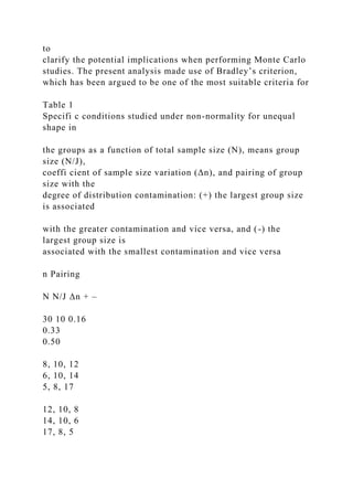
conocidas. Las
variables manipuladas han sido: igualdad o desigualdad del
tamaño de los
grupos, tamaño muestral total y de los grupos; coefi ciente de
variación
del tamaño muestral; forma de la distribución e igualdad o
desigualdad de
la forma en los grupos; y emparejamiento entre el tamaño
muestral con
el grado de contaminación en la distribución. Resultados: los
resultados
muestran que el estadístico F es robusto en términos de error de
Tipo I en
el 100% de los casos estudiados, independientemente de las
condiciones
manipuladas.
Palabras clave: estadístico F, ANOVA, robustez, asimetría,
curtosis.
Psicothema 2017, Vol. 29, No. 4, 552-557
doi: 10.7334/psicothema2016.383
Received: December 14, 2016 • Accepted: June 20, 2017
Corresponding author: María J. Blanca
Facultad de Psicología
Universidad de Málaga
29071 Málaga (Spain)
e-mail: [email protected]
553

and found that, in general, F-test was quite robust, the effect
being
negligible. Likewise, Tiku (1964) stated that distributions with
skewness values in a different direction had a greater effect
than
did those with values in the same direction unless the degrees of
freedom for error were fairly large. However, Glass, Peckham,
and
Sanders (1972) summarized these early studies and concluded
that the procedure was affected by kurtosis, whereas skewness
had very little effect. Conversely, Harwell, Rubinstein, Hayes,
and
Olds (1992), using meta-analytic techniques, found that
skewness
had more effect than kurtosis. A subsequent meta-analytic study
by Lix et al. (1996) concluded that Type I error performance did
not appear to be affected by non-normality.
These inconsistencies may be attributable to the fact that a
standard criterion has not been used to assess robustness, thus
leading to different interpretations of the Type I error rate. The
use
of a single and standard criterion such as that proposed by
Bradley
(1978) would be helpful in this context. According to Bradley’s
(1978) liberal criterion a statistical test is considered robust if
the
empirical Type I error rate is between .025 and .075 for a
nominal
alpha level of .05. In fact, had Bradley’s criterion of robustness
been adopted in the abovementioned studies, many of their
results
would have been interpreted differently, leading to different
conclusions. Furthermore, when this criterion is considered,
more

recent studies provide empirical evidence for the robustness of
F-test under non-normality with homogeneity of variances
(Black
et al., 2010; Clinch & Keselman, 1982; Feir-Walsh &
Thoothaker,
1974; Gamage & Weerahandi, 1998; Kanji, 1976; Lantz, 2013;
Patrick, 2007; Schmider et al., 2010; Zijlstra, 2004).
Based on most early studies, many classical handbooks on
research methods in education and psychology draw the
following
conclusions: Moderate departures from normality are of little
concern in the fi xed-effects analysis of variance (Montgomery,
1991); violations of normality do not constitute a serious
problem,
unless the violations are especially severe (Keppel, 1982); F-
test is
robust to moderate departures from normality when sample sizes
are
reasonably large and are equal (Winer, Brown, & Michels,
1991); and
researchers do not need to be concerned about moderate
departures
from normality provided that the populations are homogeneous
in
form (Kirk, 2013). To summarize, F-test is robust to departures
from
normality when: a) the departure is moderate; b) the populations
have the same distributional shape; and c) the sample sizes are
large
and equal. However, these conclusions are broad and
ambiguous,
and they are not helpful when it comes to deciding whether or
not
F-test can be used. The main problem is that expressions such
as

“moderate”, “severe” and “reasonably large sample size” are
subject
to different interpretations and, consequently, they do not
constitute
a standard guideline that helps applied researchers decide
whether
they can trust their F-test results under non-normality.
Given this situation, the main goals of the present study are to
provide a systematic examination of F-test robustness, in terms
of Type I error, to violations of normality under homogeneity
using a standard criterion such as that proposed by Bradley
(1978). Specifi cally, we aim to answer the following questions:
Is
F-test robust to slight and moderate departures from normality?
Is it robust to severe departures from normality? Is it sensitive
to differences in shape among the groups? Does its robustness
depend on the sample sizes? Is its robustness associated with
equal
or unequal sample sizes?
To this end, we designed a Monte Carlo simulation study to
examine the effect of a wide variety of distributions commonly
found in the health and social sciences on the robustness of F-
test.
Distributions with a slight and moderate degree of
contamination
(Blanca et al., 2013) were simulated by generating distributions
with values of skewness and kurtosis ranging between -1 and 1.
Distributions with a severe degree of contamination (Micceri,
1989) were represented by exponential, double exponential, and
chi-square with 8 degrees of freedom. In both cases, a wide
range
of sample sizes were considered with balanced and unbalanced
designs and with equal and unequal distributions in groups.

With
unequal sample size and unequal shape in the groups, the
pairing
of group sample size with the degree of contamination in the
distribution was also investigated.
Method
Instruments
We conducted a Monte Carlo simulation study with non-
normal data using SAS 9.4. (SAS Institute, 2013). Non-normal
distributions were generated using the procedure proposed by
Fleishman (1978), which uses a polynomial transformation to
generate data with specifi c values of skewness and kurtosis.
Procedure
In order to examine the effect of non-normality on F-test
robustness, a one-way design with 3 groups and homogeneity of
variance was considered. The group effect was set to zero in the
population model. The following variables were manipulated:
1. Equal and unequal group sample sizes. Unbalanced designs
are more common than balanced designs in studies involving
one-way and factorial ANOVA (Golinski & Cribbie, 2009;
Keselman et al., 1998). Both were considered in order to
extend our results to different research situations.
2. Group sample size and total sample size. A wide range of
group sample sizes were considered, enabling us to study
small, medium, and large sample sizes. With balanced
designs the group sizes were set to 5, 10, 15, 20, 25, 30, 40,
50, 60, 70, 80, 90, and 100, with total sample size ranging
from 15 to 300. With unbalanced designs, group sizes were
set between 5 and 160, with a mean group size of between

10 and 100 and total sample size ranging from 15 to 300.
3. Coeffi cient of sample size variation (Δn), which represents
the amount of inequality in group sizes. This was computed
by dividing the standard deviation of the group sample size
by its mean. Different degrees of variation were considered
and were grouped as low, medium, and high. A low Δn
was fi xed at approximately 0.16 (0.141 - 0.178), a medium
coeffi cient at 0.33 (0.316 - 0.334), and a high value at 0.50
(0.491 - 0.521). Keselman et al. (1998) showed that the ratio
of the largest to the smallest group size was greater than 3
in 43.5% of cases. With Δn = 0.16 this ratio was equal to 1.5,
with Δn = 0.33 it was equal to either 2.3 or 2.5, and with Δn
= 0.50 it ranged from 3.3 to 5.7.
4. Shape of the distribution and equal and unequal shape in
the groups. Twenty-two distributions were investigated,
involving several degrees of deviation from normality and
with both equal and unequal shape in the groups. For equal
shape and slight and moderate departures from normality,
Rebecca Bendayan
554
the distributions had values of skewness (γ
1
) and kurtosis (γ
2
)
ranging between -1 and 1, these values being representative

of real data (Blanca et al., 2013). The values of γ
1
and γ
2
are presented in Table 2 (distributions 1-12). For severe
departures from normality, distributions had values of γ
1
and
γ
2
corresponding to the double exponential, chi-square with
8 degrees of freedom, and exponential distributions (Table
2, distributions 13-15). For unequal shape, the values of γ
1
and γ
2
of each group are presented in Table 3. Distributions
16-21 correspond to slight and moderate departures from
normality and distribution 22 to severe departure.
5. Pairing of group size with degree of contamination in the
distribution. This condition was included with unequal
shape and unequal sample size. The pairing was positive
when the largest group size was associated with the greater
contamination, and vice versa. The pairing was negative
when the largest group size was associated with the smallest

contamination, and vice versa. The specifi c conditions with
unequal sample size are shown in Table 1.
Ten thousand replications of the 1308 conditions resulting
from the combination of the above variables were performed at
a
signifi cance level of .05. This number of replications was
chosen
to ensure reliable results (Bendayan, Arnau, Blanca, & Bono,
2014; Robey & Barcikowski, 1992).
Data analysis
Empirical Type I error rates associated with F-test were
analyzed for each condition according to Bradley’s robustness
criterion (1978).
Results
Tables 2 and 3 show descriptive statistics for the Type I error
rate across conditions for equal and unequal shapes. Although
the
tables do not include all available information (due to article
length
limitations), the maximum and minimum values are suffi cient
for
assessing robustness. Full tables are available upon request
from
the corresponding author.
All empirical Type I error rates were within the bounds of
Bradley’s criterion. The results show that F-test is robust for 3
groups in 100% of cases, regardless of the degree of deviation
from a normal distribution, sample size, balanced or unbalanced
cells, and equal or unequal distribution in the groups.

Discussion
We aimed to provide a systematic examination of F-test
robustness to violations of normality under homogeneity of
variance, applying Bradley’s (1978) criterion. Specifi cally, we
sought to answer the following question: Is F-test robust, in
terms
of Type I error, to slight, moderate, and severe departures from
normality, with various sample sizes (equal or unequal sample
size) and with same or different shapes in the groups? The
answer
to this question is a resounding yes, since F-test controlled
Type
I error to within the bounds of Bradley’s criterion. Specifi cally,
the results show that F-test remains robust with 3 groups when
distributions have values of skewness and kurtosis ranging
between -1 and 1, as well as with data showing a greater
departure
from normality, such as the exponential, double exponential,
and
chi-squared (8) distributions. This applies even when sample
sizes
are very small (i.e., n= 5) and quite different in the groups, and
also when the group distributions differ signifi cantly. In
addition,
the test’s robustness is independent of the pairing of group size
with the degree of contamination in the distribution.
Our results support the idea that the discrepancies between
studies on the effect of non-normality may be primarily
attributed
to differences in the robustness criterion adopted, rather than to
the degree of contamination of the distributions. These fi ndings
highlight the need to establish a standard criterion of robustness

to
clarify the potential implications when performing Monte Carlo
studies. The present analysis made use of Bradley’s criterion,
which has been argued to be one of the most suitable criteria for
Table 1
Specifi c conditions studied under non-normality for unequal
shape in
the groups as a function of total sample size (N), means group
size (N/J),
coeffi cient of sample size variation (Δn), and pairing of group
size with the
degree of distribution contamination: (+) the largest group size
is associated
with the greater contamination and vice versa, and (-) the
largest group size is
associated with the smallest contamination and vice versa
n Pairing
N N/J Δn + –
30 10 0.16
0.33
0.50
8, 10, 12
6, 10, 14
5, 8, 17
12, 10, 8
14, 10, 6
17, 8, 5

45 15 0.16
0.33
0.50
12, 15, 18
9, 15, 21
6, 15, 24
18, 15, 12
21, 15, 9
24, 15, 6
60 20 0.16
0.33
0.50
16, 20, 24
12, 20, 28
8, 20, 32
24, 20, 16
28, 20, 12
32, 20, 8
75 25 0.16
0.33
0.50
20, 25, 30
15, 25, 35
10, 25, 40
30, 25, 20
35, 25, 15
40, 25, 10

90 30 0.16
0.33
0.50
24, 30, 36
18, 30, 42
12, 30, 48
36, 30, 24
42, 30, 18
48, 30, 12
120 40 0.16
0.33
0.50
32, 40, 48
24, 40, 56
16, 40, 64
48, 40, 32
56, 40, 24
64, 40, 16
150 50 0.16
0.33
0.50
40, 50, 60
30, 50, 70
20, 50, 80
60, 50, 40
70, 50, 30
80, 50, 20

180 60 0.16
0.33
0.50
48, 60, 72
36, 60, 84
24, 60, 96
72, 60, 48
84, 60, 36
96, 60, 24
210 70 0.16
0.33
0.50
56, 70, 84
42, 70, 98
28, 70, 112
84, 70, 56
98, 70, 42
112, 70, 28
240 80 0.16
0.33
0.50
64, 80, 96
48, 80, 112
32, 80, 128
96, 80, 64
112, 80, 48
128, 80, 32

270 90 0.16
0.33
0.50
72, 90, 108
54, 90, 126
36, 90, 144
108, 90, 72
126, 90, 54
144, 90, 36
300 100 0.16
0.33
0.50
80, 100, 120
60, 100, 140
40, 100, 160
120, 100, 80
140, 100, 60
160, 100, 40
555
examining the robustness of statistical tests (Keselman, Algina,
Kowalchuk, & Wolfi nger, 1999). In this respect, our results are
consistent with previous studies whose Type I error rates were
within the bounds of Bradley’s criterion under certain
departures
from normality (Black et al., 2010; Clinch & Keselman, 1982;

Feir-Walsh & Thoothaker, 1974; Gamage & Weerahandi, 1998;
Kanji, 1976; Lantz, 2013; Lix et al., 1996; Patrick, 2007;
Schmider
et al., 2010; Zijlstra, 2004). By contrast, however, our results
do
not concur, at least for the conditions studied here, with those
classical handbooks which conclude that F-test is only robust
if the departure from normality is moderate (Keppel, 1982;
Montgomery, 1991), the populations have the same
distributional
shape (Kirk, 2013), and the sample sizes are large and equal
(Winer et al., 1991).
Our fi ndings are useful for applied research since they show
that, in terms of Type I error, F-test remains a valid statistical
procedure under non-normality in a variety of conditions. Data
transformation or nonparametric analysis is often recommended
when data are not normally distributed. However, data
transformations offer no additional benefi ts over the good
control
of Type I error achieved by F-test. Furthermore, it is usually
diffi cult to determine which transformation is appropriate for a
set
of data, and a given transformation may not be applicable when
groups differ in shape. In addition, results are often diffi cult to
interpret when data transformations are adopted. There are also
disadvantages to using non-parametric procedures such as the
Kruskal-Wallis test. This test converts quantitative continuous
data into rank-ordered data, with a consequent loss of
information.
Moreover, the null hypothesis associated with the Kruskal-
Wallis
test differs from that of F-test, unless the distribution of groups
has exactly the same shape (see Maxwell & Delaney, 2004).
Given

these limitations, there is no reason to prefer the Kruskal-Wallis
test
under the conditions studied in the present paper. Only with
equal
shape in the groups might the Kruskal-Wallis test be preferable,
given its power advantage over F-test under specifi c
distributions
(Büning, 1997; Lantz, 2013). However, other studies suggest
that
F-test is robust, in terms of power, to violations of normality
under
certain conditions (Ferreira, Rocha, & Mequelino, 2012; Kanji,
1976; Schmider et al., 2010), even with very small sample size
(n =
3; Khan & Rayner, 2003). In light of these inconsistencies,
future
research should explore the power of F-test when the normality
assumption is not met. At all events, we encourage researchers
to analyze the distribution underlying their data (e.g., coeffi
cients
of skewness and kurtosis in each group, goodness of fi t tests,
and
normality graphs) and to estimate a priori the sample size
needed
to achieve the desired power.
Table 2
Descriptive statistics of Type I error for F-test with equal shape
for each combination of skewness (γ
1
) and kurtosis (γ
2
) across all conditions

Distributions γ1 γ2 n Min Max Mdn M SD
1 0 0.4 =
≠
.0434
.0445
.0541
.0556
.0491
.0497
.0493
.0496
.0029
.0022
2 0 0.8 =
≠
.0444
.0458
.0534
.0527
.0474
.0484
.0479
.0487

.0023
.0016
3 0 -0.8 =
≠
.0468
.0426
.0512
.0532
.0490
.0486
.0491
.0487
.0014
.0024
4 0.4 0 =
≠
.0360
.0392
.0499
.0534
.0469
.0477
.0457

.0472
.0044
.0032
5 0.8 0 =
≠
.0422
.0433
.0528
.0553
.0477
.0491
.0476
.0491
.0029
.0030
6 -0.8 0 =
≠
.0427
.0457
.0551
.0549
.0475

.0487
.0484
.0492
.0038
.0024
7 0.4 0.4 =
≠
.0426
.0417
.0533
.0533
.0487
.0486
.0488
.0487
.0031
.0026
8 0.4 0.8 =
≠
.0449
.0456
.0516
.0537

.0483
.0489
.0485
.0489
.0019
.0020
9 0.8 0.4 =
≠
.0372
.0413
.0494
.0518
.0475
.0481
.0463
.0475
.0033
.0026
10 0.8 1 =
≠
.0458
.0463
.0517

.0540
.0494
.0502
.0492
.0501
.0017
.0023
11 1 0.8 =
≠
.0398
.0430
.0506
.0542
.0470
.0489
.0463
.0485
.0028
.0029
12 1 1 =
≠
.0377

.0366
.0507
.0512
.0453
.0466
.0451
.0462
.0042
.0032
13 0 3 =
≠
.0443
.0435
.0517
.0543
.0477
.0490
.0479
.0489
.0022
.0024
14 1 3 =
≠

.0431
.0462
.0530
.0548
.0487
.0494
.0486
.0499
.0032
.0017
15 2 6 =
≠
.0474
.0442
.0524
.0526
.0496
.0483
.0497
.0488
.0017
.0022

Rebecca Bendayan
556
As the present study sought to provide a systematic examination
of the independent effect of non-normality on F-test Type I
error
rate, variance homogeneity was assumed. However, previous
studies
have found that F-test is sensitive to violations of homogeneity
assumptions (Alexander & Govern, 1994; Blanca, Alarcón,
Arnau,
& Bono, in press; Büning, 1997; Gamage & Weerahandi, 1998;
Harwell et al., 1992; Lee & Ahn, 2003; Lix et al., 1996; Moder,
2010;
Patrick, 2007; Yiǧit & Gökpinar, 2010; Zijlstra, 2004), and
several
procedures have been proposed for dealing with
heteroscedasticity
(e.g., Alexander & Govern, 1994; Brown-Forsythe, 1974; Chen
&
Chen, 1998; Krishnamoorthy, Lu, & Mathew, 2007; Lee & Ahn,
2003; Li, Wang, & Liang, 2011; Lix & Keselman, 1998;
Weerahandi,
1995; Welch, 1951). This suggests that heterogeneity has a
greater
effect on F-test robustness than does non-normality. Future
research
should therefore also consider violations of homogeneity.
To sum up, the present results provide empirical evidence for
the robustness of F-test under a wide variety of conditions
(1308)

involving non-normal distributions likely to represent real data.
Researchers can use these fi ndings to determine whether F-test
is
a valid option when testing hypotheses about means in their
data.
Acknowledgements
This research was supported by grants PSI2012-32662 and
PSI2016-78737-P (AEI/FEDER, UE; Spanish Ministry of
Economy, Industry, and Competitiveness).
Table 3
Descriptive statistics of Type I error for F-test with unequal
shape for each combination of skewness (γ
1
) and kurtosis (γ
2
) across all conditions
Distributions Group γ1 γ2 n Min Max Mnd M SD
16 1
2
3
0
0
0
0.2
0.4
0.6

=
≠
.0434
.0433
.0541
.0540
.0491
.0490
.0493
.0487
.0029
.0025
17 1
2
3
0
0
0
0.2
0.4
-0.6
=
≠
.0472

.0409
.0543
.0579
.0513
.0509
.0509
.0510
.0024
.0033
18 1
2
3
0.2
0.4
0.6
0
0
0
=
≠
.0426
.0409
.0685
.0736
.0577

.0563
.0578
.0569
.0077
.0072
19 1
2
3
0.2
0.4
-0.6
0
0
0
=
≠
.0481
.0449
.0546
.0574
.0501
.0497
.0504
.0499

.0020
.0024
20 1
2
3
0.2
0.4
0.6
0.4
0.6
0.8
=
≠
.0474
.0433
.0524
.0662
.0496
.0535
.0497
.0545
.0017
.0057
21 1

2
3
0.2
0.6
1
0.4
0.8
1.2
=
≠
.0462
.0419
.0537
.0598
.0503
.0499
.0501
.0502
.0024
.0025
22 1
2
3
0
1

2
3
3
6
=
≠
.0460
.0424
.0542
.0577
.0490
.0503
.0494
.0499
.0027
.0029
References
Alexander, R. A., & Govern, D. M. (1994). A new and simpler
approximation for ANOVA under variance heterogeneity.
Journal of
Educational and Behavioral Statistics, 19, 91-101.
Bendayan, R., Arnau, J., Blanca, M. J., & Bono, R. (2014).
Comparison of
the procedures of Fleishman and Ramberg et al., for generating
non-

normal data in simulation studies. Anales de Psicología, 30,
364-371.
Black, G., Ard, D., Smith, J., & Schibik, T. (2010). The impact
of the
Weibull distribution on the performance of the single-factor
ANOVA
model. International Journal of Industrial Engineering
Computations,
1, 185-198.
Blanca, M. J., Alarcón, R., Arnau, J., & Bono, R. (in press).
Effect of
variance ratio on ANOVA robustness: Might 1.5 be the limit?
Behavior
Research Methods.
Blanca, M. J., Arnau, J., López-Montiel, D., Bono, R., &
Bendayan, R. (2013).
Skewness and kurtosis in real data samples. Methodology, 9,
78-84.
Bradley, J. V. (1978). Robustness? British Journal of
Mathematical and
Statistical Psychology, 31, 144-152.
Brown, M.B., & Forsythe, A.B. (1974). The small sample
behaviour of some
statistics which test the equality of several means.
Technomectrics, 16,
129-132.
Büning, H. (1997). Robust analysis of variance. Journal of
Applied
Statistics, 24, 319-332.

Chen, S.Y., & Chen, H.J. (1998). Single-stage analysis of
variance under
heteroscedasticity. Communications in Statistics – Simulation
and
Computation, 27, 641-666.
Clinch, J. J., & Kesselman, H. J. (1982). Parametric alternatives
to the
analysis of variance. Journal of Educational Statistics, 7, 207-
214.
Feir-Walsh, B. J., & Thoothaker, L. E. (1974). An empirical
comparison
of the ANOVA F-test, normal scores test and Kruskal-Wallis
test
under violation of assumptions. Educational and Psychological
Measurement, 34, 789-799.
Ferreira, E. B., Rocha, M. C., & Mequelino, D. B. (2012).
Monte Carlo
evaluation of the ANOVA’s F and Kruskal-Wallis tests under
binomial
distribution. Sigmae, 1, 126-139.
557
Fleishman, A. I. (1978). A method for simulating non-normal
distributions.
Psychometrika, 43, 521-532.
Gamage, J., & Weerahandi, S. (1998). Size performance of some
tests in

one-way ANOVA. Communications in Statistics - Simulation
and
Computation, 27, 625-640.
Glass, G. V., Peckham, P. D., & Sanders, J. R. (1972).
Consequences of failure
to meet assumptions underlying the fi xed effects analyses of
variance
and covariance. Review of Educational Research, 42, 237-288.
Golinski, C., & Cribbie, R. A. (2009). The expanding role of
quantitative
methodologists in advancing psychology. Canadian Psychology,
50,
83-90.
Harvey, C., & Siddique, A. (2000). Conditional skewness in
asset pricing
test. Journal of Finance, 55, 1263-1295.
Harwell, M. R., Rubinstein, E. N., Hayes, W. S., & Olds, C. C.
(1992).
Summarizing Monte Carlo results in methodological research:
The one- and two-factor fi xed effects ANOVA cases. Journal of
Educational and Behavioral Statistics, 17, 315-339.
Kanji, G. K. (1976). Effect of non-normality on the power in
analysis of
variance: A simulation study. International Journal of
Mathematical
Education in Science and Technology, 7, 155-160.
Keppel, G. (1982). Design and analysis. A researcher’s
handbook (2nd
ed.). New Jersey: Prentice-Hall.

Keselman, H. J., Algina, J., Kowalchuk, R. K., & Wolfi nger, R.
D. (1999).
A comparison of recent approaches to the analysis of repeated
measurements. British Journal of Mathematical and Statistical
Psychology, 52, 63-78.
Keselman, H. J., Huberty, C. J., Lix, L. M., Olejnik, S., Cribbie,
R. A.,
Donahue, B.,..., Levin, J. R. (1998). Statistical practices of
educational
researchers: An analysis of their ANOVA, MANOVA, and
ANCOVA
analyses. Review of Educational Research, 68, 350-386.
Khan, A., & Rayner, G. D. (2003). Robustness to non-normality
of
common tests for the many-sample location problem. Journal of
Applied Mathematics and Decision Sciences, 7, 187-206.
Kieffer, K. M., Reese, R. J., & Thompson, B. (2001). Statistical
techniques
employed in AERJ and JCP articles from 1988 to 1997: A
methodological
review. The Journal of Experimental Education, 69, 280-309.
Kirk, R. E. (2013). Experimental design. Procedures for the
behavioral
sciences (4th ed.). Thousand Oaks: Sage Publications.
Kobayashi, K. (2005). Analysis of quantitative data obtained
from toxicity
studies showing non-normal distribution. The Journal of
Toxicological
Science, 30, 127-134.
Krishnamoorthy, K., Lu, F., & Mathew, T. (2007). A parametric

bootstrap
approach for ANOVA with unequal variances: Fixed and
random
models. Computational Statistics & Data Analysis 51, 5731-
5742.
Lantz, B. (2013). The impact of sample non-normality on
ANOVA and
alternative methods. British Journal of Mathematical and
Statistical
Psychology, 66, 224-244.
Lee, S., & Ahn, C. H. (2003). Modifi ed ANOVA for unequal
variances.
Communications in Statistics - Simulation and Computation, 32,
987-
1004.
Li, X., Wang, J., & Liang, H. (2011). Comparison of several
means: A
fi ducial based approach. Computational Statistics and Data
Analysis,
55, 1993-2002.
Lindquist, E. F. (1953). Design and analysis of experiments in
psychology
and education. Boston: Houghton Miffl in.
Lix, L.M., & Keselman, H.J. (1998). To trim or not to trim:
Tests of mean
equality under heteroscedasticity and nonnormality. Educational
and
Psychological Measurement, 58, 409-429.
Lix, L. M., Keselman, J. C., & Keselman, H. J. (1996).
Consequences of

assumption violations revisited: A quantitative review of
alternatives
to the one-way analysis of variance F test. Review of
Educational
Research, 66, 579-619.
Maxwell, S. E., & Delaney, H. D. (2004). Designing
experiments and
analyzing data: A model comparison perspective (2nd ed.).
Mahwah:
Lawrence Erlbaum Associates.
Micceri, T. (1989). The unicorn, the normal curve, and other
improbable
creatures. Psychological Bulletin, 105, 156-166.
Moder, K. (2010). Alternatives to F-test in one way ANOVA in
case of
heterogeneity of variances (a simulation study). Psychological
Test
and Assessment Modeling, 52, 343-353.
Montgomery, D. C. (1991). Design and analysis of experiments
(3rd ed.).
New York, NY: John Wiley & Sons, Inc.
Patrick, J. D. (2007). Simulations to analyze Type I error and
power in
the ANOVA F test and nonparametric alternatives (Master’s
thesis,
University of West Florida). Retrieved from
http://etd.fcla.edu/WF/
WFE0000158/Patrick_Joshua_Daniel_200905_MS.pdf
Pearson, E. S. (1931). The analysis of variance in cases of non-
normal

variation. Biometrika, 23, 114-133.
Robey, R. R., & Barcikowski, R. S. (1992). Type I error and the
number
of iterations in Monte Carlo studies of robustness. British
Journal of
Mathematical and Statistical Psychology, 45, 283-288.
SAS Institute Inc. (2013). SAS® 9.4 guide to software Updates.
Cary:
SAS Institute Inc.
Schmider, E., Ziegler, M., Danay, E., Beyer, L., & Bühner, M.
(2010). Is
it really robust? Reinvestigating the robustness of ANOVA
against
violations of the normal distribution assumption. Methodology,
6, 147-
151.
Tiku, M. L. (1964). Approximating the general non-normal
variance-ratio
sampling distributions. Biometrika, 51, 83-95.
Van Der Linder, W. J. (2006). A lognormal model for response
times on
test items. Journal of Educational and Behavioral Statistics, 31,
181-
204.
Welch, B.L. (1951). On the comparison of several mean values:
An
alternative approach. Biometrika, 38, 330-336.
Weerahandi, S. (1995). ANOVA under unequal error variances.
Biometrics,

51, 589-599.
Winer, B. J., Brown, D. R., & Michels, K. M. (1991). Statistical
principles
in experimental design (3rd ed.). New York: McGraw-Hill.
Yiğit, E., & Gökpınar, F. (2010). A Simulation study on tests
for one-way
ANOVA under the unequal variance assumption.
Communications
Faculty of Sciences University of Ankara, Series A1, 59, 15-34.
Zijlstra, W. (2004). Comparing the Student´s t and the ANOVA
contrast
procedure with fi ve alternative procedures (Master’s thesis,
Rijksuniversiteit Groningen). Retrieved from
http://www.ppsw.rug.
nl/~kiers/ReportZijlstra.pdf
Copyright of Psicothema is the property of Colegio Oficial de
Psicologos del Principado de
Asturias and its content may not be copied or emailed to
multiple sites or posted to a listserv
without the copyright holder's express written permission.
However, users may print,
download, or email articles for individual use.

ANOVA Interpretation Set 1 Study this scenario and ANOVA.docx

More Related Content

Similar to ANOVA Interpretation Set 1 Study this scenario and ANOVA.docx

More from festockton

Recently uploaded

ANOVA Interpretation Set 1 Study this scenario and ANOVA.docx