1. Point-to-Point Shortest Path Algorithms
with Preprocessing
Andrew V. Goldberg
Microsoft Research – Silicon Valley
www.research.microsoft.com/∼goldberg/
Joint with Haim Kaplan and Renato Werneck

2. Einstein Quote
Everything should be made as simple as possible, but not simpler
SP with preprocessing 1

3. Shortest Path Problem
Variants
• Nonnegative and arbitrary arc lengths.
• Point to point, single source, all pairs.
• Directed and undirected.
Here we study
• Point to point, nonnegative length, directed problem.
• Allow preprocessing with limited (linear) space.
Many applications, both directly and as a subroutine.
SP with preprocessing 2

4. Shortest Path Problem
Input: Directed graph G = (V, A), nonnegative length function
: A → R+ , origin s ∈ V , destination t ∈ V .
Preprocessing: Limited space to store results.
Query: Find a shortest path from s to t.
Interested in exact algorithms that search a (small) subgraph.
Related work: reach-based routing [Gutman 04], hierarchi-
cal decomposition [Schultz, Wagner & Weihe 02], [Sanders &
Schultes 05, 06], geometric pruning [Wagner & Willhalm 03], arc
flags [Lauther 04], [K¨hler, M¨hring & Schilling 05], [M¨hring
o o o
et al. 06].
SP with preprocessing 3

5. Motivating Application
Driving directions
• Run on servers and small devices.
• Typical production codes
◦ Use base graph or other heuristics based on road cate-
gories; needs hand-tuning.
◦ Runs (bidirectional) Dijkstra or A∗ with Euclidean bounds
on “patched” graph.
◦ Non-exact and no performance guarantee.
• We are interested in exact and very efficient algorithms.
• New results finding their way into products.
SP with preprocessing 4

6. Outline
• Scanning method and Dijkstra’s algorithm.
• Bidirectional Dijkstra’s algorithm.
• A∗ search.
• ALT Algorithm
• Definition of reach
• Reach-based algorithm
• Reach for A∗
SP with preprocessing 5

7. Scanning Method
• For each vertex v maintain its distance label ds(v) and status
S(v) ∈ {unreached, labeled, scanned}.
• Unreached vertices have ds(v) = ∞.
• If ds(v) decreases, v becomes labeled.
• To scan a labeled vertex v, for each arc (v, w),
if ds(w) > ds(v) + (v, w) set ds (w) = ds(v) + (v, w).
• Initially for all vertices are unreached.
• Start by decreasing ds(s) to 0.
• While there are labeled vertices, pick one and scan it.
• Different selection rules lead to different algorithms.
SP with preprocessing 6

8. Dijkstra’s Algorithm
[Dijkstra 1959], [Dantzig 1963].
• At each step scan a labeled vertex with the minimum label.
• Stop when t is selected for scanning.
Work almost linear in the visited subgraph size.
Reverse Algorithm: Run algorithm from t in the graph with all
arcs reversed, stop when t is selected for scanning.
Bidirectional Algorithm
• Run forward Dijkstra from s and backward from t.
• Maintain µ, the length of the shortest path seen: when scan-
ning an arc (v, w) such that w has been scanned in the other
direction, check if the corresponding s-t path improves µ.
• Stop when about to scan a vertex x scanned in the other
direction.
• Output µ and the corresponding path.
SP with preprocessing 7

9. Bidirectional Algorithm: Pitfalls
The algorithm is not as simple as it looks.
2 a 5 b 2
s t
5 x 5
The searches meat at x, but x is not on the shortest path.
SP with preprocessing 8

10. Example Graph
1.6M vertices, 3.8M arcs, travel time metric.
SP with preprocessing 9

11. Dijkstra’s Algorithm
Searched area
SP with preprocessing 10

12. Bidirectional Algorithm
forward search/ reverse search
SP with preprocessing 11

13. A∗ Search
[Doran 67], [Hart, Nilsson & Raphael 68]
Motivated by large search spaces (e.g., game graphs).
Similar to Dijkstra’s algorithm but:
• Domain-specific estimates πt(v) on dist(v, t) (potentials).
• At each step pick a labeled vertex with the minimum k(v) =
ds(v) + πt(v).
Best estimate of path length.
• In general, optimality is not guaranteed.
1
11
00
111111
000000
2
1
0
1111111
3
11
00
111111
0
4
1
0
00000000000000000
111111
0 1111111
0000000
11
00
111111
000000 1
0 11
00 1
0
1111111
0000000
11
00
111111
000000 1
0 11
00 1
0
1111111
0000000
111111
000000
0 4
111111
000000 3 2 1111111
0000000
1 5
1111111
0000000
11111111111
00000000000
111111
000000
1
0
11111111111
00000000000 1111111
0000000
1
0
1111111
0000000
1
0
11111111111
00000000000 1
0
1111111
0000000
11111111111
00000000000 1111111
0000000
0
11111111111
00000000000
11111111111
00000000000 1111111
0000000
1111111
0000000
1
0
1
0 11
00
111111 1
0
00000000000
111111
0
11
00 1
0
6 2 1
SP with preprocessing 12

14. Feasibility and Optimality
Potential transformation: Replace (v, w) by
πt (v, w) = (v, w) − πt(v) + πt(w) (reduced costs).
Fact: Problems defined by and πt are equivalent.
Definition: πt is feasible if ∀(v, w) ∈ A, the reduced costs are
nonnegative. (Estimates are “locally consistent”.)
Optimality: If πt is feasible, the A∗ search is equivalent to Dijk-
stra’s algorithm on transformed network, which has nonnegative
arc lengths. A∗ search finds an optimal path.
Different order of vertex scans, different subgraph searched.
Fact: If πt is feasible and πt(t) = 0, then πt gives lower bounds
on distances to t.
SP with preprocessing 13

15. Computing Lower Bounds
Euclidean bounds:
[folklore], [Pohl 71], [Sedgewick & Vitter 86].
For graph embedded in a metric space, use Euclidean distance.
Limited applicability, not very good for driving directions.
We use triangle inequality
a000
1111111111111
0000000000000
111
b
11111111111111
00000000000000
111
000
11 11111111111111
00 00000000000000
1111111111111
0000000000000
111
000 1
0
111
000
11 11111111111111
00 00000000000000
1111111111111
0000000000000
111
000 1
0
111
000
1111111111111
0000000000000
111
000
11111111111111
00000000000000
1111111111111
0000000000000
111
000 111
000
11111111111111
00000000000000
111
000
1
0 11
00
1111111111111
0000000000000
111
000
11111111111111
00000000000000
11111111111111
00000000000000
1
0
1
0
11
00
11
00
v w
dist(v, w) ≥ dist(v, b)−dist(w, b); dist(v, w) ≥ dist(a, w)−dist(a, v).
SP with preprocessing 14

16. Lower Bounds (cont.)
Maximum (minimum, average) of feasible potentials is feasible.
• Select landmarks (a small number).
• For all vertices, precompute distances to and from each land-
mark.
• For each s, t, use max of the corresponding lower bounds for
πt(v).
Why this works well (when it does)
a
s x y t
πt (x, y) = 0
SP with preprocessing 15

17. Bidirectional Lowerbounding
Forward reduced costs: πt (v, w) = (v, w) − πt(v) + πt(w).
Reverse reduced costs: πs (v, w) = (v, w) + πs(v) − πs(w).
What’s the problem?
SP with preprocessing 16

18. Bidirectional Lowerbounding
Forward reduced costs: πt (v, w) = (v, w) − πt(v) + πt(w).
Reverse reduced costs: πs (v, w) = (v, w) + πs(v) − πs(w).
Fact: πt and πs give the same reduced costs iff πs + πt = const.
[Ikeda et at. 94]: use ps(v) = πs(v)−πt(v) and pt (v) = −ps(v).
2
Other solutions possible. Easy to loose correctness.
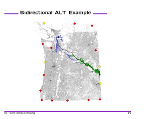
ALT algorithms use A∗ search and landmark-based lower bounds.
SP with preprocessing 17

19. Landmark Selection
Preprocessing
• Random selection is fast.
• Many heuristics find better landmarks.
• Local search can find a good subset of candidate landmarks.
• We use a heuristic with local search.
Preprocessing/query trade-off.
Query
• For a specific s, t pair, only some landmarks are useful.
• Use only active landmarks that give best bounds on dist(s, t).
• If needed, dynamically add active landmarks (good for the
search frontier).
Allows using many landmarks with small time overhead.
SP with preprocessing 18

20. Bidirectional ALT Example
SP with preprocessing 19

21. Experimental Results
Northwest (1.6M vertices), random queries, 16 landmarks.
preprocessing query
method minutes MB avgscan maxscan ms
Bidirectional Dijkstra — 28 518 723 1 197 607 340.74
ALT 4 132 16 276 150 389 12.05
SP with preprocessing 20

22. Related Systems Work
Network delay estimation:
Use delays to beacons to estimate arbitrary node delays.
E.g., IDMaps [Francis et al. 01].
Theoretical analysis [Kleinberg, Slivkins & Wexler 04]: for ran-
dom beacons and bounded doubling dimension graphs, get good
bounds for most node pairs.
Good bounds are not enough to prove bounds on ALT.
SP with preprocessing 21

23. Reach Intuition
Identify local intersections and prune them when searching far
from s and t.
SP with preprocessing 22

24. Reaches
[Gutman 04]
• Consider a vertex v that splits a path P into P1 and P2.
rP (v) = min( (P1), (P2)).
• r(v) = maxP (rP (v)) over all shortest paths P through v.
Using reaches to prune Dijkstra:
LB(w,t)
d(s,v) v w
s t
If r(w) < min(d(v) + (v, w), LB(w, t)) then prune w.
SP with preprocessing 23

25. Obtaining Lower Bounds
Can use landmark lower bounds if available.
Bidirectional search gives implicit bounds (Rt below).
LB(w,t)
d(s,v) v w
s Rt t
Reach-based query algorithm is Dijkstra’s algorithm with prun-
ing based on reaches. Given a lower-bound subroutine, a small
change to Dijkstra’s algorithm.
SP with preprocessing 24

26. Computing Reaches
• A natural exact computation uses all-pairs shortest paths.
• Overnight for 0.3M vertex graph, years for 30M vertex graph.
• Have a heuristic improvement, but it is not fast enough.
• Can use reach upper bounds for query search pruning.
Iterative approximation algorithm: [Gutman 04]
• Use partial shortest path trees of depth O( ) to bound reaches
of vertices v with r(v) < .
• Delete vertices with bounded reaches, add penalties.
• Increase and repeat.
Query time does not increase much; preprocessing faster but still
not fast enough.
SP with preprocessing 25

27. Reach Algorithm
SP with preprocessing 26

28. Experimental Results
Northwest (1.6M vertices), random queries, 16 landmarks.
preprocessing query
method minutes MB avgscan maxscan ms
Bidirectional Dijkstra — 28 518 723 1 197 607 340.74
ALT 4 132 16 276 150 389 12.05
Reach 1 100 34 53 888 106 288 30.61
SP with preprocessing 27

29. Shortcuts
• Consider the graph below.
• Many vertices have large reach.
1000 1000
10 10 10 10 10 10 10 10
s 1000 1010 1020 1030 1040 1030 1020 1010 1000 t
SP with preprocessing 28

30. Shortcuts
• Consider the graph below.
• Many vertices have large reach.
• Add a shortcut arc, break ties by the number of hops.
80
1000 1000
10 10 10 10 10 10 10 10
s t
SP with preprocessing 29

31. Shortcuts
• Consider the graph below.
• Many vertices have large reach.
• Add a shortcut arc, break ties by the number of hops.
• Reaches decrease.
s 1000 60 50 40 30 40 50 60 1000 t
SP with preprocessing 30

32. Shortcuts
• Consider the graph below.
• Many vertices have large reach.
• Add a shortcut arc, break ties by the number of hops.
• Reaches decrease.
• Repeat.
s 1000 20 10 20 30 20 10 20 1000 t
SP with preprocessing 31

33. Shortcuts
• Consider the graph below.
• Many vertices have large reach.
• Add a shortcut arc, break ties by the number of hops.
• Reaches decrease.
• Repeat.
• A small number of shortcuts can greatly decrease many reaches.
s 1000 0 10 0 30 0 10 0 1000 t
SP with preprocessing 32

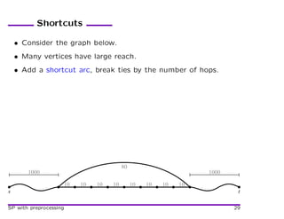
34. Shortcuts
[Sanders & Schultes 05, 06]: similar idea in hierarchy-based al-
gorithm; similar performance.
• During preprocessing we shortcut small-degree vertices every
time is updated.
• Shortcut replaces a vertex by a clique on its neighbors.
• A constant number of arcs is added for each deleted vertex.
• Shortcuts greatly speed up preprocessing.
• Shortcuts speed up queries.
SP with preprocessing 33

35. Reach with Shortcuts
SP with preprocessing 34

36. Experimental Results
Northwest (1.6M vertices), random queries, 16 landmarks.
preprocessing query
method minutes MB avgscan maxscan ms
Bidirectional Dijkstra — 28 518 723 1 197 607 340.74
ALT 4 132 16 276 150 389 12.05
Reach 1 100 34 53 888 106 288 30.61
Reach+Short 17 100 2 804 5 877 2.39
SP with preprocessing 35

37. Reaches and ALT
• ALT computes transformed and original distances.
• ALT can be combined with reach pruning.
• Careful: Implicit lower bounds do not work, but landmark
lower bounds do.
• Shortcuts do not affect landmark distances and bounds.
SP with preprocessing 36

38. Reach with Shortcuts and ALT
SP with preprocessing 37

39. Experimental Results
Northwest (1.6M vertices), random queries, 16 landmarks.
preprocessing query
method minutes MB avgscan maxscan ms
Bidirectional Dijkstra — 28 518 723 1 197 607 340.74
ALT 4 132 16 276 150 389 12.05
Reach 1 100 34 53 888 106 288 30.61
Reach+Short 17 100 2 804 5 877 2.39
Reach+Short+ALT 21 204 367 1 513 0.73
SP with preprocessing 38

40. Further Improvements
• Improved locality (sort by reach).
• For RE, factor of 3 − 12 improvement for preprocessing and
factor of 2 − 4 for query times.
• Reach-aware landmarks: time/space trade-off.
• Idea: maintain landmark distances for a small fraction of
high-reach vertices only.
• Can use more landmarks and improve both time and space.
Practical even for large (USA, Europe) graphs
• ≈ 1 ms. query time on a server.
• ≈ 5sec. query time on a Pocket PC with 2GB flash card.
• Better for local queries.
SP with preprocessing 39

41. The USA Graph
USA: 24M vertices, 58M arcs, time metric, random queries.
preprocessing query
method min KB avgscan maxscan ms
Dijkstra — 536 11 808 864 — 5 440.49
ALT(16) 17.6 2 563 187 968 2 183 718 295.44
Reach impractical
Reach+Short 27.9 893 2 405 4 813 1.77
Reach+Short+ALT(16,1) 45.5 3 032 592 2 668 0.80
Reach+Short+ALT(64,16) 113.9 1 579 538 2 534 0.86
SP with preprocessing 40

42. The USA Graph
USA: 24M vertices, 58M arcs, distance metric, random queries.
preprocessing query
method min KB avgscan maxscan ms
Dijkstra — 536 11 782 104 — 4 576.02
ALT(16) 15.2 2 417 276 195 2 910 133 410.73
Reach impractical
Reach+Short 46.4 918 7 311 13 886 5.78
Reach+Short+ALT(16,1) 61.5 2 923 905 5 510 1.41
Reach+Short+ALT(64,16) 120.5 1 575 670 3 499 1.22
SP with preprocessing 41

43. Europe Graph
Europe: 18M vertices, 43M arcs, time metric, random queries.
preprocessing query
method min KB avgscan maxscan ms
Dijkstra — 393 8 984 289 — 4 365.81
ALT(16) 12.5 1 597 82 348 993 015 120.09
Reach impractical
Reach+Short 45.1 648 4 371 8 486 3.06
Reach+Short+ALT(16,1) 57.7 1 869 714 3 387 0.89
Reach+Short+ALT(64,16) 102.6 1 037 610 2 998 0.91
SP with preprocessing 42

44. Grid Graphs
Grid with uniform random lengths (0.5M vertices), 16 landmarks.
No highway structure.
preprocessing query
method min MB avgscan maxscan ms
Bidirectional Dijkstra — 18.0 174 150 416 925 160.14
ALT 0.26 96.6 6 057 65 664 6.28
Reach+Short 7.77 27.7 6 458 10 049 4.75
Reach+Short+ALT(16,1) 8.03 106.3 558 3 189 0.89
Reach+Short+ALT(64,16) 9.14 49.2 2 823 3 711 2.67
Reach preprocessing expensive, but helps queries.
(64,16) significantly slower that (16,1).
SP with preprocessing 43

45. Demo
SP with preprocessing 44

46. Concluding Remarks
• Our heuristics work well on road networks.
• Recent improvements: [Bast et al. 07, Geisberger et al. 08].
• How to select good shortcuts? (Road networks/grids.)
• For which classes of graphs do these techniques work?
• Need theoretical analysis for interesting graph classes.
• Interesting problems related to reach, e.g.
◦ Is exact reach as hard as all-pairs shortest paths?
˜
◦ Constant-ratio upper bounds on reaches in O(m) time.
• Dynamic graphs (real-time traffic).
SP with preprocessing 45