This document discusses the development of an efficient intrusion detection system (IDS) that employs a custom feature set derived from the UNSW-NB15 dataset to improve prediction accuracy and reduce false-negative rates in identifying network attacks. The proposed model utilizes meta-heuristic optimization techniques such as Flower Pollination Algorithm (FPA) and Minimal Redundancy Maximizing Relevance (mRMR) to enhance feature selection and learning efficiency. With classifiers like Improved Gradient Boosting Classifier (IGBC), the model achieves a high prediction accuracy of 97.38% and low error rates, addressing the challenges posed by evolving intrusion techniques.
![International Journal of Computer Networks & Communications (IJCNC) Vol.14, No.1, January 2022
DOI: 10.5121/ijcnc.2022.14107 99
AN EFFICIENT INTRUSION DETECTION SYSTEM
WITH CUSTOM FEATURES USING FPA-GRADIENT
BOOST MACHINE LEARNING ALGORITHM
D.V. Jeyanthi1
and Dr. B. Indrani2
1
Assistant Professor, Department of Computer Science,
Sourashtra College, Madurai, India
2
Assistant Professor and Head (i/c), Department of Computer Science,
DDE, Madurai Kamaraj University, Madurai – 625021
ABSTRACT
An efficient Intrusion Detection System has to be given high priority while connecting systems with a
network to prevent the system before an attack happens. It is a big challenge to the network security group
to prevent the system from a variable types of new attacks as technology is growing in parallel. In this
paper, an efficient model to detect Intrusion is proposed to predict attacks with high accuracy and less
false-negative rate by deriving custom features UNSW-CF by using the benchmark intrusion dataset
UNSW-NB15. To reduce the learning complexity, Custom Features are derived and then Significant
Features are constructed by applying meta-heuristic FPA (Flower Pollination algorithm) and MRMR
(Minimal Redundancy and Maximum Redundancy) which reduces learning time and also increases
prediction accuracy. ENC (ElasicNet Classifier), KRRC (Kernel Ridge Regression Classifier), IGBC
(Improved Gradient Boosting Classifier) is employed to classify the attacks in the datasets UNSW-CF,
UNSW and recorded that UNSW-CF with derived custom features using IGBC integrated with FPA
provided high accuracy of 97.38% and a low error rate of 2.16%. Also, the sensitivity and specificity rate
for IGB attains a high rate of 97.32% and 97.50% respectively.
KEYWORDS
Intrusion Detection, IDS, UNSW-B15, Custom Features, Feature Selection, FPA, Gradient Boost
Classifier.
1. INTRODUCTION
The attackers are continuously developing new attack techniques to breach the user’s defense
security system. Most attacks use malware or social engineering to obtain user credentials and
hackers are also using machine learning techniques to learn new ways to exploit networks. Earlier
identification of attack vectors helps in preventing and limiting the damage caused by intrusions.
Security risks can be reduced by using an effective intrusion detection system. An increase in the
changing patterns of hackers shows the sign of a need for an effective Intrusion Detection System
with high learning rate and reduced learning time with a high accuracy.
The feature selection (FS) aspect of detection models [1] has profound effects on their
performance as some features of a large dataset of network traffic might be useless (noise), which
will adversely affect the performance when they are used for training the IDS detection model. A
learning algorithm is used to learn the features from the training samples by utilizing a learning
algorithm in the training process. Machine learning models are trained and tested simultaneously.](https://image.slidesharecdn.com/14122cnc07-220219052953/85/AN-EFFICIENT-INTRUSION-DETECTION-SYSTEM-WITH-CUSTOM-FEATURES-USING-FPA-GRADIENT-BOOST-MACHINE-LEARNING-ALGORITHM-1-320.jpg)
![International Journal of Computer Networks & Communications (IJCNC) Vol.14, No.1, January 2022
DOI: 10.5121/ijcnc.2022.14107 99
AN EFFICIENT INTRUSION DETECTION SYSTEM
WITH CUSTOM FEATURES USING FPA-GRADIENT
BOOST MACHINE LEARNING ALGORITHM
D.V. Jeyanthi1
and Dr. B. Indrani2
1
Assistant Professor, Department of Computer Science,
Sourashtra College, Madurai, India
2
Assistant Professor and Head (i/c), Department of Computer Science,
DDE, Madurai Kamaraj University, Madurai – 625021
ABSTRACT
An efficient Intrusion Detection System has to be given high priority while connecting systems with a
network to prevent the system before an attack happens. It is a big challenge to the network security group
to prevent the system from a variable types of new attacks as technology is growing in parallel. In this
paper, an efficient model to detect Intrusion is proposed to predict attacks with high accuracy and less
false-negative rate by deriving custom features UNSW-CF by using the benchmark intrusion dataset
UNSW-NB15. To reduce the learning complexity, Custom Features are derived and then Significant
Features are constructed by applying meta-heuristic FPA (Flower Pollination algorithm) and MRMR
(Minimal Redundancy and Maximum Redundancy) which reduces learning time and also increases
prediction accuracy. ENC (ElasicNet Classifier), KRRC (Kernel Ridge Regression Classifier), IGBC
(Improved Gradient Boosting Classifier) is employed to classify the attacks in the datasets UNSW-CF,
UNSW and recorded that UNSW-CF with derived custom features using IGBC integrated with FPA
provided high accuracy of 97.38% and a low error rate of 2.16%. Also, the sensitivity and specificity rate
for IGB attains a high rate of 97.32% and 97.50% respectively.
KEYWORDS
Intrusion Detection, IDS, UNSW-B15, Custom Features, Feature Selection, FPA, Gradient Boost
Classifier.
1. INTRODUCTION
The attackers are continuously developing new attack techniques to breach the user’s defense
security system. Most attacks use malware or social engineering to obtain user credentials and
hackers are also using machine learning techniques to learn new ways to exploit networks. Earlier
identification of attack vectors helps in preventing and limiting the damage caused by intrusions.
Security risks can be reduced by using an effective intrusion detection system. An increase in the
changing patterns of hackers shows the sign of a need for an effective Intrusion Detection System
with high learning rate and reduced learning time with a high accuracy.
The feature selection (FS) aspect of detection models [1] has profound effects on their
performance as some features of a large dataset of network traffic might be useless (noise), which
will adversely affect the performance when they are used for training the IDS detection model. A
learning algorithm is used to learn the features from the training samples by utilizing a learning
algorithm in the training process. Machine learning models are trained and tested simultaneously.](https://image.slidesharecdn.com/14122cnc07-220219052953/75/AN-EFFICIENT-INTRUSION-DETECTION-SYSTEM-WITH-CUSTOM-FEATURES-USING-FPA-GRADIENT-BOOST-MACHINE-LEARNING-ALGORITHM-1-2048.jpg)
![International Journal of Computer Networks & Communications (IJCNC) Vol.14, No.1, January 2022
100
Research gaps are identified in existing works [10, 11] that achieve application and transport
layer features among the network while failing to detect intrusions in the entire system, as well as
the lack of pre-processing to identify null data, missing data, and redundant data among the
datasets. With such a noisy dataset, an IDS's effectiveness can be severely limited. These missing
and duplicate data that have escaped cause a high false alarm rate. A framework is proposed to
overcome these limitations by introducing pre-processing to avoid noisy data, a prediction model
with feature selection, and custom features as the main objectives.
In this paper, a model is proposed to detect wireless networking environment attacks using the
UNSW-NB15 network intrusion detection dataset since this dataset has footprints of attack types
with normal and contemporary attack activities of network traffic when compared with KDD98,
KDDCup99, and NSLKDD[2]. In order to avoid noisy data in the UNSW-NB15 dataset, missing
value computation, duplicate data removal, as well as unique format conversion are performed
during preprocessing. The cleaned dataset was used to construct a custom feature set to eliminate
the misperception during learning. The framework used metaheuristic FPA and mRMR feature
selection strategy to obtain the significant features for the prediction. The significant features are
obtained by evaluating the feature importance score. Novel unique custom features UNSW-CF is
derived to increase the learning accuracy with reduced time. The employed supervised machine
learning techniques are applied with both Custom Feature and Significant Feature to illustrate
better performance while predicting. For the prediction of accurate attacks among the large
dataset, the custom features set and significant features set are split into training and testing sets.
This work enhances the detection rate of the IDS by employing various classifiers for the
prediction of attacks like Fuzzers, Analysis, BackDoors, Dos, Exploit, Generic, Reconnainance,
Shell Code, and Worms. The IGB classifier gives the best result for customized features and
provides the best prediction accuracy based on the feature set.
2. REVIEW OF LITERATURE
The multi-stage deep learning (TSDL) model from Khan et al. [3] uses stacked auto-encoders and
a soft-max classifier to detect network intrusion. To evaluate the proposed model, a
comprehensive set of experiments is conducted using the KDD99 and UNSW-NB15 datasets and
does not include deep learning algorithms. By integrating wrapper and filter features, Anwer et
al. [4] implemented a model using UNSW-NB15 to select the feature and used Naive Bayes and
J48 classifiers to detect anomalous network traffic. The limitation of this work is it identifies only
a limited number of attacks. Maajid and Nalina implemented a Feature Importance (FI) score for
each attribute in the UNSW-NB15 dataset using a feature reduction method based on the RF
algorithm [5]. The limitation is that the computation time is high while prediction.
Zhang et al. [6] proposed IDS based on a two-stage (TS) classifier. The attributes needed for
binary classification were selected using the Information Gain (IG) method. The work considers
limited attacks. Using the Extreme Learning Machine (IELM) and Advanced Principal
Component Algorithm (APCA), Gao et al. [7] proposed IDS based on an incremental approach.
To perform optimal attack prediction, the APCA is responsible for selecting adaptively the most
relevant features required by the IELM. The researchers evaluated IDS performance using
UNSW-NB15. An analysis of the UNSW-NB15 intrusion detection dataset is presented in [8],
which will be used for training and testing our models. Moreover, it applies a filter-based feature
reduction technique using the XGBoost algorithm. Mousa Al-Akhras [13] group proposed a
classification model using machine learning which automatically identifies anomaly and takes
actions before an attack takes place.
Toldinascrew [9] proposed a novel methodology for detecting the intrusion using multistage deep
learning recognition of the image. The feature of the network is changed into four different color](https://image.slidesharecdn.com/14122cnc07-220219052953/85/AN-EFFICIENT-INTRUSION-DETECTION-SYSTEM-WITH-CUSTOM-FEATURES-USING-FPA-GRADIENT-BOOST-MACHINE-LEARNING-ALGORITHM-2-320.jpg)
![International Journal of Computer Networks & Communications (IJCNC) Vol.14, No.1, January 2022
101
channel images like red, green, blue, and alpha. Then these images are involved in the deep
learning recognition using the benchmark dataset of UNSW-NB15 and BOUN Ddos. In paper
[10] implemented three machine learning algorithms NB, SVM, and KNN to identify the best-
suited algorithm to detect the suspicious activities among the network by reducing the learning
time and increasing accuracy. The paper [11] used the UNSW-NB15 dataset to obtain the
application and transport layer features for intrusion detection to eliminate the issues like over-
fitting, imbalance in datasets, and curse of dimensionality. The detection of distributed
collaboration scheme is proposed in the work [13] for the anomaly detection system.
IDS models need to be fast and efficient because of the changing intellectuals of intruder
behavior. Researchers [4, 10, 11] focused on analyzing a single dataset and providing research
ideas based on that environment. It will take some additional time and effort to adapt their idea to
other dataset. The learning problem would occur when adapting to a different environment and
dataset, since training for attack pattern prediction takes more time with intrusion datasets [14].
These challenges motivated me to design a generic model for anomaly detection that reduce the
learning time and adapts to different intrusion datasets within an environment to ensure high
accuracy.
3. PROPOSED SCHEME
In this work, the machine learning algorithm is used to improve a framework for predicting
intrusions. The proposed framework addresses the environment adoption issue. The environment
consists of different operating systems and hardware environments such as Linux OS,
Wired/Wireless Networking Environment, and IoT Device Based Networking Environment.
These frameworks were tested under various environments containing different types of datasets.
The framework was already tested with the NSL-KDD dataset [12] that fulfilled the phases and
provides better results. To explore the research with more than one dataset to check the
framework this work chooses the UNSW-NB15 dataset. Machine learning techniques are used to
predict UNSW-NB15 intrusions based on the proposed model. In the proposed model, a novel set
of Custom Features (CF) is proposed to avoid the issue of learning while predicting so that
enhanced prediction can be achieved using UNSW-NB15. In this way, the novel features
(UNSW_CF) derived would minimize the chance of misinterpretation of feature evaluation in
attack prediction. The proposed model contains five major phases for the attack prediction as
Data Collection Phase, Pre-processing Phase, Construction Phase, Selection Phase, and
Prediction Phase. Figure 1 shows the proposed model workflow.](https://image.slidesharecdn.com/14122cnc07-220219052953/85/AN-EFFICIENT-INTRUSION-DETECTION-SYSTEM-WITH-CUSTOM-FEATURES-USING-FPA-GRADIENT-BOOST-MACHINE-LEARNING-ALGORITHM-3-320.jpg)
![International Journal of Computer Networks & Communications (IJCNC) Vol.14, No.1, January 2022
102
3.1. Data Collection Phase
This section describes the collection of input datasets for the proposed framework. The section
includes the UNSW-NB15 dataset description with the number of records captured with the ratio
of normal and attack active records.
3.1.1. Dataset
The UNSW-NB15 dataset of Canberra includes nine types of modern attacks compared to the
KDD dataset. UNSW-NB15 data is organized into 6 categories, namely Basic Characteristics,
Flow Characteristics, Time Characteristics, Content Characteristics, Additional Generated
Characteristics, and Labeled Characteristics [2]. There are 36-40 features that can be considered
General Purpose Features. Connectivity features are those counting from 41 to 47. It includes 49
features and various records of normal and attacked events with class labels of a total of 25,
44,044 records [15].
3.2. Pre-Processing Phase
In the preprocessing phase, the raw data of intrusion (UNSW-NB15) is chosen for cleaning in
preparation for deriving novel features. A dataset (D) is pre-processed by removing duplicate
columns, avoiding missing values and redundant columns, thus reducing the size of the dataset
for further processing. The pre-processed dataset DC is encoded in a unique format to avoid the](https://image.slidesharecdn.com/14122cnc07-220219052953/85/AN-EFFICIENT-INTRUSION-DETECTION-SYSTEM-WITH-CUSTOM-FEATURES-USING-FPA-GRADIENT-BOOST-MACHINE-LEARNING-ALGORITHM-4-320.jpg)
![International Journal of Computer Networks & Communications (IJCNC) Vol.14, No.1, January 2022
103
complexity of the evaluation of the features with various formats. Thus the dataset DC has
encoded the fields with encoding values.
Figure 2. Missing values in UNSW Dataset
Figure 2 shows the missing values in the Dataset (D) with the size of 700001 X 49.
CT_FLW_HTTP_MTHD and IS_FTP_LOGIN fields have more missing values in the Dataset.
Table 1. Encoding Value of the Dataset Fields
Features Values Encoded Value
Source / Destination IP 192.X.X.X 0 to N
State ACC,CLO 0 to 16
Protocol HTTP, FTP 0-134
Class Normal / Attack 0 / 1
The encoding value for the features of the cleaned dataset is represented in Table 1. The table
depicts some of the features in the dataset is denoted with the encoded value for the unique
format to avoid the complexity of deriving the novel custom features.
3.3. Construction Phase
This section describes novel custom features derived from the dataset DC. From the existing basic
and other datasets, fields are acquired and integrated with essential fields for the evaluation to
provide Custom Features. The novel custom features set DN which was constructed to increase
the prediction rate and plays a major part in training the classifiers with these custom features
would reduce the training misinterpretation of the feature evaluation. Accordingly, the following
custom features are derived:
a) Unique ID (UPID)
The UPID feature is derived from the given dataset features that combine to form a unique ID.
The unique format for the UPID is:
𝑈𝑃𝐼𝐷 = [𝑠𝑟𝑐𝑖𝑝, 𝑠𝑝𝑜𝑟𝑡, 𝑑𝑠𝑡𝑖𝑝,𝑑𝑠𝑝𝑜𝑟𝑡, 𝑝𝑟𝑜𝑡𝑜]](https://image.slidesharecdn.com/14122cnc07-220219052953/85/AN-EFFICIENT-INTRUSION-DETECTION-SYSTEM-WITH-CUSTOM-FEATURES-USING-FPA-GRADIENT-BOOST-MACHINE-LEARNING-ALGORITHM-5-320.jpg)

![International Journal of Computer Networks & Communications (IJCNC) Vol.14, No.1, January 2022
105
j) Total Load
Using source packet load and destination packet load, the total number of loads is calculated.
𝑇𝑜𝑡𝑎𝑙 𝐿𝑜𝑎𝑑 = (Sload + Dload)/2
k) Total Packets
Total source packets and destination packets are used to determine the total number of packets.
𝑇𝑜𝑡𝑎𝑙 𝑃𝑎𝑐𝑘𝑒𝑡𝑠 = (Spkts + Dpkts)/2
l) Bits per Load
This feature is evaluated to determine the number of bits required for a load. The number of bits
in the transaction is calculated based on how many bits there are in the total load.
𝐵𝑃𝐿 = 𝑇𝑜𝑡𝑎𝑙 𝐵𝑖𝑡𝑠 / 𝑇𝑜𝑡𝑎𝑙 𝐿𝑜𝑎𝑑
m) Trans_Interval
A feature is derived to calculate the transaction interval among the network is described. An
average is calculated by averaging the start time and the last time of a transaction.
𝑆𝑡𝑖𝑚𝑒 + 𝐿𝑡𝑖𝑚𝑒 /2
3.4. Selection Phase
This section explains the methods for selecting significant features from the dataset with and
without custom features that are used to reduce dimensionality. The cleaned dataset DC is
involved in the process of selection phase to obtain the significant features SFS among the set to
train the classifiers for the prediction. These feature selection strategies are applied only to the
cleaned dataset (not for Custom Features Set) for the analysis and obtaining of the significant
features. The feature importance score is evaluated to organize the features from zero to non-zero
score for the selection and elimination of the features. From the evaluation of feature selection
strategies, the features from the set would obtain 1/3rd
of the features from the dataset for
prediction.
3.4.1. Flower Pollination Algorithm
FPA is an algorithm inspired by nature proposed by Yang [11]. Standard FPA updates the
solutions based on continuous value position updates in the search space. The initial population
of Flowers “F” in Flower pollination is generated through random sampling in S-dimensional
space. A Flower i is represented by S variables, such as Fi = (fi1,fi2…., fin). It is a problem of
selecting a specific feature or not, so the solution is represented as a binary vector, where 1
indicates a selected feature and 0 if none is selected. A flower pollination algorithm, on the other
hand, models the search space as a d-dimensional Boolean lattice, so the solution is updated
across hypercube corners. In addition, the solution binary vectors are employed since it is the
problem of whether the given feature should be selected or not, and 0 otherwise. To build this
binary vector:](https://image.slidesharecdn.com/14122cnc07-220219052953/85/AN-EFFICIENT-INTRUSION-DETECTION-SYSTEM-WITH-CUSTOM-FEATURES-USING-FPA-GRADIENT-BOOST-MACHINE-LEARNING-ALGORITHM-7-320.jpg)
![International Journal of Computer Networks & Communications (IJCNC) Vol.14, No.1, January 2022
106
𝑆 (𝑥𝑖
𝑗
(𝑡)) =
1
1 + 𝑒−𝑥𝑖
𝑗
(𝑡)
𝑥𝑖
𝑗
(𝑡) = {
1, 𝑖𝑓 𝑆 (𝑥𝑖
𝑗
(𝑡)) > 𝜎
0, 𝑜𝑡ℎ𝑒𝑟𝑤𝑖𝑠𝑒
In which 𝑥𝑖
𝑗
(𝑡)denotes the new pollen solution, I with the j th feature r, where i = 1 , 2 , . . . m and
j = 1 , 2 , . . . d, at the iteration t and σ U (0, 1). In both classification and regression problems,
FPA is used for feature selection. In the case of a vector with N features, the number of features
to select would be 2N, which is the range of features to be searched exhaustively. An adaptive
search area is mapped to find the best feature subset using intelligent optimization. A common
objective in literature is to select a feature subset that has the smallest prediction error. When
dealing with classification problems, the general fitness function is to maximize accuracy and
select the minimum number of features while still selecting the maximum amount of features.
3.4.2. MRMR
The mutual information-based mRMR method is a method for selecting features. A high
correlation between the features and the class is achieved when mRMR is used and a low
correlation between the features themselves. This method has the advantage of being
computationally efficient and generalizable to different machine learning models. The mRMR
method differs from other filter methods in that it can effectively reduce redundant features while
preserving the relevant features. As many important features are correlated and redundant, the m
best features are not the best "m" features [5].
When selecting features for mRMR, both relevance and redundancy are taken into the
interpretation. MI mutual information between features is used as a redundancy measure. When
MI is high, it means that both features are duplicating a lot of information that is, there are
redundancies between them. A redundancy value lower than zero indicates a better criterion for
feature selection. Utilizing redundancy means selecting the feature that has the lowest MI among
all other features. MI between the feature and the target activity is used to determine the
relevance measure. A small MI value indicates that the correlation between the feature and the
target activity is weak. In contrast, a larger MI value indicates that the feature contains more
information to classify activity. In the work, given that the input data DS with ‘N’ number of
inputs that have ‘f’ number of features in the set FS, with the subset FSi = {f1, f2,..,fi}. MI is
evaluated to find out the dependencies among the feature set FS is computed using the following
Equation:
𝑀𝐼(𝑓𝑖, 𝑓
𝑗) = ∑
𝑝𝑟𝑜𝑏(𝑓𝑖, 𝑓
𝑗)
𝑝𝑟𝑜𝑏(𝑓𝑖)𝑝𝑟𝑜𝑏(𝑓𝑖)
𝑖,𝑗
Assume FSi is a given set of features and C is a target class. The redundancy of FSi is measured
by:
𝐹𝑅𝑒𝑑(𝐹𝑆𝑖, 𝐶) =
1
|𝐹𝑆𝑖|
∑ 𝑀𝐼(
𝑖,𝑗∈𝑆𝑖
𝑓𝑖, 𝑓
𝑗)
Redundancy can result from the selection of features that are consistent with maximizing
relevance, meaning they are interdependent. Whenever two features are extremely
interdependent, their class-discriminatory effects don't change much if one is removed. As a
result, the highly relevant features are classified based on the highest relevancy rating of the](https://image.slidesharecdn.com/14122cnc07-220219052953/85/AN-EFFICIENT-INTRUSION-DETECTION-SYSTEM-WITH-CUSTOM-FEATURES-USING-FPA-GRADIENT-BOOST-MACHINE-LEARNING-ALGORITHM-8-320.jpg)
![International Journal of Computer Networks & Communications (IJCNC) Vol.14, No.1, January 2022
107
evaluated feature fi to create a feature subset Si. To compute the Significant Feature Selection
Set SFS, the weighting process is integrated to prevent redundant values from the evaluated
feature subset Si.
The process of weighting is included utilizing MI for every pair of features from every feature
subset FSi. Then the assessed MI is used in evaluating up the features to eliminate the redundant
features from FSi to make minimum redundant feature set is given by using,
𝐹𝑅𝑒𝑙(𝐹𝑆𝑖,𝐶) =
1
|𝑆𝑖
2|
∑ 𝑀𝐼(
𝑖,𝑗∈𝑆𝑖
𝑓𝑖, 𝑓
𝑗)
The above minimal redundancy (Minimum Redundancy) condition can be added to select
mutually exclusive features. The mRMR aims to minimize redundancy while maximizing
relevance when ranking features. This operation is implemented by an operator Φ
𝑚𝑎𝑥Φ(𝐹𝑅𝑒𝑙,𝐹𝑅𝑒𝑑) = 𝐹𝑅𝑒𝑙 − 𝐹𝑅𝑒𝑑
3.5. Prediction Phase
The attack is predicted by employing machine learning after a feature selection process to obtain
significant features SFS that will increase prediction accuracy. This topic describes how machine
learning is used to identify attacks from network packets based on the predicted attack. The
prediction model should be evaluated with suitable methods. The main aim is to train a model for
prediction by validating with the testing set. The work splits the dataset into Training and Testing
sets to avoid independent sets and obtain more dependent ones. The set of 80% is split for
training the model and the set of 20% of data is assigned for testing the prediction model. During
training the classifiers, the work employs K-Fold Validation to perform the process of fitting the
data to the model. The following classifiers are used for the attack prediction.
3.5.1. ENC (Elastic Net Classifier)
Combined ridge and lasso regression models form the basis of Elastic Net (EN). A lasso or ridge
regression is also typically used when predictors exceed observations, but EN overcomes some of
the limitations of both. Additionally, EN often encourages "grouping," in which strongly
correlated predictors are included or excluded together.
In this technique, the intermediate layer of the network graph is added as an auxiliary output, and
the network is trained against the joint loss over all layers. With this simple concept of adding
intermediate outputs, the Elastic Net could seamlessly switch between different levels of
computational complexity while simultaneously achieving improved accuracy when the
computational budget was high. Once the algorithm is built to outperform execution speed, this
methodology can be useful for big datasets. There are three types of regression modeling: linear,
logistic, and multinomial. A prediction is an objective, as well as the minimization of the
prediction error, both in terms of model choice as well as estimation.
For a given λ, Y is the response variable, and X measures the predictors. Taking a dataset (xi, yi),
i = 1, … , N, the elastic net approach provides the following solution:
𝑚𝑖𝑛𝛽0,𝛽 [
1
2𝑁
∑(𝑦𝑖 − 𝛽0 − 𝑥𝑖
𝑇
𝛽)
2
+ λ P𝛼(𝛽)
𝑁
𝑖=1
]](https://image.slidesharecdn.com/14122cnc07-220219052953/85/AN-EFFICIENT-INTRUSION-DETECTION-SYSTEM-WITH-CUSTOM-FEATURES-USING-FPA-GRADIENT-BOOST-MACHINE-LEARNING-ALGORITHM-9-320.jpg)
![International Journal of Computer Networks & Communications (IJCNC) Vol.14, No.1, January 2022
108
Based on the value of α, the elastic net penalty is calculated as follows:
𝑃𝛼(𝛽) = (1 − 𝛼)
1
2
‖𝛽‖𝑙2
2
+ 𝛼‖𝛽‖𝑙1
Thus,
𝑃𝛼(𝛽) = ∑ [
1
2
(1 − 𝛼)𝛽𝑗
2
+ 𝛼|𝛽𝑗|]
𝑝
𝑗=1
Where Pα (β) is the elastic-net consequence to find the negotiation among the ridge regression α =
0 and Lasso penalty α = 1, that acquires the minimum limit that lies between ‘t’, Pα(β) < t. The
parameter P is compared to N would determine the correlation of the predictors that chooses
whether the ridge or lasso that shrink the coefficients of correlated predictors and indifferent to
correlated predictors respectively. If the value of α is close to 1 then the determination of
correlation between λ and α. An lq (1 < q < 2) penalty term could also be considered for
prediction would produce the prediction result.
Table 2. Tuning Parameters for EN
Parameters Default Value (df) Improved Value (I)
Alpha (α) 1.0 6.0
L1_Ratio (l1) 0.5 0.7
Maximum Iteration (MI) 1000 5000
Selection (SL) Cyclic Random
N-Splits (K-Fold) (N-S) 10 20
Random State (RS) 1 7
The Elastic Net Classifiers value has been updated to "6" as shown in Table 2. The penalty is
calculated by adding L1 and L2 together as a method for calculating the L1_Ratio (0.7). The
maximum number of iterations is set at 5000. In the default setting, the selection is set to random,
but instead of looping over features Cyclic by default, a random coefficient is updated every time.
There are twenty K-folds, and each K-fold has seven different random states for validation.
3.5.2. KRRC (Kernel Ridge Regression Classifier)
Kernel Ridge Regression (KRR), one of the most popular types, uses kernel methods. A kernel-
based approach is particularly useful when there is a nonlinear structure to the data [6].
Compared to other sophisticated methods such as SVM, KRR is simpler and faster to train with
its closed-form solution. As a classifier, KRR is considered to be strong. The problem here is that
this yields an unstable KRR classifier, suitable for ensemble methods. By training it with only a
subset of the whole training set, the method achieves this. Kernel Ridge Classification (KRRC) is
based primarily on transforming the original samples into higher-dimensional Hilbert spaces and
then applying regression techniques to them. By using a kernel trick, you can represent a
nonlinear curve as lying on a plane. It can be denoted as follows ϕ: X → F. In kernel ridge
regression, the aim is to find α𝑖
̂ the minimum residual error is as follows:
𝛼𝑖
̂ =
𝑎𝑟𝑔 𝑚𝑖𝑛
𝛼𝑖
‖∅(𝑥) − ∅(𝑋𝑖)𝛼𝑖‖2
2
+ λ‖𝛼𝑖‖2
2
It is possible to compute the regression parameter vectors by](https://image.slidesharecdn.com/14122cnc07-220219052953/85/AN-EFFICIENT-INTRUSION-DETECTION-SYSTEM-WITH-CUSTOM-FEATURES-USING-FPA-GRADIENT-BOOST-MACHINE-LEARNING-ALGORITHM-10-320.jpg)

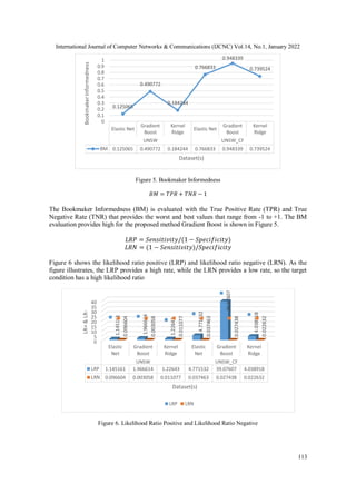
![International Journal of Computer Networks & Communications (IJCNC) Vol.14, No.1, January 2022
114
Diagnostic odds ratios (DORs) indicate a test's effectiveness. The LLR is defined as the ratio of
the probability of a positive test with an attack to the probability of a positive test without an
attack, as shown in Figure 7.
Figure 7. Diagnostic Odds Ratio (DOR)
5. CONCLUSION
This work introduces a framework for intrusion detection that deals with attack identification and
prediction using machine learning strategies in the UNSW-NB15 dataset. The proposed model
that employs the UNSW dataset for the attack prediction which includes the novel custom feature
derivation for the effective prediction is implemented. The model deals with both UNSW and
UNSW_CF features for the prediction using machine learning. The preprocessing phase is
employed to clean the raw dataset to avoid duplicate records, missing columns, and null values
from the dataset. The cleaned dataset is then analyzed to evaluate the custom features for the
prediction. This work uses feature selection strategies such as FPA and mRMR for
dimensionality reduction by selecting the most significant features which would increase the
accuracy of the prediction while detection. Then the classification techniques (EN, IGB, and
KRR) are applied to the significant feature subset for the attack detection. The performance
results show that the proposed technique IGB gives better results for performance metrics like
accuracy, error rate, sensitivity, specificity, DOR, LRP, and LRN. The framework would be
included with various algorithms for the exploration. Also, the framework can be extended with
the inclusion of different datasets and algorithms for enhancement.
CONFLICT OF INTEREST
The author declare no Conflicts of Interest.
REFERENCES
[1] T. A. Tchakoucht and M. Ezziyyani, (2018),“Building A Fast Intrusion Detection System For
HighSpeed- Building A Fast Intrusion Detection System For High-Speed- Networks : Probe and DoS
Attacks Detection”, In Proc. of the First International Conference On Intelligent Computing in Data
Sciences, Vol. 127, pp. 521–530.
0 500 1000 1500
Elastic Net
Kernel Ridge
Gradient Boost
UNSW
UNSW_
CF
DOR
DATASET(S)
UNSW UNSW_CF
Elastic
Net
Gradient
Boost
Kernel
Ridge
Elastic
Net
Gradient
Boost
Kernel
Ridge
DOR 11.85422643.0115110.7143127.36681424.161178.4576](https://image.slidesharecdn.com/14122cnc07-220219052953/85/AN-EFFICIENT-INTRUSION-DETECTION-SYSTEM-WITH-CUSTOM-FEATURES-USING-FPA-GRADIENT-BOOST-MACHINE-LEARNING-ALGORITHM-16-320.jpg)
![International Journal of Computer Networks & Communications (IJCNC) Vol.14, No.1, January 2022
115
[2] Moustafa, N., Slay, J., 2015, “Unsw-nb15: a comprehensive data set for network intrusion detection
systems (unsw-nb15 network data set)”, Military communications and information systems
conference (MilCIS), IEEE, pp. 1–6.
[3] F. A. Khan, A. Gumaei, A. Derhab, and A. Hussain, (2019), “TSDL: A two-stage deep learning
model for efficient network intrusion detection”, IEEE Access, Vol. 7, pp. 30373–30385.
[4] H. M. Anwer, M. Farouk, and A. Addel-Hamid, (2018), “A Framework for Efficient Network
Anomaly Intrusion Detection with Features Selection”, In: Proc. of the 9th International Conference
on Information and Communication Systems (ICICS), pp. 157–162.
[5] Khan NM, Negi A, Thaseen, (2018), “Analysis on improving the performance of machine learning
models using feature selection technique”, In: International conference on intelligent systems design
and applications, Springer, pp. 69–77.
[6] Zong W, Chow Y-W, Susilo W., (2018), “A two-stage classifier approach for network intrusion
detection”, International conference on information security practice and experience. Springer, pp.
329–340.
[7] Gao J, Chai S, Zhang B, Xia Y., (2019), “Research on network intrusion detection based on
incremental extreme learning machine and adaptive principal component analysis”, Energies 2019,
Vol. 12, No. 7.
[8] Sydney M. Kasongo and Yanxia Sun, (2020), “Performance Analysis of Intrusion Detection Systems
Using a Feature Selection Method on the UNSW-NB15 Dataset”, Journal of Big Data. Springer
Open, pp. 1-20.
[9] Toldinas, J. Venˇckauskas, A. Damaševiˇcius, R.; Grigaliunas, Š. Morkeviˇcius, N. Baranauskas, E.,
(2021), “A Novel Approach for Network Intrusion Detection Using Multistage Deep Learning Image
Recognition”, Electronics 2021, Vol. 10, No. 1854, https://doi.org/10.3390/ electronics10151854.
[10] Agarwal A, Sharma P, Alshehri M, Mohamed AA, Alfarraj O., (2021), “Classification model for
accuracy and intrusion detection using machine learning approach”, PeerJ Computer Science, DOI
10.7717/peerj-cs.437.
[11] Ahmad, M., Riaz, Q., Zeeshan, M., (2021), “Intrusion detection in the internet of things using
supervised machine learning based on application and transport layer features using UNSW-NB15
data-set”, Journal of Wireless Communication Network 2021, Vol. 10,
https://doi.org/10.1186/s13638-021-01893-8.
[12] D.V. Jeyanthi, Dr. B. Indrani, (2021), “Intrusion Detection System intensive on Securing IoT
Networking Environment based on Machine Learning Strategy”, Springer, Proceedings of the 5th
International Conference on Intelligent Data Communication Technologies and Internet of Things
(ICICI-2021).Lecture Notes on Data Engineering and Communications Technologies, DOI :
10.1007/978-981-16-7610-9
[13] Mousa Al-Akhras, Mohammed Alawairdhi1 Ali Alkoudari and Samer Atawneh, “using
machine learning to build a classification model for iot networks to detect attack signatures”,
International Journal of Computer Networks & Communications (IJCNC),
https://ijcnc.com/2020/12/12/ijcnc-07-15/
[14] Tran Hoang Hai, Le Huy Hoang, and Eui-nam Huh, (2020), “Network Anomaly Detection Based On
Late Fusion Of Several Machine Learning Algorithms”, International Journal of Computer Networks
& Communications (IJCNC), Vol.12, No.6, pp. 117-131, DOI: 10.5121/ijcnc.2020.12608
[15] Nour Moustafa and Jill Slay, “The evaluation of Network Anomaly Detection Systems: Statistical
analysis of the UNSW-NB15 data set and the comparison with the KDD99 data set” ,Information
Security Journal: A Global Perspective, Taylor & Francisdoi:10.1080/19393555.2015.1125974
AUTHORS
1. D.V. Jeyanthi, working as Assistant Professor in Department of Computer Science, Sourashtra
College, Madurai. Doing research work in Network Security and Intrusion Detection System.
2. Dr. B. Indrani ,working as Assistant Professor and Head(i/c) in Department of Computer Science in
DDE Section, Madurai Kamaraj Univerisity. Madurai. Highly interested in doing research in network
security, cryptography and big data. Has published various research papers in international scopus,
web of science, springer, referred journals.](https://image.slidesharecdn.com/14122cnc07-220219052953/85/AN-EFFICIENT-INTRUSION-DETECTION-SYSTEM-WITH-CUSTOM-FEATURES-USING-FPA-GRADIENT-BOOST-MACHINE-LEARNING-ALGORITHM-17-320.jpg)