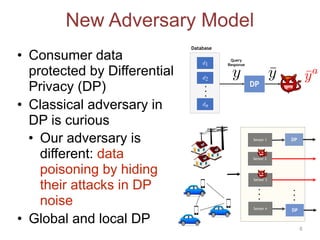
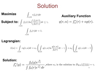
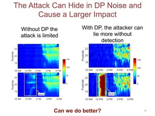
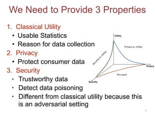
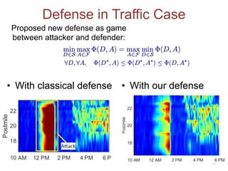
This document discusses adversarial classification under differential privacy. It proposes a new defense against adversarial distributions that aims to provide utility, privacy, and security. The defense frames the problem as a game between an attacker and defender. The defender first designs a classifier to minimize errors while satisfying privacy constraints. The attacker then tries to maximize damage by poisoning the data. 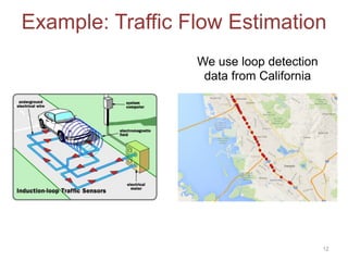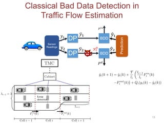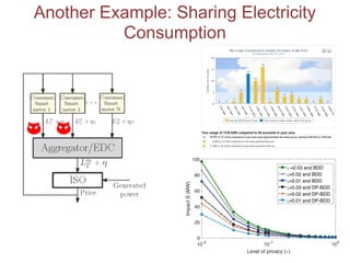The proposed defense can outperform classical defenses by allowing the defender to certify performance guarantees no matter the attacker's strategy, improving on approaches that are limited once the attacker adapts. Examples applying this defense to traffic flow estimation and electricity consumption data are also discussed.

1. Adversarial Classification Under
Differential Privacy
Jairo Giraldo
University of Utah
Alvaro A. Cardenas
UC Santa Cruz
Murat Kantarcioglu
UT Dallas
Jonathan Katz
GMU

2. Kevin Ashton (British
entrepreneur) coined
the term IoT in 1999.
2
• 20th Century: computers were
brains without senses—-they
only knew what we told them.
• More info in the world than what
people can type on keyboard
• 21st century: computers sense
things, e.g., GPS we take for
granted in our phones

3. New Privacy Concerns
3

4. In Addition to Privacy, There is Another Problem:
Data Trustworthiness
4

5. Privacy
Security
Utility
This work
Privacy vs. Utility
We Need to Provide 3 Properties
1. Classical Utility
• Usable Statistics
• Reason for data collection
2. Privacy
• Protect consumer data
3. Security
• Trustworthy data
• Detect data poisoning
• Different from classical utility because this
is an adversarial setting
5

6. DP
𝑑1
𝑑2
𝑑𝑛
Database
Query
Response
DP
DP
Sensor 1
Sensor 2
Sensor 3
Sensor n
New Adversary Model
• Consumer data
protected by Differential
Privacy (DP)
• Classical adversary in
DP is curious
• Our adversary is
different: data
poisoning by hiding
their attacks in DP
noise
• Global and local DP
6

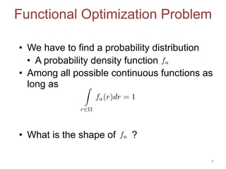
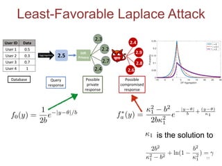
7. Adversary Goals
• Intelligently poison the data in a way that is
hard to detect (hide attack in DP noise)
• Achieve maximum damage to the utility of the
system (deviate estimate as much as possible)
7
max
fa
E[Y a
]
s.t.
DKL(fakf0) 
fa 2 F
Classical DP
Attack Goals:
Multi-criteria Optimization
¯Y M(D)
¯Y ⇠ f0
Attack
Y a
instead of ¯Y

8. Functional Optimization Problem
• We have to find a probability distribution
• A probability density function
• Among all possible continuous functions as
long as
• What is the shape of ?
8
fa
Z
r2⌦
fa(r)dr = 1
fa

9. Solution: Variational Methods
• Variational methods are a useful tool to find
the shape of functions or the structure of
matrices
• They replace the function or matrix
optimization problem with a parameterized
perturbation of the function or matrix
• We can then optimize with respect to the
parameter to find the “shape” of the function/
matrix
• The Lagrange multipliers give us the final
parameters of the function
9

10. Solution
10
Z
r2⌦
rfa(r)dr
Z
r2⌦
fa(r) ln
✓
fa(r)
f0(r)
◆
dr  .
Z
r2⌦
fa(r)dr = 1.
Maximize
Subject to: q(r, ↵) = f⇤
a (r) + ↵p(r).
Auxiliary Function
Lagrangian:
Solution:
L(↵) =
Z
r2⌦
rq(r, ↵)dr + 1
0
@
Z
r2⌦
q(r, ↵) ln
q(r, ↵)
f0(r)
dr
1
A + 2
0
@
Z
r2⌦
q(r, ↵)dr 1
1
A
f⇤
a (y) =
f0(y)e
y
1
R
f0(r)e
r
1 dr
,where 1 is the solution to DKL(f⇤
a kf0) = .

11. Least-Favorable Laplace Attack
11
User ID Data
User 1 0.5
User 2 0.3
User 3 0.7
User 4 1
2.5
Diff.
Privacy
2.3
2.2
2.7
2.4
2.4
2.9
2.8
2.6
Database Query
response
Possible
private
response
Possible
compromised
response
Aggregation
f0(y) =
1
2b
e |y ✓|/b
f⇤
a (y) =
2
1 b2
2b2
1
e
|y ✓|
b +
(y ✓)
1
2b2
2
1 b2
+ ln(1
b2
2
1
) =
1 is the solution to
-10 -5 0 5 10 15 20 25 30
DP Aggregation
0
0.05
0.1
0.15
0.2
0.25
Probability
= 0
= 0.1
= 2

12. Example: Traffic Flow Estimation
12
-Vehicle count
- Occupancy
We use loop detection
data from California

13. Classical Bad Data Detection in
Traffic Flow Estimation
13
Sensor
Readings
DP
BDD
BDD
DP
Prediction
ˆyi(k + 1) = ˆyi(k) +
T
li
✓
li 1
li
Fin
i (k)
Fout
i (k) + Qi(yi(k) ˆyi(k))
Cabinet
TMC
Fout
i (k)Fin
i (k)
Li+1
Cell i 1 Cell i Cell i + 1
i 1 = 3
Loop
detector

14. The Attack Can Hide in DP Noise and
Cause a Larger Impact
14
Without DP the
attack is limited
With DP, the attacker can
lie more without
detection
Can we do better?

15. Defense Against Adversarial (Adaptive)
Distributions
•Player 1 designs classifier D ∈ S minimize Φ(D,A) (e.g.,
Pr[Miss Detection] Subject to fix false alarms)
-Player 1 makes the first move
•Player 2 (attacker) has multiple strategies A∈ F
-Makes the move after observing the move of the classifier
•Player 1 wants provable performance guarantees:
-Once it selects Do by minimizing Φ, it wants proof that no matter what
the attacker does, Φ<m, i.e.
•
15

16. Defense in Traffic Case
• With classical defense
16
Proposed new defense as game
between attacker and defender:
• With our defense

17. Another Example: Sharing Electricity
Consumption
17
10-2
10-1
100
Level of privacy ( )
0
20
40
60
80
100
ImpactS(MW)
=0.03 and BDD
=0.02 and BDD
=0.01 and BDD
=0.03 and DP-BDD
=0.02 and DP-BDD
=0.01 and DP-BDD

18. Conclusions
• Growing number of applications where we
need to provide utility, privacy, and security
• In particular, adversarial classification
under differential privacy
• Various possible extensions
• Different quantification of privacy loss
(e.g., Rényi DP)
• Adversary models (noiseless privacy), etc.
• Related work on DP and adversarial ML
• Certified robustness
18