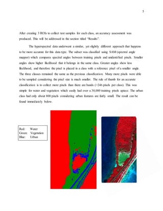
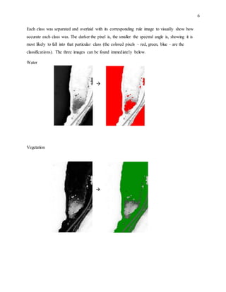
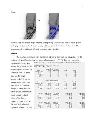
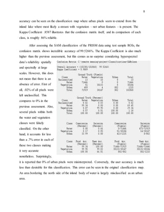
SlideShare a Scribd company logo
1
Jeffrey Schorsch
April 19, 2016
Remote Sensing Data Analysis:
Hyperspectral vs. Multispectral
Introduction
Choosing the most effective data for any given remote sensing project is not always the
simplest decision. The decision is made based off of many different factors depending on cost,
timeframe to collect data, the strengths and weaknesses of each sensor type, and so on. While
this report does not go into great detail about the cost and specific time to acquire datasets, these
factors will not be ignored. This report focuses on the strengths and weaknesses of two very
different types of data, hyperspectral and multispectral, in an attempt to answer one question:
why should we choose one over the other when analyzing land cover features? There is no
specific answer to this question, but strengths and weaknesses of each type will be weighed to
find out which one is more effective for the given project. The goal of this report is to inform
amateur researchers about the proper ways to utilize each form of data to reach the best results
possible for any given project.
Background
Multispectral and hyperspectral data was compared using classification and data analysis
methods in ENVI. These data sets differ in resolution spatially, spectrally, and radiometric. This
is what will inevitably affect how accurate each data set is at a large scale and small scale for
land cover classification and analysis. For example, Landsat 8 imagery (used in this project) has
a spatial resolution of 30x30 m. While it is effective at distinguishing various land covers at a
small scale, it is less effective at distinguishing smaller, individual features primarily identified at
a much larger scale (Qihao et al. 2008). Portable Remote Imaging Spectrometer, or PRISM,
(exclusively used in this project for hyperspectral data) has a spatial resolution of .9x.9 m.
Already a stark difference can be seen between each dataset’s spatial resolutions. The smaller
pixel size allows researchers to distinguish and analyze different features that would otherwise
be combined into one ambiguous pixel in multispectral data. The tradeoff for having such a high
spatial resolution means that it can never be used for small scale analysis that Landsat 8 is used
2
for. This could only be achieved if the researcher is willing to acquire many datasets of
hyperspectral scenes which can be costly, timely, and difficult to work with.
Qihao et al. (2008) compared the spectral resolutions using both datasets to observe urban
and environmental landscapes. It was regarded that multispectral data did not have a high enough
spectral resolution to be reliable when observing urban features, and hyperspectral data was
recommended. Though multispectral data does not have a spectral resolution as fine as
hyperspectral does not mean it is not useful. Li et al. (2016) found success using multispectral
data when classifying tropical savannahs. Multispectral images are generally only comprised of 6
bands between 450-2350 nm wavelengths and an additional thermal band beyond that scope.
When coupled with various analyzing techniques like NDVI as well as a researcher’s knowledge
of the observed area, multispectral data is very useful and accurate at classifying large
landscapes more efficiently than hyperspectral. On the other hand, hyperspectral data has a fine
spectral resolution useful for classifying smaller features, especially urban. PRISM data consists
of 246 bands between 350-1045 nm that allow researchers to identify features without needing
prior knowledge of the given area. The disadvantage of this data is the weak differentiation of
low-albedo objects. Hundreds of detected wavelengths per .9x.9m pixel can lead to random noise
that may affect the measurability of a given pixel, which can be seen later in the results. This also
makes datasets massive in storage size (roughly 8 GB) and costly to acquire in quantities.
The last factor to compare is radiometric resolution. The Landsat 8 sensor collects data
around a 12-bit range. This means that each band is translated into 4,096 grey scale levels. This
is a greater bit depth in comparison to older Landsat products (Landsat, 2015). PRISM data
boasts a bit depth of 14 with over 16,000 gray scales levels (PRISM, 2015). In simpler terms, the
higher the bit depth a sensor has the wider the range of values each pixel has. This allows
observers to perceive greater differences in reflective values for each pixel; therefore containing
more information than one that has a lower bit depth. It would be easy to say that hyperspectral,
with a bit depth of 14, has a greater radiometric resolution than Landsat 8 with a bit depth of 12.
However, this is not entirely true considering that this resolution is affected by noise. As
discussed earlier, hyperspectral data’s small pixel size can make it easily affected by random
noise across 246 bands. This makes the two data products difficult to compare in terms of
3
radiometric resolution and should be weighed by each dataset’s advantages and disadvantages
toward the given observed area.
Data Analyzed
The multispectral data analyzed in this project consisted of the southern coast of Florida
and almost the entirety of the Florida Keys. The hyperspectral data consisted of a narrow scene
stretching vertically across the island of Long Key in the Florida Keys. Both of the multispectral
and hyperspectral data were subset into a scene of Long Key roughly 1.1 square km
(24°48'45.2"N, 80°49'47.6"W). The multispectral data was set to red band = 865 nm, green band
= 655 nm, and blue band = 561 nm. The hyperspectral data was set to similar bands for the most
accurate comparison: red band = 860 nm, green band = 650 nm, and blue band = 562 nm. This
created two CIR subsets of Long Key.
Method
After this initial setup was completed there was a hyperspectral subset and multispectral
subset equal in both dimension and area. As discussed in the section titled “Background”, the
multispectral subset was very pixelated due to having a lower spatial resolution than
hyperspectral. The hyperspectral subset remained very clear and features remained fairly
distinguishable. The two subsets were set to nearly equal band combinations but came from
different sensors and therefore have differing spatial, spectral, and radiometric resolutions
naturally. This can result in slightly differing data values in each subset. This would lead to bias
in the final classification results unless corrected. Nevertheless, this bias was nearly impossible
to avoid. The multispectral subset went through a radiometric calibration to correct for this bias.
However, the hyperspectral subset was missing gain and offset values for the same calibration.
After a bit of research, the values could not be found, but there was a passage on the PRISM
website that explained that the data already went through radiometric calibration. This may lead
to a slight bias considering the process was not verified as going through the exact same
calibration as the multispectral subset to ensure a bias-free result.
Visually, the two subsets were set to Linear 2% and it seemed they portrayed the same
reflectance values overall disregarding the massive spatial resolution difference. Two samples of
the subsets can be seen immediately below (left: hyperspectral, right: multispectral).
4
The two original subsets these samples were derived from were used to create classification
schemes to further compare their effectiveness in large scale use.
Supervised classification was performed on the multispectral subset. Training samples
were collected in three different classes: water, vegetation, and urban. Due to limited pixels to
classify, water training samples were limited to 73, vegetation to 40, and urban to 21. These low
sample sizes reluctantly did not seem to have any particular impact on the classification’s
accuracy. The resulting classification map can be seen immediately below.
Red: Water
Green: Vegetation
Blue: Urban
5
After creating 3 ROIs to collect test samples for each class, an accuracy assessment was
produced. This will be addressed in the section titled “Results”.
The hyperspectral data underwent a similar, yet slightly different approach that happens
to be more accurate for this data type. The subset was classified using SAM (spectral angle
mapper) which compares spectral angles between training pixels and unidentified pixels. Smaller
angles show higher likelihood that it belongs in the same class. Greater angles show less
likelihood, and therefore the pixel is placed in a class with a reference pixel of a smaller angle.
The three classes remained the same as the previous classification. Many more pixels were able
to be sampled considering the pixel size is much smaller. The rule of thumb for an accurate
classification is to collect more pixels than there are bands (>246 pixels per class). This was
simple for water and vegetation which easily had over a 30,000 training pixels apiece. The urban
class had only about 800 pixels considering urban features are fairly small. The result can be
found immediately below.
Red: Water
Green: Vegetation
Blue: Urban
6
Each class was separated and overlaid with its corresponding rule image to visually show how
accurate each class was. The darker the pixel is, the smaller the spectral angle is, showing it is
most likely to fall into that particular class (the colored pixels – red, green, blue – are the
classifications). The three images can be found immediately below.
Water

Vegetation

7
Urban

It can be seen that the rule images and their corresponding classifications seem to match up well
portraying an accurate classification. Again, 3 ROIs were created to collect test samples. This
assessment will be addressed below in the section titled “Results”.
Results
The accuracy assessments were much more impressive than what was anticipated. For the
multispectral classification, there was an overall accuracy of 91.7910%. This was a successful
result considering the low
sample size of pixels and the
medium spatial resolution of
Landsat 8 data. The urban
class has the lowest
accuracy, 52.38%, but this
was expected. 30m x 30m
pixel size is not sufficient
enough to detect individual
urban features, and therefore
pixels project weighted
values of the features
contained within them – in
this case, both urban and
vegetation features. This low
8
accuracy can be seen on the classification map where urban pixels seem to extend from the
inland lake where most likely a stream with vegetation – not urban features – is present. The
Kappa Coefficient .8587 illustrates that the confusion matrix itself, and its comparison of each
class, is roughly 86% reliable.
After assessing the SAM classification of the PRISM data using test sample ROIs, the
confusion matrix shows incredible accuracy of 99.5266%. The Kappa Coefficient is also much
higher than the previous assessment, but this comes as no surprise considering hyperspectral
data’s reliability spatially
and spectrally at large
scales. However, this does
not mean that there is an
absence of error. First of
all, .02% of all pixels were
left unclassified. This
compares to 0% in the
previous assessment. Also,
several pixels within both
the water and vegetation
classes were falsely
classified. On the other
hand, it accounts for less
than a .7% error in each of
these two classes making
it very accurate
nonetheless. Surprisingly,
it is reported that 0% of urban pixels were misinterpreted. Conversely, the user accuracy is much
less than desirable for this classification. This error can be seen in the original classification map.
An area bordering the north side of the inland body of water is largely misclassified as an urban
area.
9
This error can be explained by hyperspectral data’s noise interference discussed in the
section titled “Background”. Both urban and shallow water features in some cases have similar
reflectance values making it difficult for SAM to pick up these subtle differences. The sensor is
detecting 246 wavelengths per pixel, and therefore random noise can slightly affect the data
value of the pixels. For example, sand on the road is reflecting values similar to that of sand
detected in shallow water. The 246 bands are detecting urban signatures along with sand, just as
it is detecting water signatures along with sand. The sand in this situation can be seen as the
noise that affects the value of the pixel. The only way to adjust for this issue would be to use
more classes. Depending on the heterogonous spectral variability of the landscape, more or less
classes should be used. In this situation at least 6 classes could have been used; it was fixed at 3
just to show its effectiveness compared to 3 classes in multispectral classification. Multispectral
data only detects 8 bands, so the pixels are not projecting this noise at nearly the same
magnitude. It is only detecting the dominate feature in that wavelength – which in this case is the
road or the water. The multispectral classification still confused several pixels for urban features,
but this is most likely due to the low spatial resolution leading to pixels seeming too ambiguous
to classify.
Conclusion
The choice of whether to use hyperspectral or multispectral data (or even something
between the two) depends on the landscape and its scale, and the judgment of the researcher.
Hyperspectral data is efficient at classifying and distinguishing features at a large scale. Its pixel
size is small, whereas multispectral data’s spatial resolution often combines multiple features
into one pixel. A SAM classification – like this one – is quite smooth on a large scale over the
coarseness of the multispectral classification. At a small scale, hyperspectral is nearly useless.
Imagine observing the entire Florida Keys (instead of a section of one island), it would take tens
maybe hundreds of scenes to complete. This would inevitably be too costly, too timely to work
with, too massive for hard-drive space, and all the data may not even be available for download.
Also, at a larger scale, the landscape becomes much more homogenous making it more effective
for satellite data like Landsat 8 to be utilized. Urban areas would be almost undetectable, while
vegetation, shorelines, and water bodies become easier to differentiate. In many ways, the scale
of the landscape helps decide which sensor type is most effective. Lastly, one advantage
hyperspectral has is the amount of data stored within the scene. This allows for the researcher to
10
have almost no knowledge of the given area and still be able to classify it correctly. Multispectral
takes a bit more knowledge to distinguish minute features amongst the broad landscapes (ie.
various kinds of tree covers, or urban areas) that may not be so clear.
While it may seem this report was strictly trying to weigh the advantages and
disadvantages of each data type to help guide decisions; this is not entirely the point. Much of
these decisions come down to common sense depending on the landscape scale and the scope of
the project. The scale of each data type is so immensely different that usually there is not much
need for a decision at all. The true purpose was to analyze each data type in order to illustrate its
effectiveness overall so that amateur researchers, like myself, understand the different data
sources available for use, how radiometric, spatial, and spectral resolutions affect research
results, and by what methods to utilize this data properly. These kinds of questions can all be
answered by presenting the information as a decision for the researcher, rather than a bulk of
directionless information.
11
References
Landsat 8. (2015). Retrieved April 17, 2016, from http://landsat.usgs.gov/landsat8.php
Li, Z., & Guo, X. (2016). Remote sensing of terrestrial non-photosynthetic vegetation using
hyperspectral, multispectral, SAR, and LiDAR data. Progress In Physical
Geography, 40(2), 276-304. doi:10.1177/0309133315582005.
PRISM website: Instrument. (2015). Retrieved April 17, 2016, from http://prism.jpl.nasa.gov
/instrument.html.
Qihao, W., Xuefei, H., & Dengsheng, L. (2008). Extracting impervious surfaces from spatial
resolution multispectral and hyperspectral imagery: a comparison. International Journal
Of Remote Sensing, 29(11), 3209-3232. doi:10.1080/01431160701469024medium.
I have neither given or received, nor have I tolerated others’ use of unauthorized aid.

More Related Content

What's hot

Remote sensing e course (Geohydrology)
Remote sensing e course (Geohydrology)Remote sensing e course (Geohydrology)
Remote sensing e course (Geohydrology)
Fatwa Ramdani
 
NDVI
NDVINDVI
TWO LEVEL DATA FUSION MODEL FOR DATA MINIMIZATION AND EVENT DETECTION IN PERI...
TWO LEVEL DATA FUSION MODEL FOR DATA MINIMIZATION AND EVENT DETECTION IN PERI...TWO LEVEL DATA FUSION MODEL FOR DATA MINIMIZATION AND EVENT DETECTION IN PERI...
TWO LEVEL DATA FUSION MODEL FOR DATA MINIMIZATION AND EVENT DETECTION IN PERI...
pijans
 
Scale and resolution
Scale and resolutionScale and resolution
Scale and resolution
shabir dar
 
Chapter 5: Remote sensing
Chapter 5: Remote sensingChapter 5: Remote sensing
Chapter 5: Remote sensing
Shankar Gangaju
 
The single image dehazing based on efficient transmission estimation
The single image dehazing based on efficient transmission estimationThe single image dehazing based on efficient transmission estimation
The single image dehazing based on efficient transmission estimation
AVVENIRE TECHNOLOGIES
 
study and analysis of hy si data in 400 to 500
study and analysis of hy si data in 400 to 500study and analysis of hy si data in 400 to 500
study and analysis of hy si data in 400 to 500
IJAEMSJORNAL
 
Energy aware model for sensor network a nature inspired algorithm approach
Energy aware model for sensor network  a nature inspired algorithm approachEnergy aware model for sensor network  a nature inspired algorithm approach
Energy aware model for sensor network a nature inspired algorithm approach
ijdms
 

What's hot (8)

Remote sensing e course (Geohydrology)
Remote sensing e course (Geohydrology)Remote sensing e course (Geohydrology)
Remote sensing e course (Geohydrology)
 
NDVI
NDVINDVI
NDVI
 
TWO LEVEL DATA FUSION MODEL FOR DATA MINIMIZATION AND EVENT DETECTION IN PERI...
TWO LEVEL DATA FUSION MODEL FOR DATA MINIMIZATION AND EVENT DETECTION IN PERI...TWO LEVEL DATA FUSION MODEL FOR DATA MINIMIZATION AND EVENT DETECTION IN PERI...
TWO LEVEL DATA FUSION MODEL FOR DATA MINIMIZATION AND EVENT DETECTION IN PERI...
 
Scale and resolution
Scale and resolutionScale and resolution
Scale and resolution
 
Chapter 5: Remote sensing
Chapter 5: Remote sensingChapter 5: Remote sensing
Chapter 5: Remote sensing
 
The single image dehazing based on efficient transmission estimation
The single image dehazing based on efficient transmission estimationThe single image dehazing based on efficient transmission estimation
The single image dehazing based on efficient transmission estimation
 
study and analysis of hy si data in 400 to 500
study and analysis of hy si data in 400 to 500study and analysis of hy si data in 400 to 500
study and analysis of hy si data in 400 to 500
 
Energy aware model for sensor network a nature inspired algorithm approach
Energy aware model for sensor network  a nature inspired algorithm approachEnergy aware model for sensor network  a nature inspired algorithm approach
Energy aware model for sensor network a nature inspired algorithm approach
 

Viewers also liked

project report on REMOTE SENSING THERMOMETER
project report on REMOTE SENSING THERMOMETERproject report on REMOTE SENSING THERMOMETER
project report on REMOTE SENSING THERMOMETER
dreamervikas
 
Remote Sensing PPT
Remote Sensing PPTRemote Sensing PPT
Remote Sensing PPT
Amal Murali
 
1. medico kitchen plants By Allah Dad Khan
1. medico kitchen plants By Allah Dad Khan 1. medico kitchen plants By Allah Dad Khan
1. medico kitchen plants By Allah Dad Khan
Mr.Allah Dad Khan
 
Cynthia Crawford Resume
Cynthia Crawford ResumeCynthia Crawford Resume
Cynthia Crawford Resume
Cyndi Crawford
 
Certificate_1
Certificate_1Certificate_1
Certificate_1
Bilal Ahmed
 
Resume9-30-15
Resume9-30-15Resume9-30-15
Resume9-30-15
Claude Ruboneka
 
Tom Bastiman Portfolio
Tom Bastiman PortfolioTom Bastiman Portfolio
Tom Bastiman Portfolio
Tom Bastiman
 
Cover Letter + Resume
Cover Letter + ResumeCover Letter + Resume
Cover Letter + Resume
Louis A. Hermansen
 
Pro con which witch
Pro con which witchPro con which witch
Pro con which witch
Bruce Alldis
 
Designing for Sleep Surface Breathability to Save Infant Lives
Designing for Sleep Surface Breathability to Save Infant LivesDesigning for Sleep Surface Breathability to Save Infant Lives
Designing for Sleep Surface Breathability to Save Infant Lives
Dave Karow
 
Ley denuncias y recompensas Defraudación Tributaria anteproyecto por uak al 2...
Ley denuncias y recompensas Defraudación Tributaria anteproyecto por uak al 2...Ley denuncias y recompensas Defraudación Tributaria anteproyecto por uak al 2...
Ley denuncias y recompensas Defraudación Tributaria anteproyecto por uak al 2...
EXPAUK
 
Acurea costas costos enero2016 img170
Acurea costas costos enero2016 img170Acurea costas costos enero2016 img170
Acurea costas costos enero2016 img170
EXPAUK
 
REMOTE SENSING
REMOTE SENSINGREMOTE SENSING
REMOTE SENSING
KANNAN
 

Viewers also liked (13)

project report on REMOTE SENSING THERMOMETER
project report on REMOTE SENSING THERMOMETERproject report on REMOTE SENSING THERMOMETER
project report on REMOTE SENSING THERMOMETER
 
Remote Sensing PPT
Remote Sensing PPTRemote Sensing PPT
Remote Sensing PPT
 
1. medico kitchen plants By Allah Dad Khan
1. medico kitchen plants By Allah Dad Khan 1. medico kitchen plants By Allah Dad Khan
1. medico kitchen plants By Allah Dad Khan
 
Cynthia Crawford Resume
Cynthia Crawford ResumeCynthia Crawford Resume
Cynthia Crawford Resume
 
Certificate_1
Certificate_1Certificate_1
Certificate_1
 
Resume9-30-15
Resume9-30-15Resume9-30-15
Resume9-30-15
 
Tom Bastiman Portfolio
Tom Bastiman PortfolioTom Bastiman Portfolio
Tom Bastiman Portfolio
 
Cover Letter + Resume
Cover Letter + ResumeCover Letter + Resume
Cover Letter + Resume
 
Pro con which witch
Pro con which witchPro con which witch
Pro con which witch
 
Designing for Sleep Surface Breathability to Save Infant Lives
Designing for Sleep Surface Breathability to Save Infant LivesDesigning for Sleep Surface Breathability to Save Infant Lives
Designing for Sleep Surface Breathability to Save Infant Lives
 
Ley denuncias y recompensas Defraudación Tributaria anteproyecto por uak al 2...
Ley denuncias y recompensas Defraudación Tributaria anteproyecto por uak al 2...Ley denuncias y recompensas Defraudación Tributaria anteproyecto por uak al 2...
Ley denuncias y recompensas Defraudación Tributaria anteproyecto por uak al 2...
 
Acurea costas costos enero2016 img170
Acurea costas costos enero2016 img170Acurea costas costos enero2016 img170
Acurea costas costos enero2016 img170
 
REMOTE SENSING
REMOTE SENSINGREMOTE SENSING
REMOTE SENSING
 

Similar to Advanced Remote Sensing Project Report

IGARSS 2011 Arch.ppt
IGARSS 2011 Arch.pptIGARSS 2011 Arch.ppt
IGARSS 2011 Arch.ppt
grssieee
 
IGARSS 2011.ppt
IGARSS 2011.pptIGARSS 2011.ppt
IGARSS 2011.ppt
grssieee
 
IGARSS 2011.ppt
IGARSS 2011.pptIGARSS 2011.ppt
IGARSS 2011.ppt
grssieee
 
ARCHAEOLOGICAL LAND USE CHARACTERIZATION USING MULTISPECTRAL REMOTE SENSING DATA
ARCHAEOLOGICAL LAND USE CHARACTERIZATION USING MULTISPECTRAL REMOTE SENSING DATAARCHAEOLOGICAL LAND USE CHARACTERIZATION USING MULTISPECTRAL REMOTE SENSING DATA
ARCHAEOLOGICAL LAND USE CHARACTERIZATION USING MULTISPECTRAL REMOTE SENSING DATA
grssieee
 
IGARSS 2011.ppt
IGARSS 2011.pptIGARSS 2011.ppt
IGARSS 2011.ppt
grssieee
 
IGARSS 2011.ppt
IGARSS 2011.pptIGARSS 2011.ppt
IGARSS 2011.ppt
grssieee
 
IGARSS 2011.ppt
IGARSS 2011.pptIGARSS 2011.ppt
IGARSS 2011.ppt
grssieee
 
IGARSS 2011.ppt
IGARSS 2011.pptIGARSS 2011.ppt
IGARSS 2011.ppt
grssieee
 
IGARSS 2011.ppt
IGARSS 2011.pptIGARSS 2011.ppt
IGARSS 2011.ppt
grssieee
 
IGARSS 2011.ppt
IGARSS 2011.pptIGARSS 2011.ppt
IGARSS 2011.ppt
grssieee
 
ARCHAEOLOGICAL LAND USE CHARACTERIZATION USING MULTISPECTRAL REMOTE SENSING DATA
ARCHAEOLOGICAL LAND USE CHARACTERIZATION USING MULTISPECTRAL REMOTE SENSING DATAARCHAEOLOGICAL LAND USE CHARACTERIZATION USING MULTISPECTRAL REMOTE SENSING DATA
ARCHAEOLOGICAL LAND USE CHARACTERIZATION USING MULTISPECTRAL REMOTE SENSING DATA
grssieee
 
IGARSS 2011.ppt
IGARSS 2011.pptIGARSS 2011.ppt
IGARSS 2011.ppt
grssieee
 
ARCHAEOLOGICAL LAND USE CHARACTERIZATION USING MULTISPECTRAL REMOTE SENSING DATA
ARCHAEOLOGICAL LAND USE CHARACTERIZATION USING MULTISPECTRAL REMOTE SENSING DATAARCHAEOLOGICAL LAND USE CHARACTERIZATION USING MULTISPECTRAL REMOTE SENSING DATA
ARCHAEOLOGICAL LAND USE CHARACTERIZATION USING MULTISPECTRAL REMOTE SENSING DATA
grssieee
 
IGARSS 2011.ppt
IGARSS 2011.pptIGARSS 2011.ppt
IGARSS 2011.ppt
grssieee
 
Super-Resolution of Multispectral Images
Super-Resolution of Multispectral ImagesSuper-Resolution of Multispectral Images
Super-Resolution of Multispectral Images
ijsrd.com
 
COLOUR IMAGE REPRESENTION OF MULTISPECTRAL IMAGE FUSION
COLOUR IMAGE REPRESENTION OF MULTISPECTRAL IMAGE FUSION COLOUR IMAGE REPRESENTION OF MULTISPECTRAL IMAGE FUSION
COLOUR IMAGE REPRESENTION OF MULTISPECTRAL IMAGE FUSION
acijjournal
 
COLOUR IMAGE REPRESENTION OF MULTISPECTRAL IMAGE FUSION
COLOUR IMAGE REPRESENTION OF MULTISPECTRAL IMAGE FUSIONCOLOUR IMAGE REPRESENTION OF MULTISPECTRAL IMAGE FUSION
COLOUR IMAGE REPRESENTION OF MULTISPECTRAL IMAGE FUSION
acijjournal
 
Hyperspectral Data Compression Using Spatial-Spectral Lossless Coding Technique
Hyperspectral Data Compression Using Spatial-Spectral Lossless Coding TechniqueHyperspectral Data Compression Using Spatial-Spectral Lossless Coding Technique
Hyperspectral Data Compression Using Spatial-Spectral Lossless Coding Technique
CSCJournals
 
Hyperparameters analysis of long short-term memory architecture for crop cla...
Hyperparameters analysis of long short-term memory  architecture for crop cla...Hyperparameters analysis of long short-term memory  architecture for crop cla...
Hyperparameters analysis of long short-term memory architecture for crop cla...
IJECEIAES
 
Hyperspectral & Remote Sensing on Remote Sensing and GIS.pptx
Hyperspectral & Remote Sensing on Remote Sensing and GIS.pptxHyperspectral & Remote Sensing on Remote Sensing and GIS.pptx
Hyperspectral & Remote Sensing on Remote Sensing and GIS.pptx
KabaliVasudevasu
 

Similar to Advanced Remote Sensing Project Report (20)

IGARSS 2011 Arch.ppt
IGARSS 2011 Arch.pptIGARSS 2011 Arch.ppt
IGARSS 2011 Arch.ppt
 
IGARSS 2011.ppt
IGARSS 2011.pptIGARSS 2011.ppt
IGARSS 2011.ppt
 
IGARSS 2011.ppt
IGARSS 2011.pptIGARSS 2011.ppt
IGARSS 2011.ppt
 
ARCHAEOLOGICAL LAND USE CHARACTERIZATION USING MULTISPECTRAL REMOTE SENSING DATA
ARCHAEOLOGICAL LAND USE CHARACTERIZATION USING MULTISPECTRAL REMOTE SENSING DATAARCHAEOLOGICAL LAND USE CHARACTERIZATION USING MULTISPECTRAL REMOTE SENSING DATA
ARCHAEOLOGICAL LAND USE CHARACTERIZATION USING MULTISPECTRAL REMOTE SENSING DATA
 
IGARSS 2011.ppt
IGARSS 2011.pptIGARSS 2011.ppt
IGARSS 2011.ppt
 
IGARSS 2011.ppt
IGARSS 2011.pptIGARSS 2011.ppt
IGARSS 2011.ppt
 
IGARSS 2011.ppt
IGARSS 2011.pptIGARSS 2011.ppt
IGARSS 2011.ppt
 
IGARSS 2011.ppt
IGARSS 2011.pptIGARSS 2011.ppt
IGARSS 2011.ppt
 
IGARSS 2011.ppt
IGARSS 2011.pptIGARSS 2011.ppt
IGARSS 2011.ppt
 
IGARSS 2011.ppt
IGARSS 2011.pptIGARSS 2011.ppt
IGARSS 2011.ppt
 
ARCHAEOLOGICAL LAND USE CHARACTERIZATION USING MULTISPECTRAL REMOTE SENSING DATA
ARCHAEOLOGICAL LAND USE CHARACTERIZATION USING MULTISPECTRAL REMOTE SENSING DATAARCHAEOLOGICAL LAND USE CHARACTERIZATION USING MULTISPECTRAL REMOTE SENSING DATA
ARCHAEOLOGICAL LAND USE CHARACTERIZATION USING MULTISPECTRAL REMOTE SENSING DATA
 
IGARSS 2011.ppt
IGARSS 2011.pptIGARSS 2011.ppt
IGARSS 2011.ppt
 
ARCHAEOLOGICAL LAND USE CHARACTERIZATION USING MULTISPECTRAL REMOTE SENSING DATA
ARCHAEOLOGICAL LAND USE CHARACTERIZATION USING MULTISPECTRAL REMOTE SENSING DATAARCHAEOLOGICAL LAND USE CHARACTERIZATION USING MULTISPECTRAL REMOTE SENSING DATA
ARCHAEOLOGICAL LAND USE CHARACTERIZATION USING MULTISPECTRAL REMOTE SENSING DATA
 
IGARSS 2011.ppt
IGARSS 2011.pptIGARSS 2011.ppt
IGARSS 2011.ppt
 
Super-Resolution of Multispectral Images
Super-Resolution of Multispectral ImagesSuper-Resolution of Multispectral Images
Super-Resolution of Multispectral Images
 
COLOUR IMAGE REPRESENTION OF MULTISPECTRAL IMAGE FUSION
COLOUR IMAGE REPRESENTION OF MULTISPECTRAL IMAGE FUSION COLOUR IMAGE REPRESENTION OF MULTISPECTRAL IMAGE FUSION
COLOUR IMAGE REPRESENTION OF MULTISPECTRAL IMAGE FUSION
 
COLOUR IMAGE REPRESENTION OF MULTISPECTRAL IMAGE FUSION
COLOUR IMAGE REPRESENTION OF MULTISPECTRAL IMAGE FUSIONCOLOUR IMAGE REPRESENTION OF MULTISPECTRAL IMAGE FUSION
COLOUR IMAGE REPRESENTION OF MULTISPECTRAL IMAGE FUSION
 
Hyperspectral Data Compression Using Spatial-Spectral Lossless Coding Technique
Hyperspectral Data Compression Using Spatial-Spectral Lossless Coding TechniqueHyperspectral Data Compression Using Spatial-Spectral Lossless Coding Technique
Hyperspectral Data Compression Using Spatial-Spectral Lossless Coding Technique
 
Hyperparameters analysis of long short-term memory architecture for crop cla...
Hyperparameters analysis of long short-term memory  architecture for crop cla...Hyperparameters analysis of long short-term memory  architecture for crop cla...
Hyperparameters analysis of long short-term memory architecture for crop cla...
 
Hyperspectral & Remote Sensing on Remote Sensing and GIS.pptx
Hyperspectral & Remote Sensing on Remote Sensing and GIS.pptxHyperspectral & Remote Sensing on Remote Sensing and GIS.pptx
Hyperspectral & Remote Sensing on Remote Sensing and GIS.pptx
 

Advanced Remote Sensing Project Report

  • 1. 1 Jeffrey Schorsch April 19, 2016 Remote Sensing Data Analysis: Hyperspectral vs. Multispectral Introduction Choosing the most effective data for any given remote sensing project is not always the simplest decision. The decision is made based off of many different factors depending on cost, timeframe to collect data, the strengths and weaknesses of each sensor type, and so on. While this report does not go into great detail about the cost and specific time to acquire datasets, these factors will not be ignored. This report focuses on the strengths and weaknesses of two very different types of data, hyperspectral and multispectral, in an attempt to answer one question: why should we choose one over the other when analyzing land cover features? There is no specific answer to this question, but strengths and weaknesses of each type will be weighed to find out which one is more effective for the given project. The goal of this report is to inform amateur researchers about the proper ways to utilize each form of data to reach the best results possible for any given project. Background Multispectral and hyperspectral data was compared using classification and data analysis methods in ENVI. These data sets differ in resolution spatially, spectrally, and radiometric. This is what will inevitably affect how accurate each data set is at a large scale and small scale for land cover classification and analysis. For example, Landsat 8 imagery (used in this project) has a spatial resolution of 30x30 m. While it is effective at distinguishing various land covers at a small scale, it is less effective at distinguishing smaller, individual features primarily identified at a much larger scale (Qihao et al. 2008). Portable Remote Imaging Spectrometer, or PRISM, (exclusively used in this project for hyperspectral data) has a spatial resolution of .9x.9 m. Already a stark difference can be seen between each dataset’s spatial resolutions. The smaller pixel size allows researchers to distinguish and analyze different features that would otherwise be combined into one ambiguous pixel in multispectral data. The tradeoff for having such a high spatial resolution means that it can never be used for small scale analysis that Landsat 8 is used
  • 2. 2 for. This could only be achieved if the researcher is willing to acquire many datasets of hyperspectral scenes which can be costly, timely, and difficult to work with. Qihao et al. (2008) compared the spectral resolutions using both datasets to observe urban and environmental landscapes. It was regarded that multispectral data did not have a high enough spectral resolution to be reliable when observing urban features, and hyperspectral data was recommended. Though multispectral data does not have a spectral resolution as fine as hyperspectral does not mean it is not useful. Li et al. (2016) found success using multispectral data when classifying tropical savannahs. Multispectral images are generally only comprised of 6 bands between 450-2350 nm wavelengths and an additional thermal band beyond that scope. When coupled with various analyzing techniques like NDVI as well as a researcher’s knowledge of the observed area, multispectral data is very useful and accurate at classifying large landscapes more efficiently than hyperspectral. On the other hand, hyperspectral data has a fine spectral resolution useful for classifying smaller features, especially urban. PRISM data consists of 246 bands between 350-1045 nm that allow researchers to identify features without needing prior knowledge of the given area. The disadvantage of this data is the weak differentiation of low-albedo objects. Hundreds of detected wavelengths per .9x.9m pixel can lead to random noise that may affect the measurability of a given pixel, which can be seen later in the results. This also makes datasets massive in storage size (roughly 8 GB) and costly to acquire in quantities. The last factor to compare is radiometric resolution. The Landsat 8 sensor collects data around a 12-bit range. This means that each band is translated into 4,096 grey scale levels. This is a greater bit depth in comparison to older Landsat products (Landsat, 2015). PRISM data boasts a bit depth of 14 with over 16,000 gray scales levels (PRISM, 2015). In simpler terms, the higher the bit depth a sensor has the wider the range of values each pixel has. This allows observers to perceive greater differences in reflective values for each pixel; therefore containing more information than one that has a lower bit depth. It would be easy to say that hyperspectral, with a bit depth of 14, has a greater radiometric resolution than Landsat 8 with a bit depth of 12. However, this is not entirely true considering that this resolution is affected by noise. As discussed earlier, hyperspectral data’s small pixel size can make it easily affected by random noise across 246 bands. This makes the two data products difficult to compare in terms of
  • 3. 3 radiometric resolution and should be weighed by each dataset’s advantages and disadvantages toward the given observed area. Data Analyzed The multispectral data analyzed in this project consisted of the southern coast of Florida and almost the entirety of the Florida Keys. The hyperspectral data consisted of a narrow scene stretching vertically across the island of Long Key in the Florida Keys. Both of the multispectral and hyperspectral data were subset into a scene of Long Key roughly 1.1 square km (24°48'45.2"N, 80°49'47.6"W). The multispectral data was set to red band = 865 nm, green band = 655 nm, and blue band = 561 nm. The hyperspectral data was set to similar bands for the most accurate comparison: red band = 860 nm, green band = 650 nm, and blue band = 562 nm. This created two CIR subsets of Long Key. Method After this initial setup was completed there was a hyperspectral subset and multispectral subset equal in both dimension and area. As discussed in the section titled “Background”, the multispectral subset was very pixelated due to having a lower spatial resolution than hyperspectral. The hyperspectral subset remained very clear and features remained fairly distinguishable. The two subsets were set to nearly equal band combinations but came from different sensors and therefore have differing spatial, spectral, and radiometric resolutions naturally. This can result in slightly differing data values in each subset. This would lead to bias in the final classification results unless corrected. Nevertheless, this bias was nearly impossible to avoid. The multispectral subset went through a radiometric calibration to correct for this bias. However, the hyperspectral subset was missing gain and offset values for the same calibration. After a bit of research, the values could not be found, but there was a passage on the PRISM website that explained that the data already went through radiometric calibration. This may lead to a slight bias considering the process was not verified as going through the exact same calibration as the multispectral subset to ensure a bias-free result. Visually, the two subsets were set to Linear 2% and it seemed they portrayed the same reflectance values overall disregarding the massive spatial resolution difference. Two samples of the subsets can be seen immediately below (left: hyperspectral, right: multispectral).
  • 4. 4 The two original subsets these samples were derived from were used to create classification schemes to further compare their effectiveness in large scale use. Supervised classification was performed on the multispectral subset. Training samples were collected in three different classes: water, vegetation, and urban. Due to limited pixels to classify, water training samples were limited to 73, vegetation to 40, and urban to 21. These low sample sizes reluctantly did not seem to have any particular impact on the classification’s accuracy. The resulting classification map can be seen immediately below. Red: Water Green: Vegetation Blue: Urban
  • 5. 5 After creating 3 ROIs to collect test samples for each class, an accuracy assessment was produced. This will be addressed in the section titled “Results”. The hyperspectral data underwent a similar, yet slightly different approach that happens to be more accurate for this data type. The subset was classified using SAM (spectral angle mapper) which compares spectral angles between training pixels and unidentified pixels. Smaller angles show higher likelihood that it belongs in the same class. Greater angles show less likelihood, and therefore the pixel is placed in a class with a reference pixel of a smaller angle. The three classes remained the same as the previous classification. Many more pixels were able to be sampled considering the pixel size is much smaller. The rule of thumb for an accurate classification is to collect more pixels than there are bands (>246 pixels per class). This was simple for water and vegetation which easily had over a 30,000 training pixels apiece. The urban class had only about 800 pixels considering urban features are fairly small. The result can be found immediately below. Red: Water Green: Vegetation Blue: Urban
  • 6. 6 Each class was separated and overlaid with its corresponding rule image to visually show how accurate each class was. The darker the pixel is, the smaller the spectral angle is, showing it is most likely to fall into that particular class (the colored pixels – red, green, blue – are the classifications). The three images can be found immediately below. Water  Vegetation 
  • 7. 7 Urban  It can be seen that the rule images and their corresponding classifications seem to match up well portraying an accurate classification. Again, 3 ROIs were created to collect test samples. This assessment will be addressed below in the section titled “Results”. Results The accuracy assessments were much more impressive than what was anticipated. For the multispectral classification, there was an overall accuracy of 91.7910%. This was a successful result considering the low sample size of pixels and the medium spatial resolution of Landsat 8 data. The urban class has the lowest accuracy, 52.38%, but this was expected. 30m x 30m pixel size is not sufficient enough to detect individual urban features, and therefore pixels project weighted values of the features contained within them – in this case, both urban and vegetation features. This low
  • 8. 8 accuracy can be seen on the classification map where urban pixels seem to extend from the inland lake where most likely a stream with vegetation – not urban features – is present. The Kappa Coefficient .8587 illustrates that the confusion matrix itself, and its comparison of each class, is roughly 86% reliable. After assessing the SAM classification of the PRISM data using test sample ROIs, the confusion matrix shows incredible accuracy of 99.5266%. The Kappa Coefficient is also much higher than the previous assessment, but this comes as no surprise considering hyperspectral data’s reliability spatially and spectrally at large scales. However, this does not mean that there is an absence of error. First of all, .02% of all pixels were left unclassified. This compares to 0% in the previous assessment. Also, several pixels within both the water and vegetation classes were falsely classified. On the other hand, it accounts for less than a .7% error in each of these two classes making it very accurate nonetheless. Surprisingly, it is reported that 0% of urban pixels were misinterpreted. Conversely, the user accuracy is much less than desirable for this classification. This error can be seen in the original classification map. An area bordering the north side of the inland body of water is largely misclassified as an urban area.
  • 9. 9 This error can be explained by hyperspectral data’s noise interference discussed in the section titled “Background”. Both urban and shallow water features in some cases have similar reflectance values making it difficult for SAM to pick up these subtle differences. The sensor is detecting 246 wavelengths per pixel, and therefore random noise can slightly affect the data value of the pixels. For example, sand on the road is reflecting values similar to that of sand detected in shallow water. The 246 bands are detecting urban signatures along with sand, just as it is detecting water signatures along with sand. The sand in this situation can be seen as the noise that affects the value of the pixel. The only way to adjust for this issue would be to use more classes. Depending on the heterogonous spectral variability of the landscape, more or less classes should be used. In this situation at least 6 classes could have been used; it was fixed at 3 just to show its effectiveness compared to 3 classes in multispectral classification. Multispectral data only detects 8 bands, so the pixels are not projecting this noise at nearly the same magnitude. It is only detecting the dominate feature in that wavelength – which in this case is the road or the water. The multispectral classification still confused several pixels for urban features, but this is most likely due to the low spatial resolution leading to pixels seeming too ambiguous to classify. Conclusion The choice of whether to use hyperspectral or multispectral data (or even something between the two) depends on the landscape and its scale, and the judgment of the researcher. Hyperspectral data is efficient at classifying and distinguishing features at a large scale. Its pixel size is small, whereas multispectral data’s spatial resolution often combines multiple features into one pixel. A SAM classification – like this one – is quite smooth on a large scale over the coarseness of the multispectral classification. At a small scale, hyperspectral is nearly useless. Imagine observing the entire Florida Keys (instead of a section of one island), it would take tens maybe hundreds of scenes to complete. This would inevitably be too costly, too timely to work with, too massive for hard-drive space, and all the data may not even be available for download. Also, at a larger scale, the landscape becomes much more homogenous making it more effective for satellite data like Landsat 8 to be utilized. Urban areas would be almost undetectable, while vegetation, shorelines, and water bodies become easier to differentiate. In many ways, the scale of the landscape helps decide which sensor type is most effective. Lastly, one advantage hyperspectral has is the amount of data stored within the scene. This allows for the researcher to
  • 10. 10 have almost no knowledge of the given area and still be able to classify it correctly. Multispectral takes a bit more knowledge to distinguish minute features amongst the broad landscapes (ie. various kinds of tree covers, or urban areas) that may not be so clear. While it may seem this report was strictly trying to weigh the advantages and disadvantages of each data type to help guide decisions; this is not entirely the point. Much of these decisions come down to common sense depending on the landscape scale and the scope of the project. The scale of each data type is so immensely different that usually there is not much need for a decision at all. The true purpose was to analyze each data type in order to illustrate its effectiveness overall so that amateur researchers, like myself, understand the different data sources available for use, how radiometric, spatial, and spectral resolutions affect research results, and by what methods to utilize this data properly. These kinds of questions can all be answered by presenting the information as a decision for the researcher, rather than a bulk of directionless information.
  • 11. 11 References Landsat 8. (2015). Retrieved April 17, 2016, from http://landsat.usgs.gov/landsat8.php Li, Z., & Guo, X. (2016). Remote sensing of terrestrial non-photosynthetic vegetation using hyperspectral, multispectral, SAR, and LiDAR data. Progress In Physical Geography, 40(2), 276-304. doi:10.1177/0309133315582005. PRISM website: Instrument. (2015). Retrieved April 17, 2016, from http://prism.jpl.nasa.gov /instrument.html. Qihao, W., Xuefei, H., & Dengsheng, L. (2008). Extracting impervious surfaces from spatial resolution multispectral and hyperspectral imagery: a comparison. International Journal Of Remote Sensing, 29(11), 3209-3232. doi:10.1080/01431160701469024medium. I have neither given or received, nor have I tolerated others’ use of unauthorized aid.