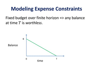
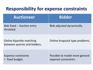
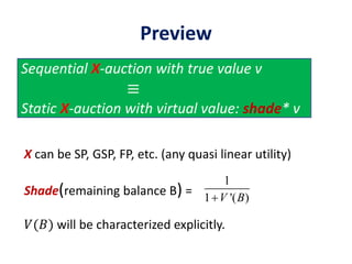
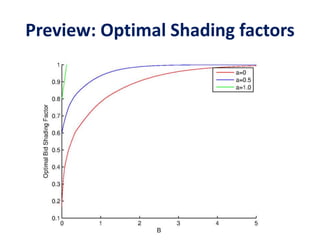
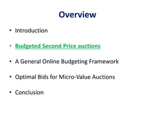
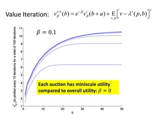
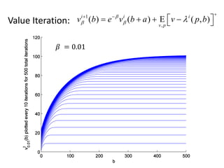
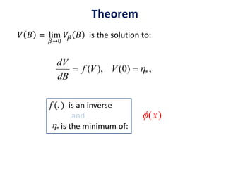
The document discusses expense-constrained bidder optimization in repeated auctions, focusing on budgeted second price auctions and online budgeting frameworks. It introduces models for optimal bid strategies under fixed income and variable auction conditions, emphasizing utility maximization while considering expense constraints. The conclusion highlights the model's applicability to online budgeting challenges and the relationship between optimal bids and virtual valuations.

1. Expense constrained bidder
optimization in repeated auctions
Ramki Gummadi
Stanford University
(Based on joint work with P. Key and A. Proutiere)

2. Overview
• Introduction/Motivation
• Budgeted Second Price Auctions
• A General Online Budgeting Framework
• Optimal Bids for Micro-Value Auctions
• Conclusion

3. Three Aspects of Sponsored Search
1. Sequential setting.
2. Micro-transactions per auction.
3. The long tail of advertisers
is expense constrained.

4. Modeling Expense Constraints
Fixed budget over finite horizon => any balance
at time 𝑇 is worthless.
Balance
time
T0
B

5. Modeling Expense Constraints
Stochastic fluctuations could cause spend rate
different from target.
Balance
time
T0
B

6. Modeling Expense Constraints
“…the nature of what this budget limit means for the
bidders themselves is somewhat of a mystery. There
seems to be some risk control element to it, some
purely administrative element to it, some bounded-
rationality element to it, and more…”
-- “Theory research at google”, SIGACT News, 2008.

7. Modeling Expense Constraints
Add a fixed income, 𝑎 per unit time to the
balance and relax time horizon.
Balance
time
0
B

8. Responsibility for expense constraints
Auctioneer Bidder
Bids fixed -- Auction entry
throttled.
Bids adjusted dynamically.
Online bipartite matching
between queries and bidders.
Online knapsack type problems.
Expense constraints
= fixed budget.
Possible to model more general
expense constraints.

9. Bid optimization

10. Preview
Sequential X-auction with true value v
≡
Static X-auction with virtual value: shade* v
X can be SP, GSP, FP, etc. (any quasi linear utility)
Shade(remaining balance B) =
𝑉(𝐵) will be characterized explicitly.
1
1 '( )V B

11. Preview: Optimal Shading factors

12. Overview
• Introduction
• Budgeted Second Price auctions
• A General Online Budgeting Framework
• Optimal Bids for Micro-Value Auctions
• Conclusion

13. Model: Budgeted Second Price
• Discrete time, indexed 𝒕 = 𝟎, 𝟏, 𝟐 …
• Balance: 𝒃(𝒕)
• Constant income per time slot - 𝒂 ≥ 𝟎
• I.I.D. environment sampled from
– Private valuation ~ 𝒗 (observable)
– Competing bid ~ 𝒑 (not observable)
• Decision variable is bid at time 𝑖: 𝒖 𝒕
– Can depend on 𝒗 𝒕 and 𝒃(𝒕), but not 𝒑(𝒕)

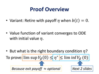
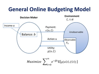
14. Model: Budgeted Second Price
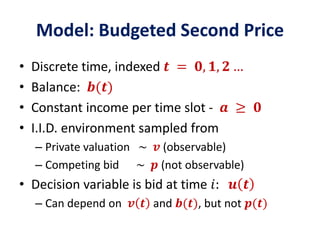
• 𝒃 𝒕 + 𝟏 = 𝒃 𝒕 + 𝒂 – 𝒑 𝒕 𝟏 𝒖 𝒕 > 𝒑 𝒕
Constraint: 𝑏 𝑡 ≥ 0 ∀ 𝑡 a.s.
• Utility: 𝒈 𝒕 = 𝒗 𝒕 − 𝒑 𝒕 𝟏 𝒖 𝒕 > 𝒑 𝒕
• Objective function: 𝒕=𝟎
∞
𝒆−𝜷𝒕
𝔼[𝒈 𝒕 ]

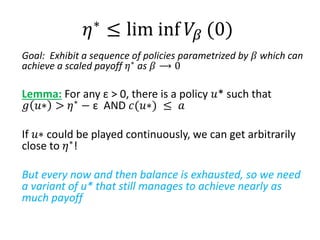
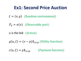
15. The Value Function
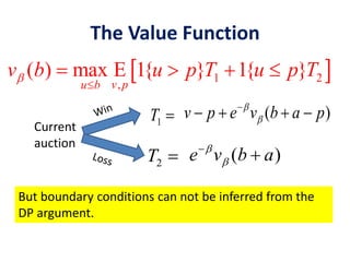
𝒗 𝜷 (𝒃) = 𝒔𝒖𝒑
𝓤 𝒕=𝟎
∞
𝒆−𝜷𝒕
𝔼[𝒈 𝒕 ] | 𝒃 𝟎 = 𝒃
• 𝑣 𝛽 (𝑏) : max utility starting with balance 𝑏
• Can use dynamic programming (“one step look
ahead”) to write out a functional fixed point
relation.

16. The Value Function
 1 2
,
( ) max E 1{ } 1{ }
v pu b
v b u p T u p T

   
( )v p e v b a p


   
( )e v b a



But boundary conditions can not be inferred from the
DP argument.
Current
auction
1T 
2T 

17. Future opportunity cost
Characterization of value function
“Effective price” for nominal 𝒑 at balance 𝒃:
Theorem: Optimal bid is 𝒖*:
i.e: Buy all auctions with “effective price” ≤ 𝑣
𝑣 𝛽(𝑏) is a functional fixed point to:
( , )*u b v 
 ,
( ) ( ) ( , )
v p
v b e v b a v p b
  

    
( , ) ( ( ) ( ))p b p e v b a v b a p
  
     

18. 1
,
( ) ( ) ( , )i i i
v p
v b e v b a v p b
  
 
      Value Iteration:
𝛽 = 0.1
Each auction has miniscule utility
compared to overall utility: 𝛽 ≈ 0

19. Value Iteration:
𝛽 = 0.01
1
,
( ) ( ) ( , )i i i
v p
v b e v b a v p b
  
 
      

20. Numerical estimation when 𝛽 is small:
• State space quantization errors propagate due
to lack of boundary value.
• Need longer iterations over larger state space.
𝛽 ⟶ 0 will be studied under scaling:
( ) ( ) ( / )V B v b v B    
Limiting case: micro-value auctions

21. Overview
• Introduction
• Budgeted Second Price Auctions
• A General Online Budgeting Framework
• Optimal Bids for Micro-Value Auctions
• Conclusion

22. General Online Budgeting Model
Decision Maker
Environment
𝜉, i.i.d
Unobservable
Observable
ℱ0
Balance: 𝑏
Utility:
𝑔(𝑢, 𝜉)
Action 𝑢
Payment:
𝑐(𝑢, 𝜉)
Income 𝑎
𝑀𝑎𝑥𝑖𝑚𝑖𝑧𝑒
𝑡=0
∞
𝑒−𝛽𝑡 𝔼 𝑔(𝑢 𝑡 , 𝜉 𝑡 )

23. Ex1: Second Price Auction
𝜉 = 𝑣, 𝑝 (Random environment)
ℱ0 = 𝜎 𝑣 (Observable part)
𝑢 is the bid (Action)
𝑔 𝑢, 𝜉 = (𝑣 − 𝑝)𝟏 𝑢>𝑝 (Utility function)
𝑐 𝑢, 𝜉 = 𝑝𝟏 𝑢>𝑝 (Payment function)

24. Ex2: GSP Auction
Random environment:
𝜉 = 𝑣, 𝑝1 , … , 𝑝L , 𝛾1, … , 𝛾 𝐿
Observable part: ℱ0 = 𝜎 𝑣
Action: 𝑢 is the bid
Utility function:
Payment function:
1
1
( , ) 1{ } ( )
L
l l l l
l
g u p u p v p 

   
1
1
( , ) 1{ }
L
l l l l
l
c u p u p p 

  
Click events for L slots

25. Overview
• Introduction
• Budgeted Second Price Auctions
• A General Online Budgeting Framework
• Optimal Bids for Micro-Value Auctions
• Conclusion

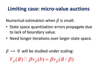
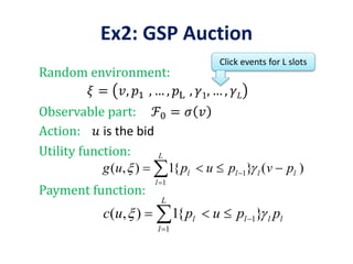
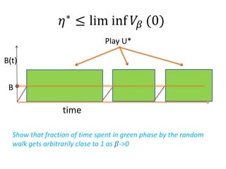
26. Limiting Regime: 𝛽 ⟶ 0
( ) ( ) ( / )V B v b v B    
Notation:
(( ]) [ , )E g ug u 
(( ]) [ , )E c uc u 

27. 𝑓(. ) is an inverse
and
is the minimum of:
Theorem
*( ), (0) ,
dV
f V V
dB
 
( )x
𝑉 𝐵 = lim
𝛽→0
𝑉𝛽 𝐵 is the solution to:
*

28. *( ') , (0) ,V V V  
0
( ) sup( ( ) ( ) )
u
x ax g u c u x

 
F
* 0min ( )x x 
𝑥
𝑉
𝑉’ 𝐵
𝑉(𝐵)
Theorem
( )x
*

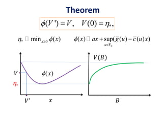
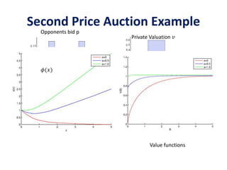
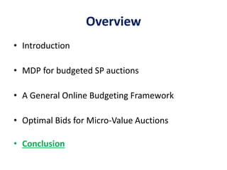
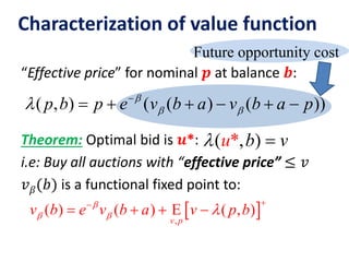
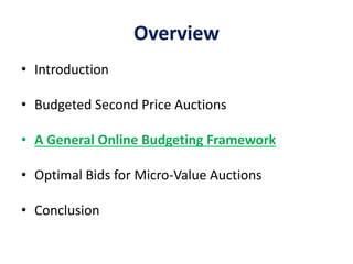
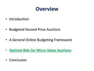
29. 𝜙 𝑥 = 𝑎𝑥 + sup
𝑢∈ℱ0
( 𝑔(𝑢) − 𝑐(𝑢)𝑥)
= 𝑎 𝑥 + sup
𝑢∈𝜎(𝑣)
𝔼 𝟏 𝑢>𝑝(𝑣 − 𝑝 1 + 𝑥 )
= 𝑎 𝑥 + 𝔼 (𝑣 − 𝑝 1 + 𝑥) +
Application to Second Price Auctions
𝐸[𝟏 𝑢>𝑝 𝑣 − 𝑝 ]
𝐸[𝟏 𝑢>𝑝p]

30. Second Price Auction Example
Opponents bid p
Private Valuation 𝑣
𝜙(𝑥)
Value functions

31. Optimal bid
 
0 ( )
( )
sup( ( ) ( ) '( )) sup 1{ }( (1 '( ))
sup 1{ }
1 '( )
u u v
u v
g u c u V B uE p v p V B
v
u p p
V
E
B


 

    
 
    
 
 
 
F
i.e., Static SP with shaded valuation:
1 '( )
v
V B
𝒖* at balance B solves:

32. Optimal Scaling factor

33. Optimal Bid: GSP
0
1
( ) 1
sup( ( ) ( ) '( ))
sup 1{ }
1 '( )
u
L
l l l l
u v l
g u c u V B
v
p u p p
V
E
B



 

 
   
 
 
  

F
Static GSP with “virtual valuation”:
1 '( )
v
V B

34. Proof Overview
• Variant: Retire with payoff 𝜂 when 𝑏 𝑡 = 0.
• Value function of variant converges to ODE
with initial value 𝜂.
• But what is the right boundary condition 𝜂?
To prove: lim sup 𝑉𝛽 0 ≤ 𝜂∗
≤ lim inf 𝑉𝛽 (0)
Because exit payoff ≈ optional Next 2 slides

35. Goal: Exhibit a sequence of policies parametrized by 𝛽 which can
achieve a scaled payoff 𝜂∗
as 𝛽 ⟶ 0
Lemma: For any ε > 0, there is a policy 𝑢* such that
𝑔 𝑢∗ > 𝜂∗
− ε AND 𝑐(𝑢∗) ≤ 𝑎
If 𝑢∗ could be played continuously, we can get arbitrarily
close to 𝜂∗
!
But every now and then balance is exhausted, so we need
a variant of u* that still manages to achieve nearly as
much payoff
𝜂∗ ≤ lim inf 𝑉𝛽 (0)

36. time
B(t)
B
Play U*
𝜂∗ ≤ lim inf 𝑉𝛽 (0)
Show that fraction of time spent in green phase by the random
walk gets arbitrarily close to 1 as 𝛽->0

37. Overview
• Introduction
• MDP for budgeted SP auctions
• A General Online Budgeting Framework
• Optimal Bids for Micro-Value Auctions
• Conclusion

38. Conclusion
• A two parameter model for expense
constraints in online budgeting problems.
• Optimal bid can be mapped to static auction
with a shaded virtual valuation.
• Paper has more contents: MFE analysis and a
finite horizon model.