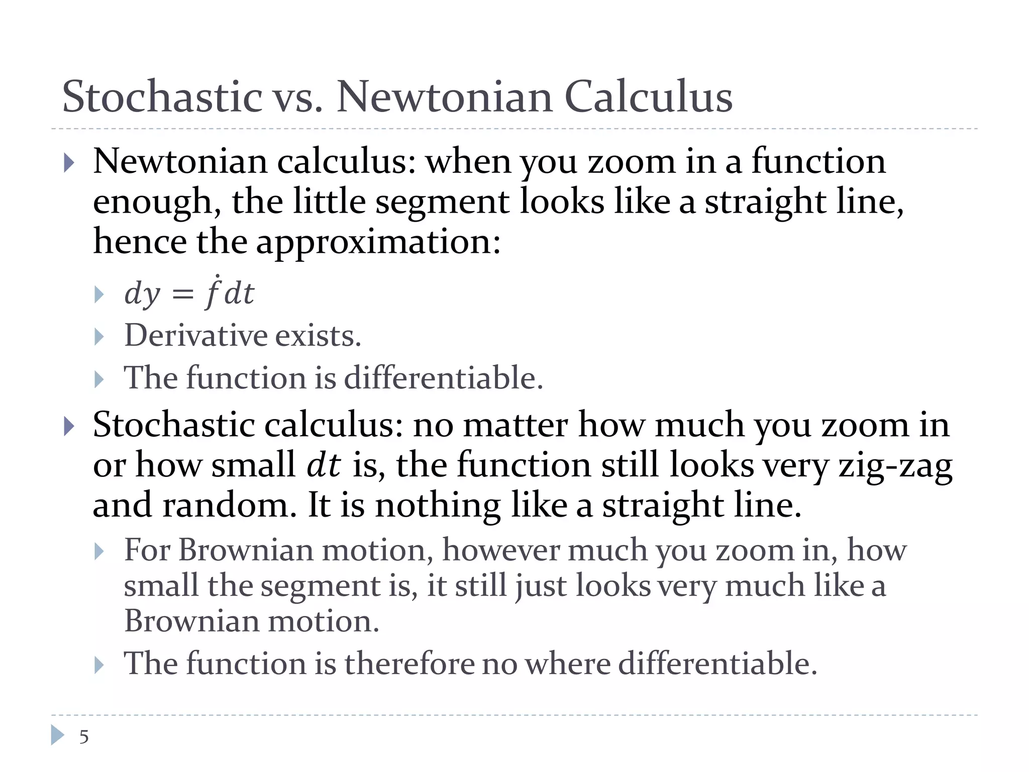
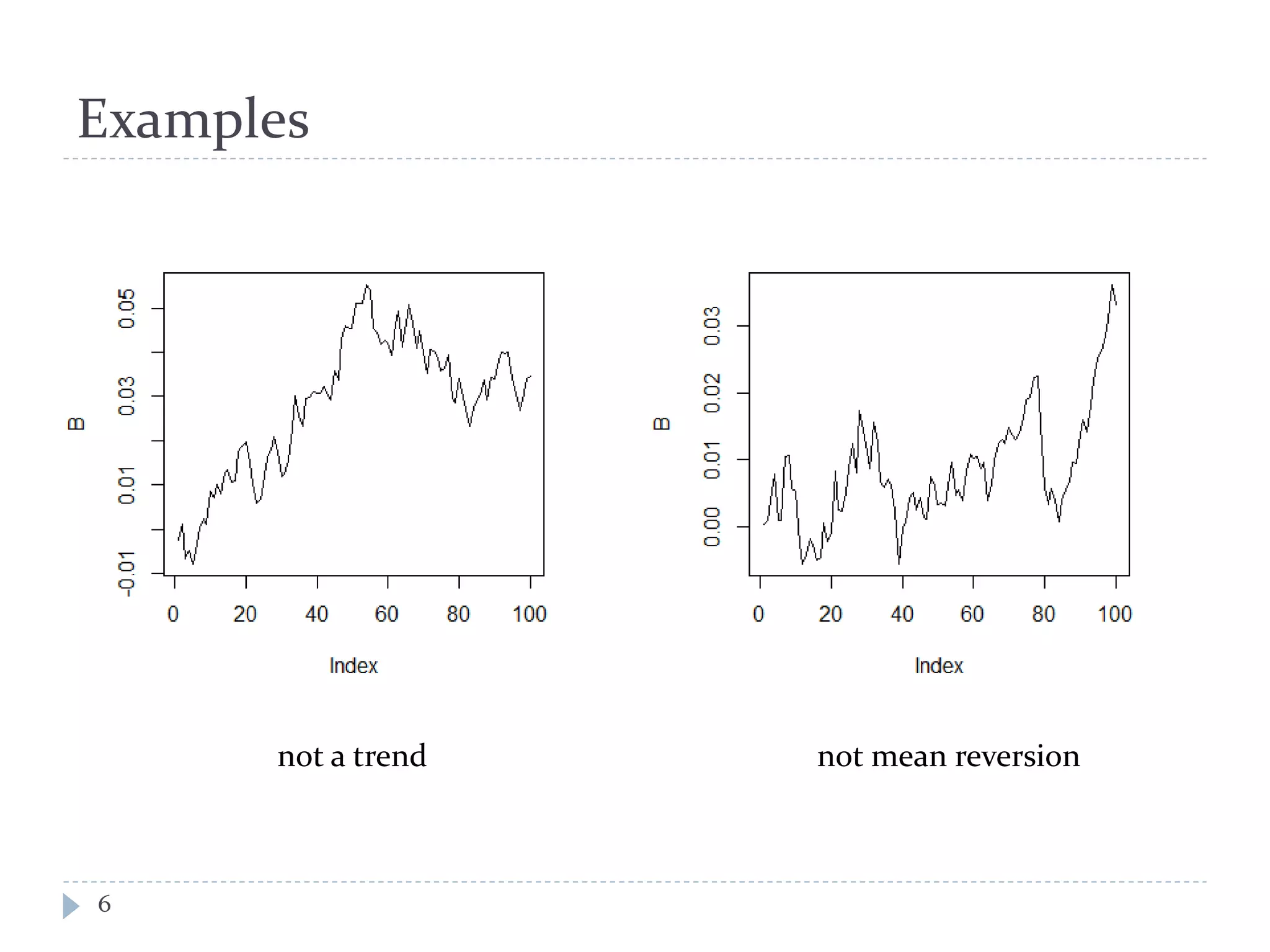
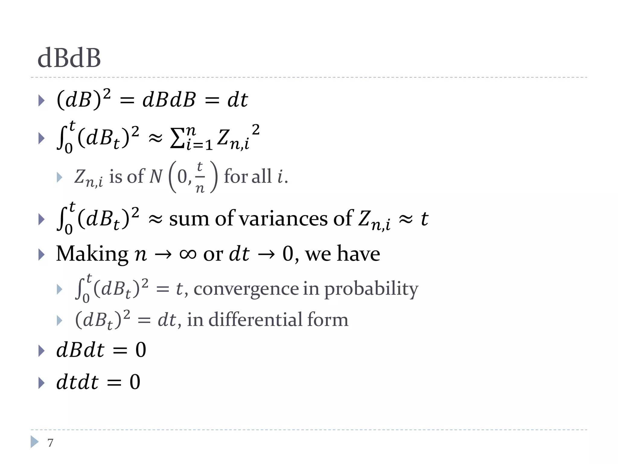
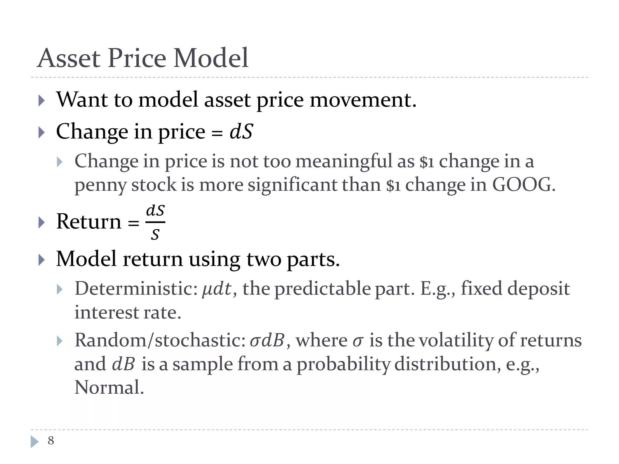
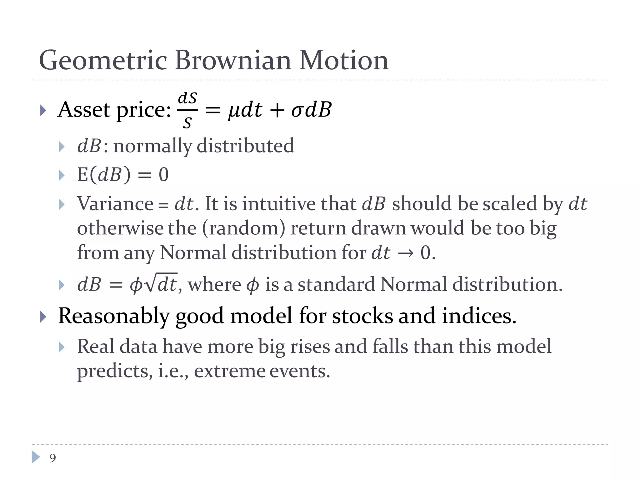
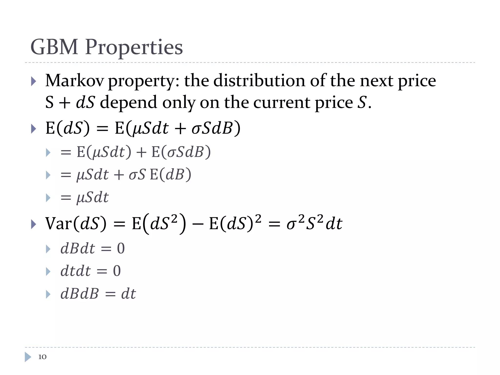
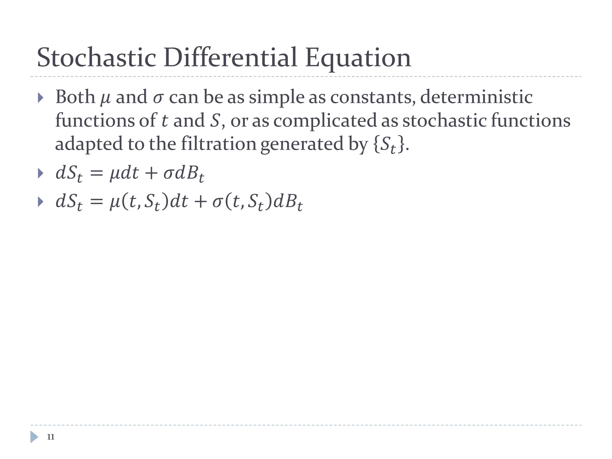
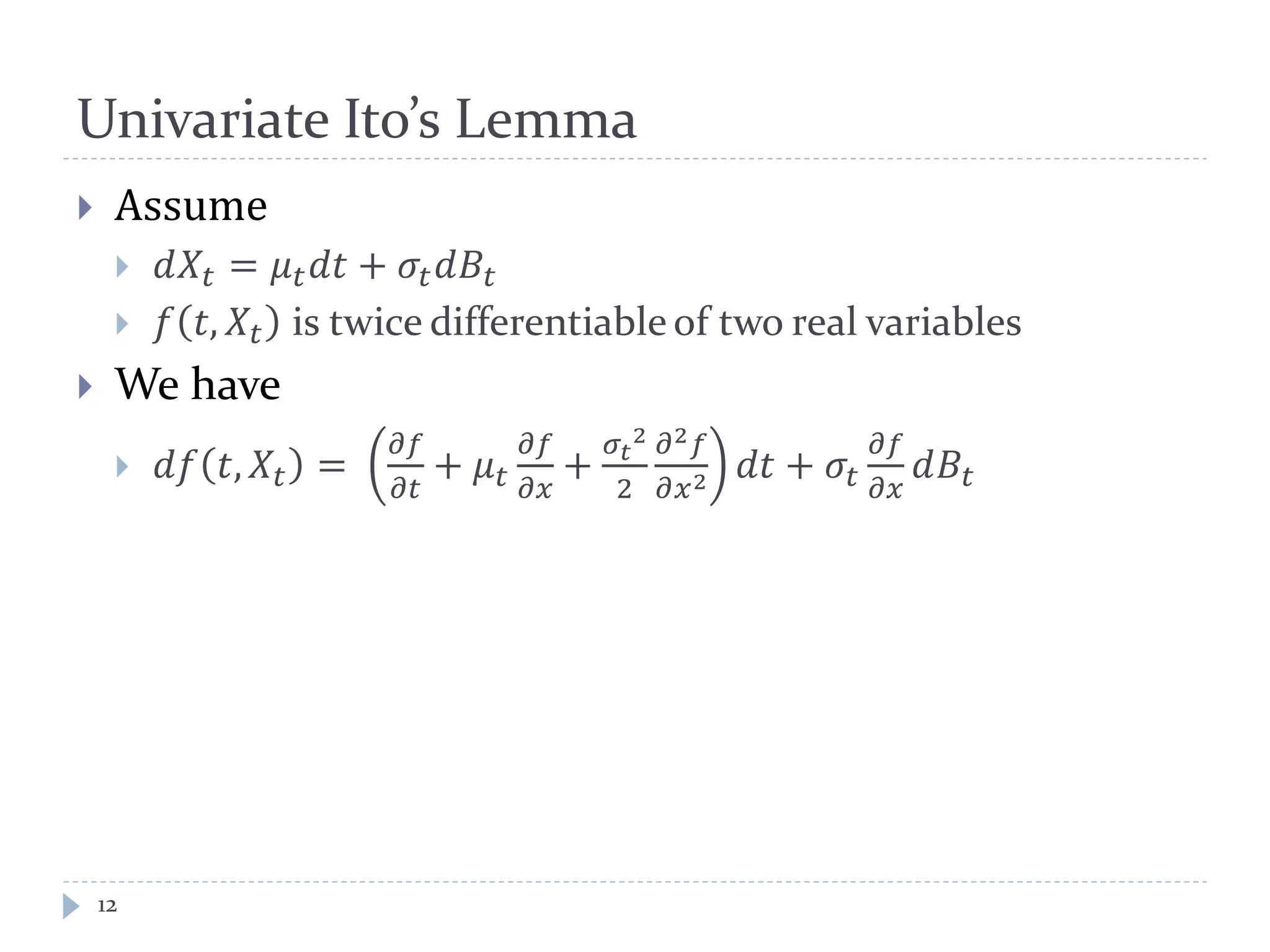
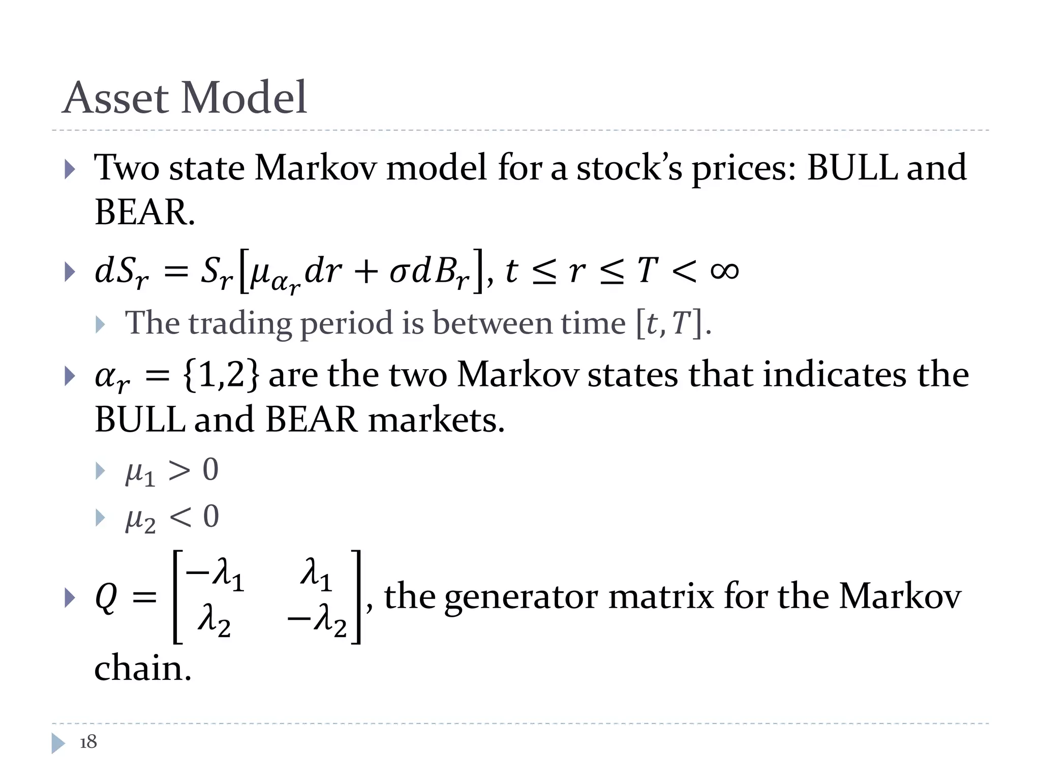
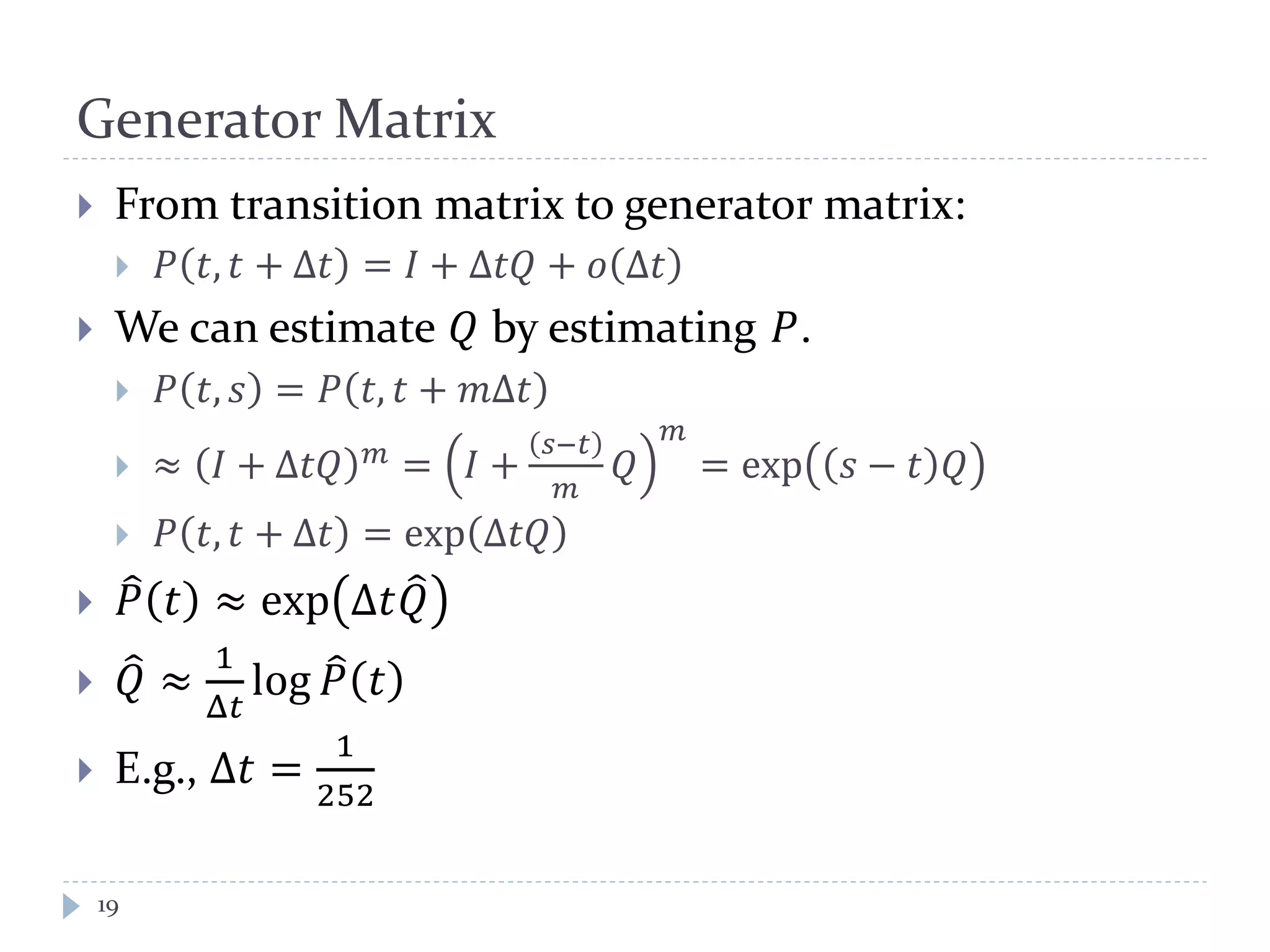
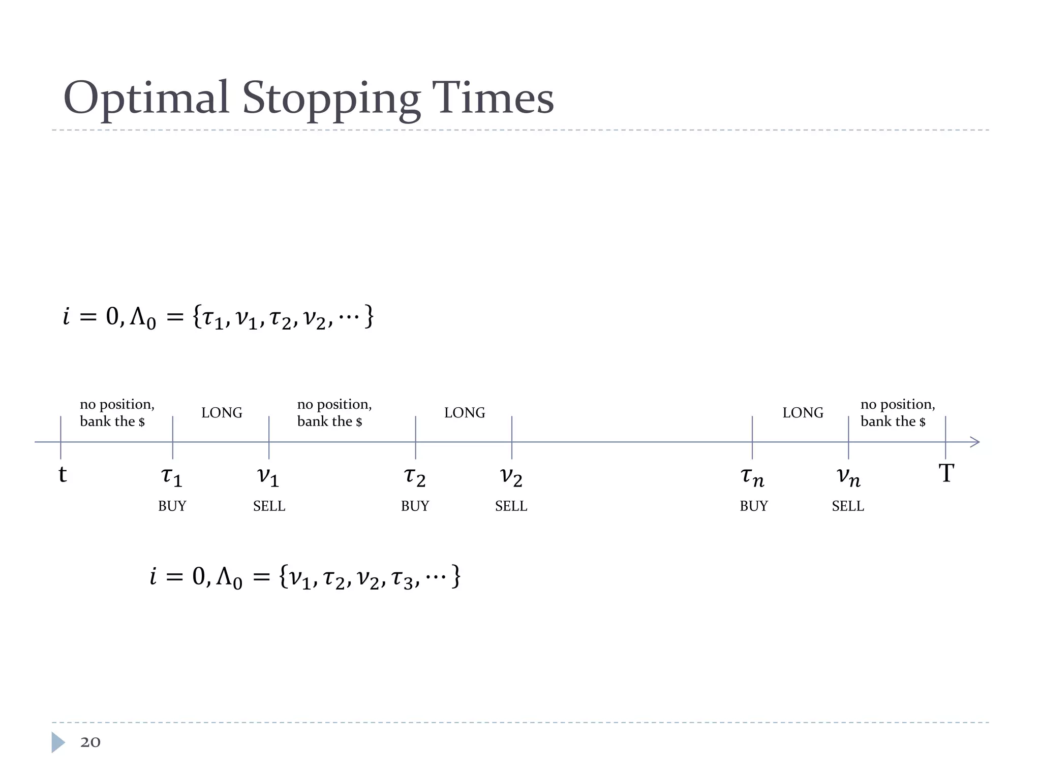
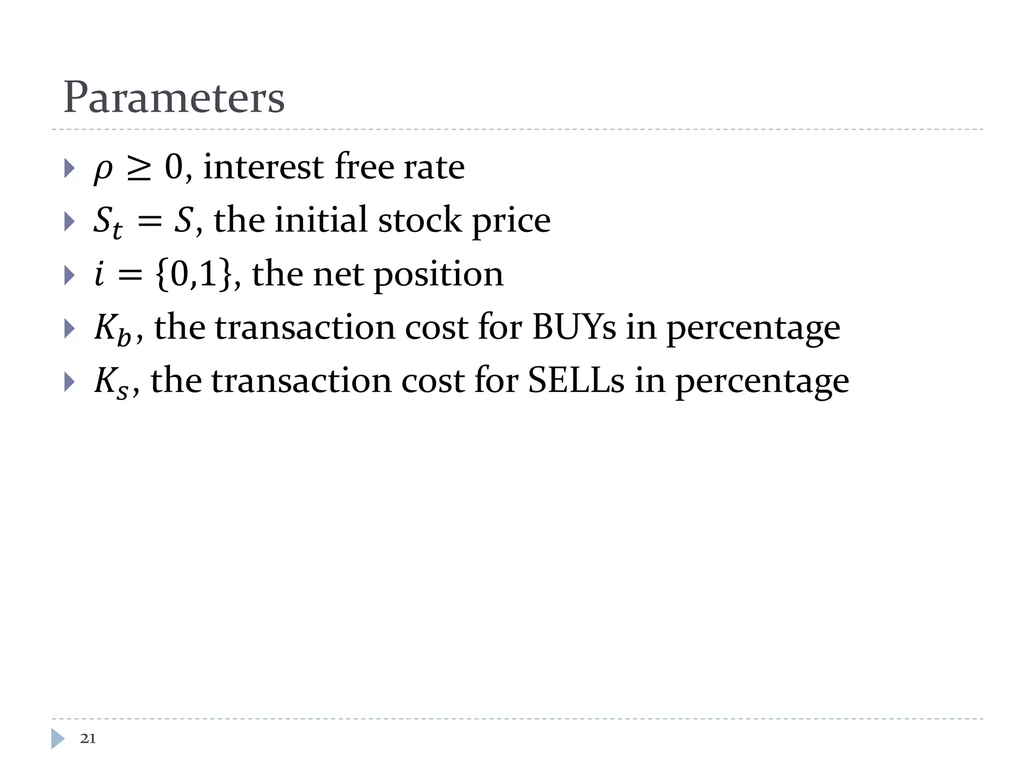
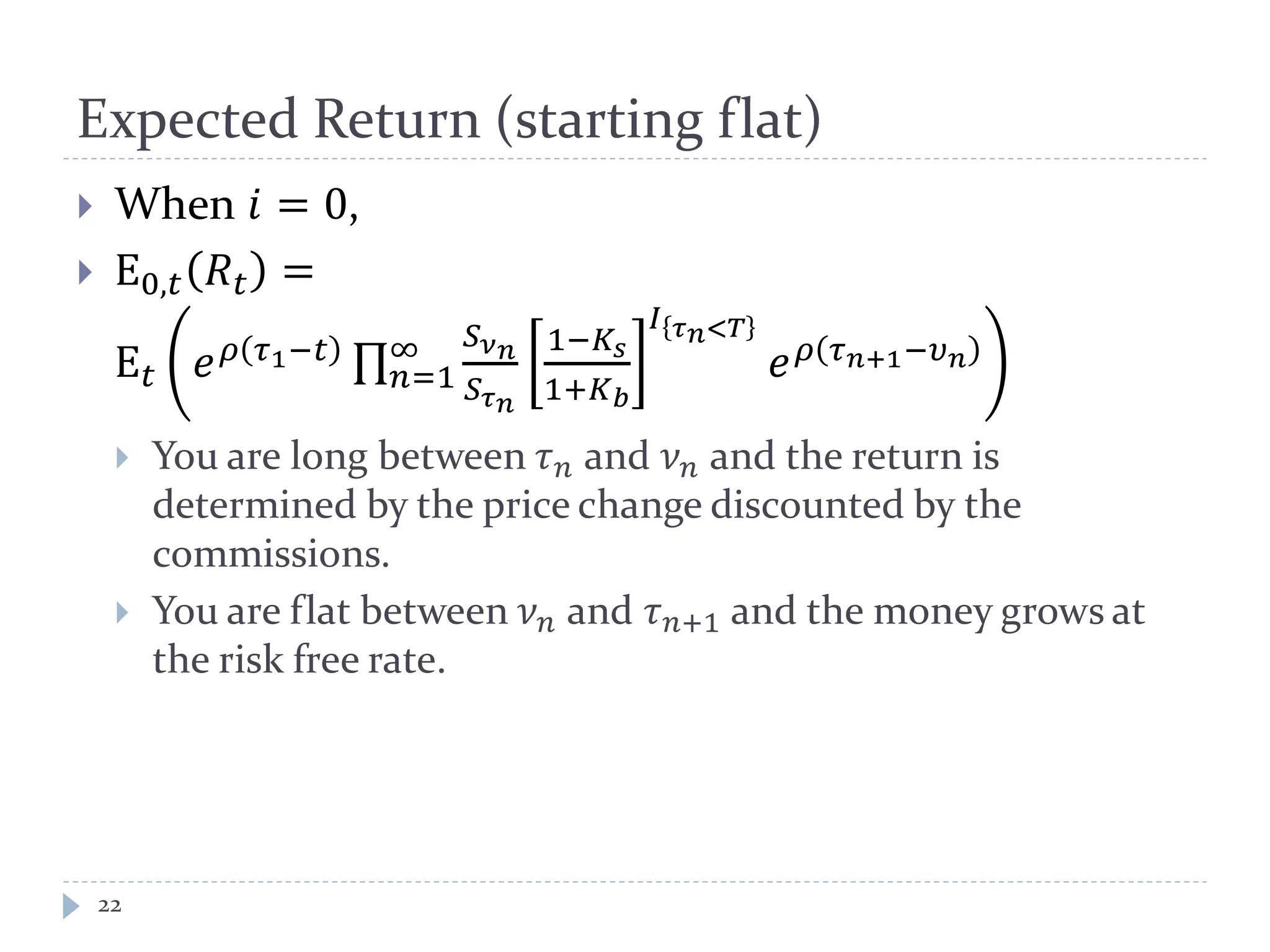
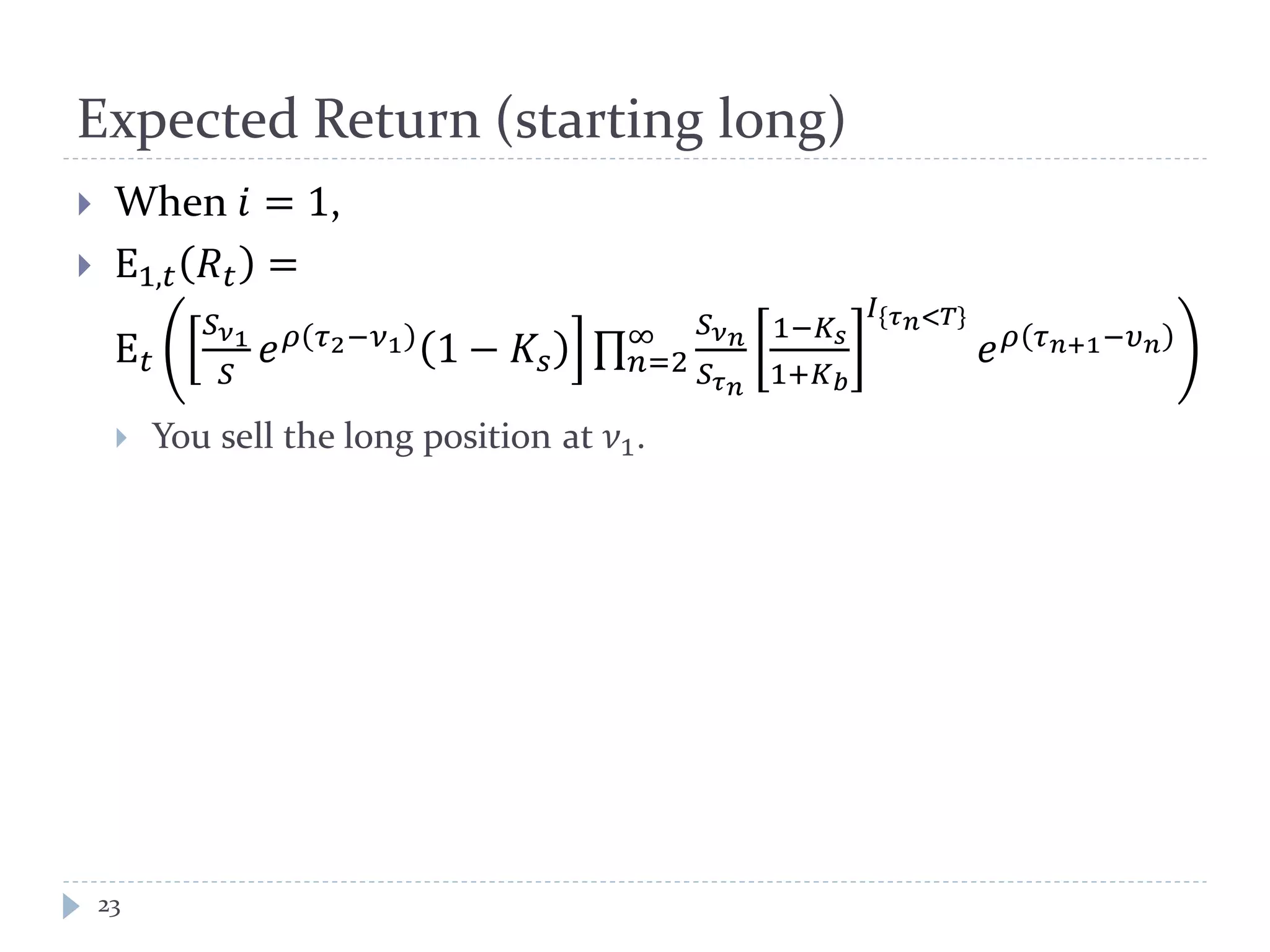
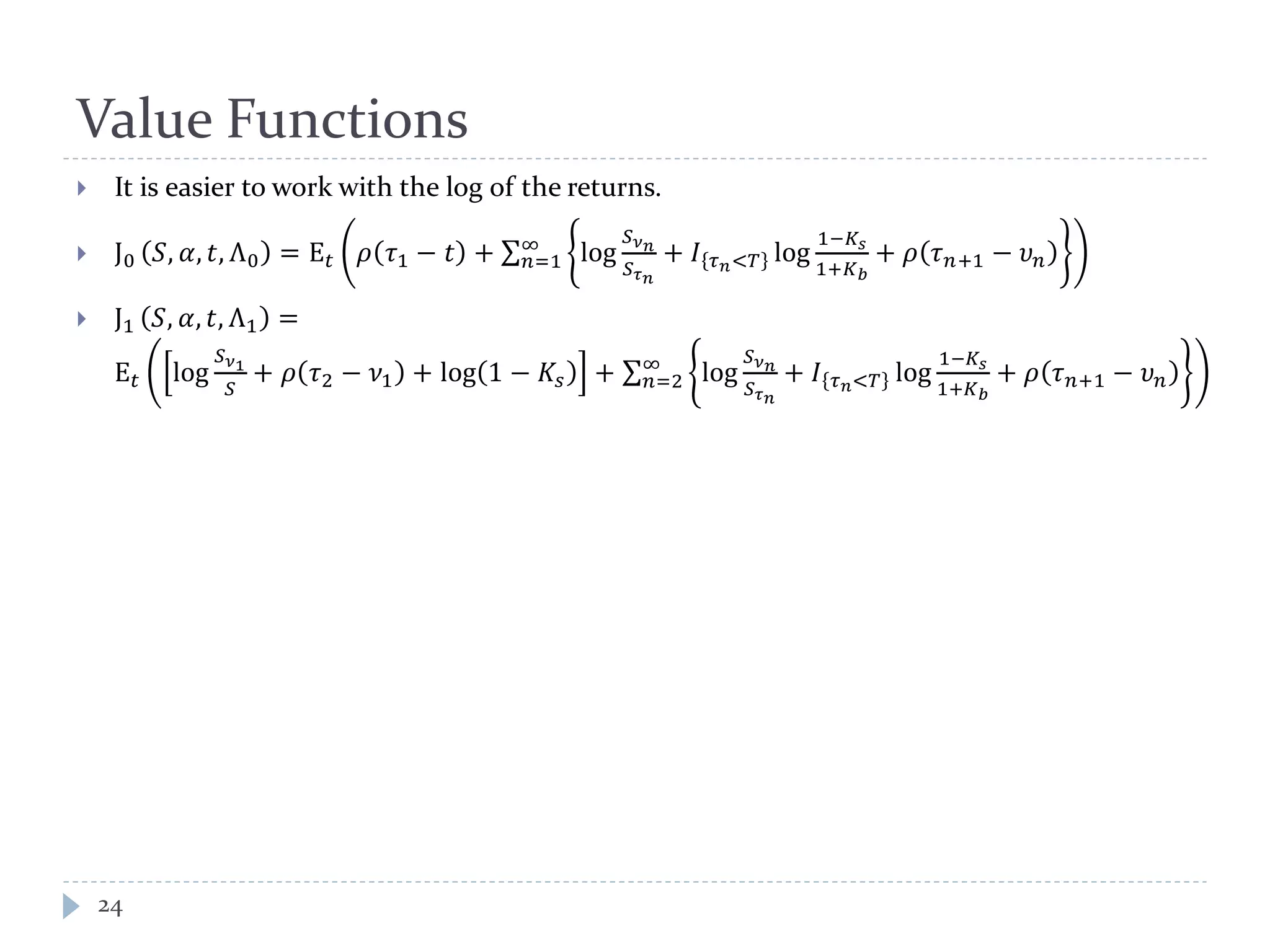
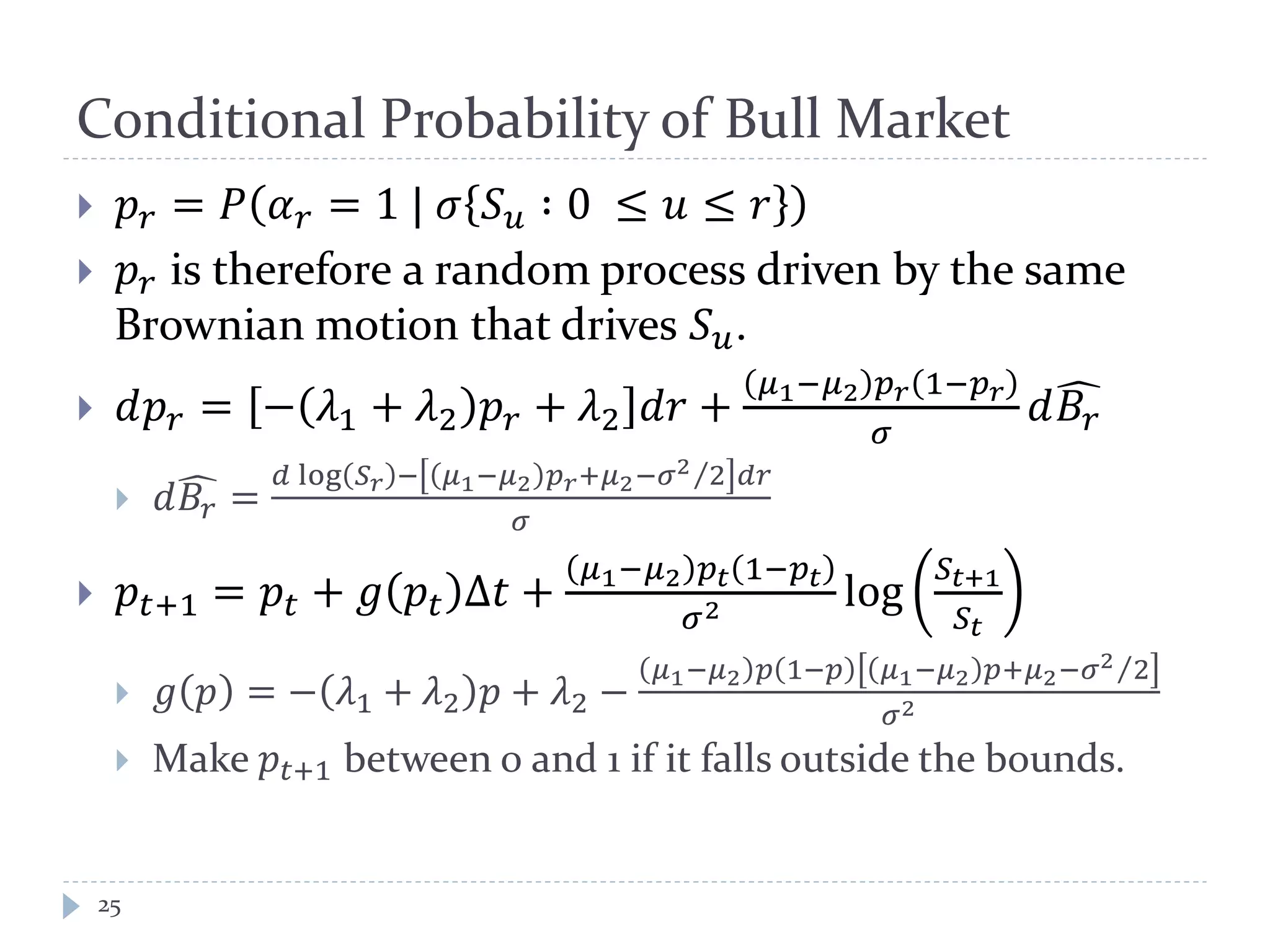
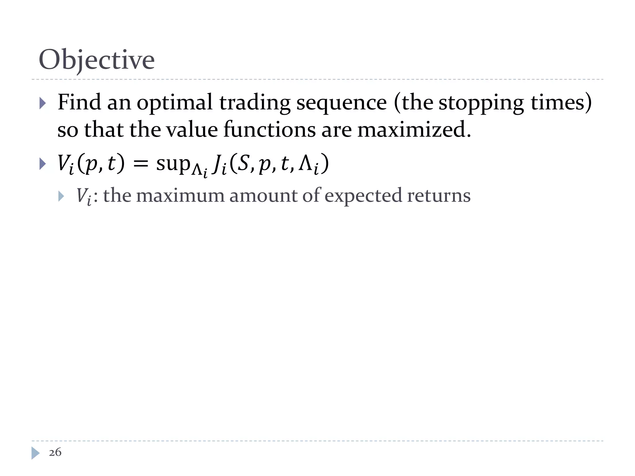
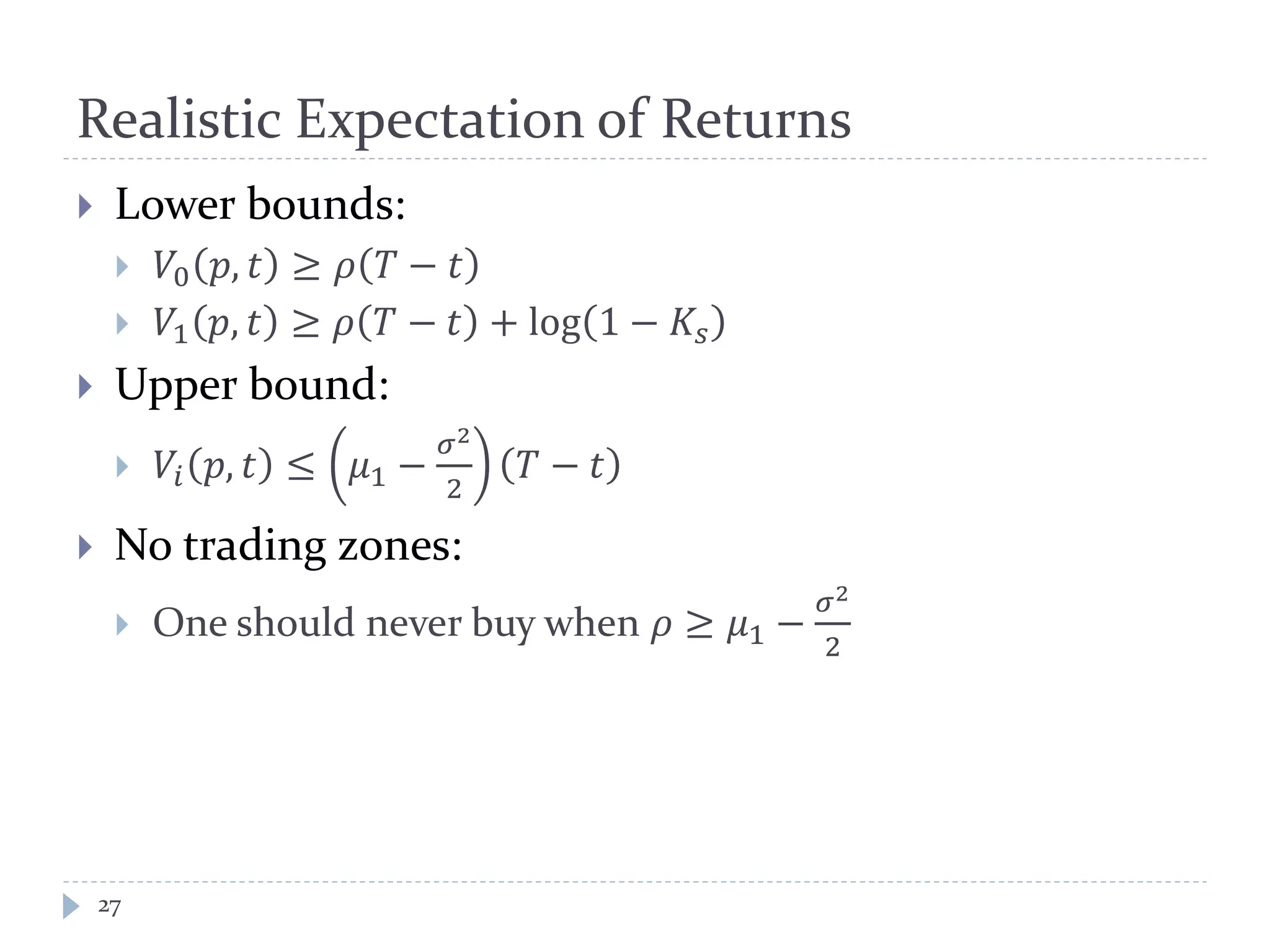
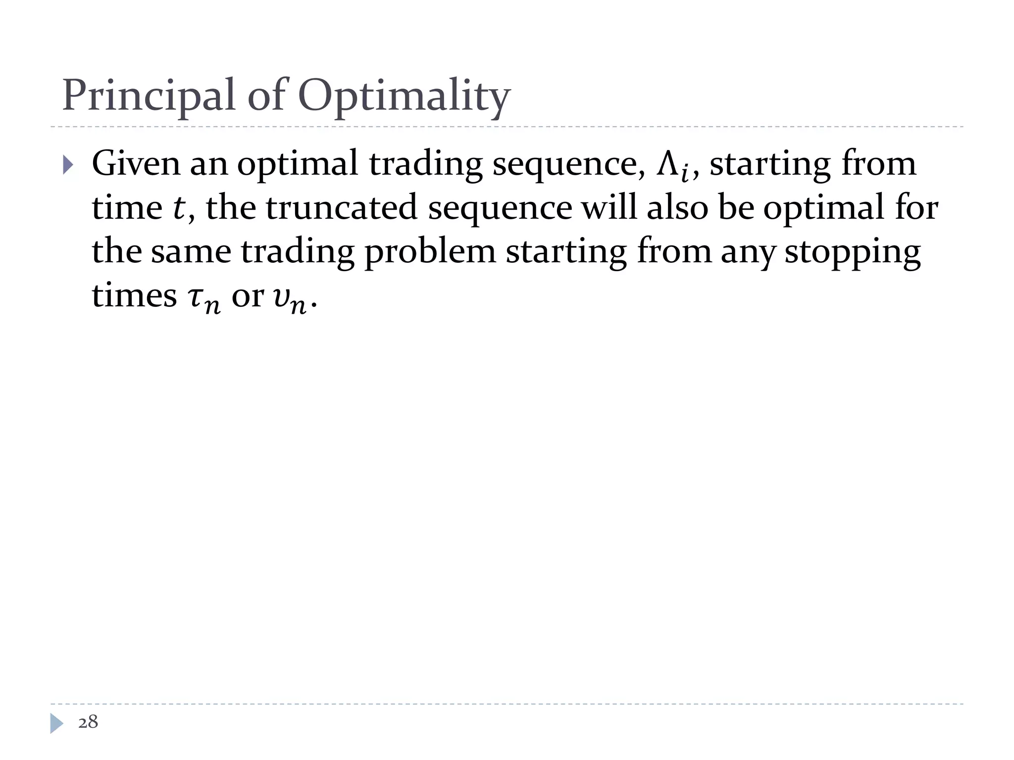
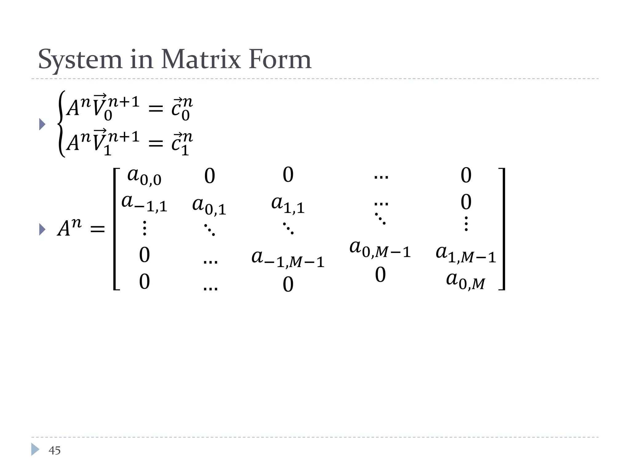
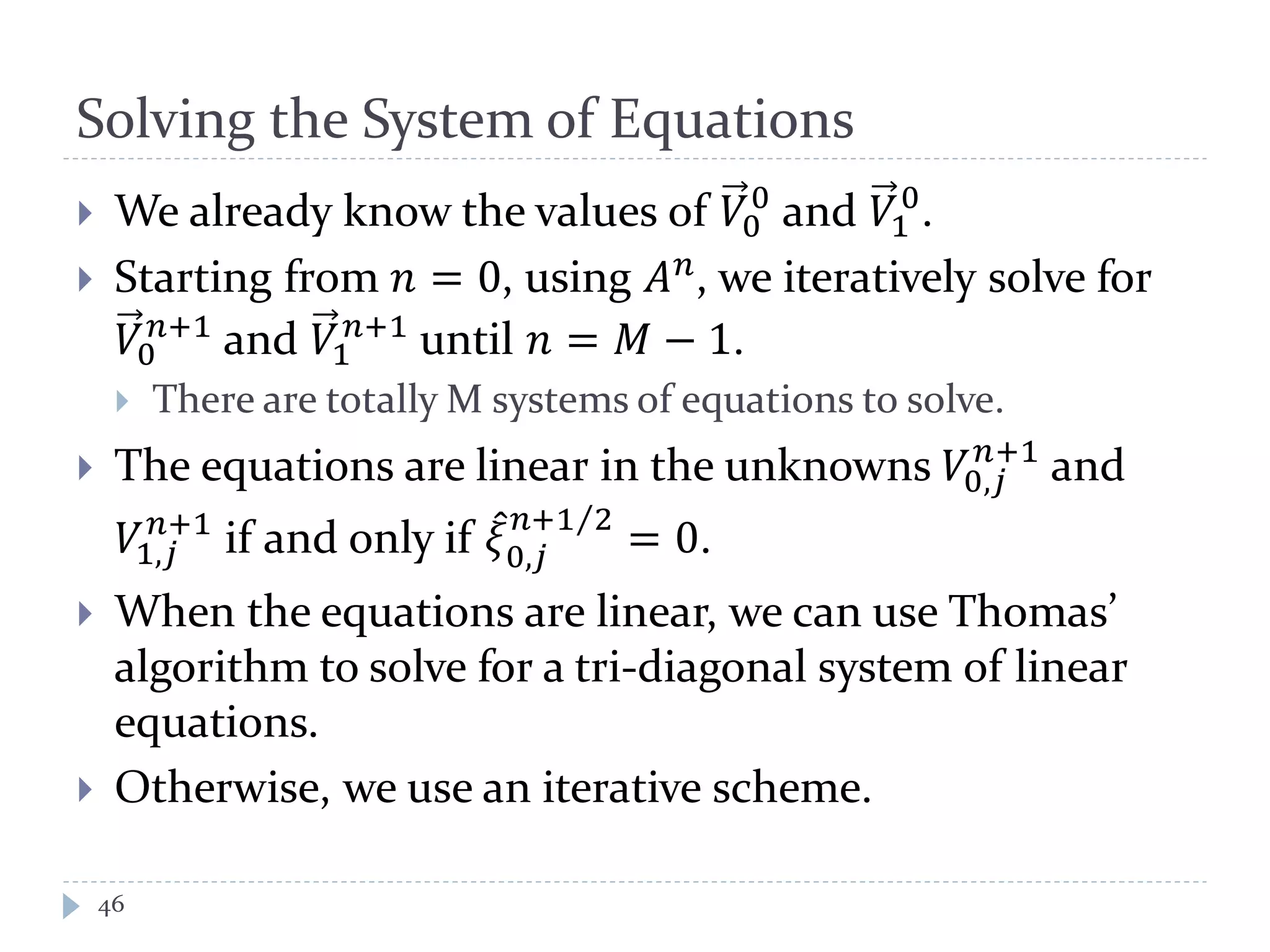
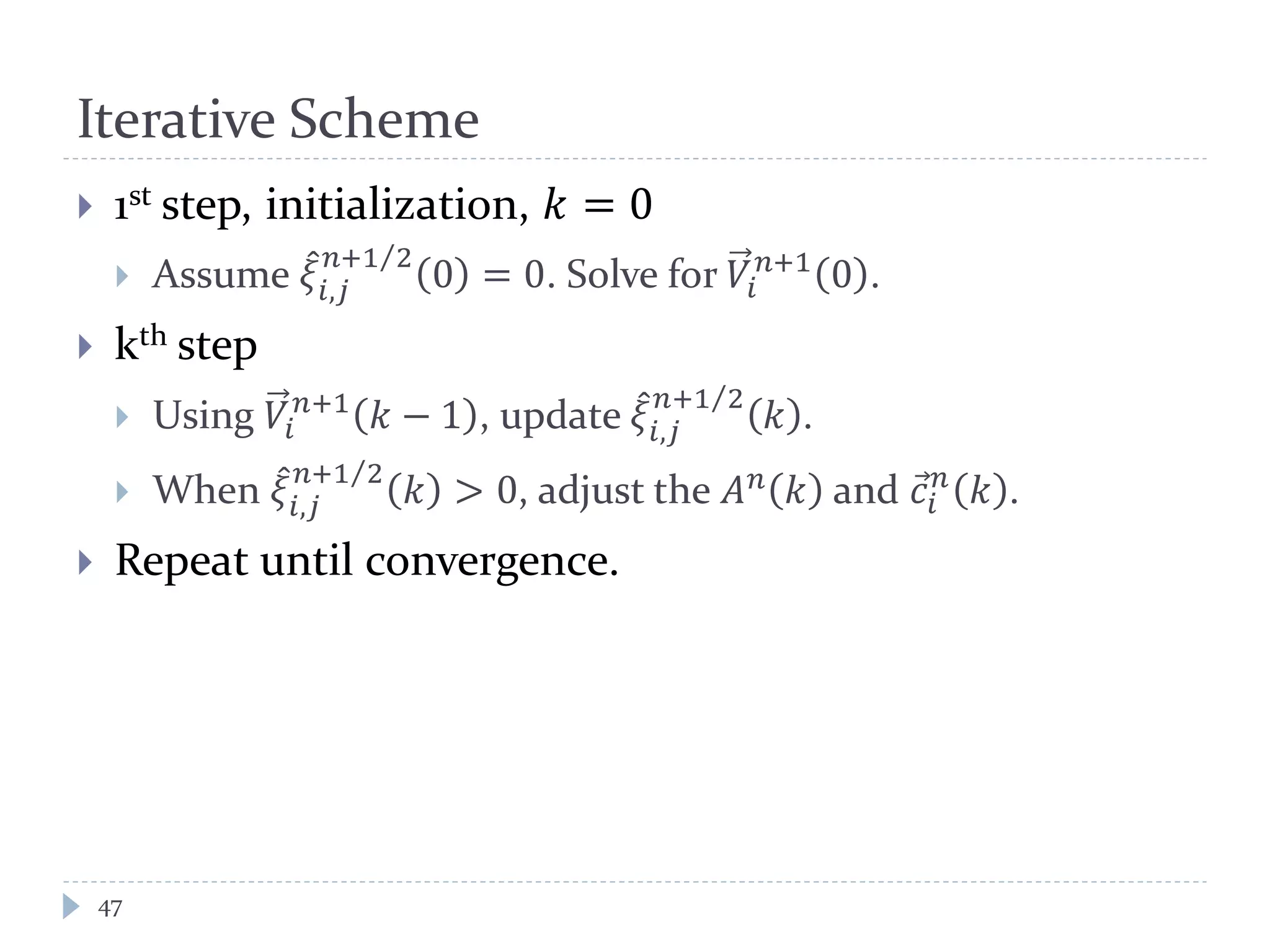
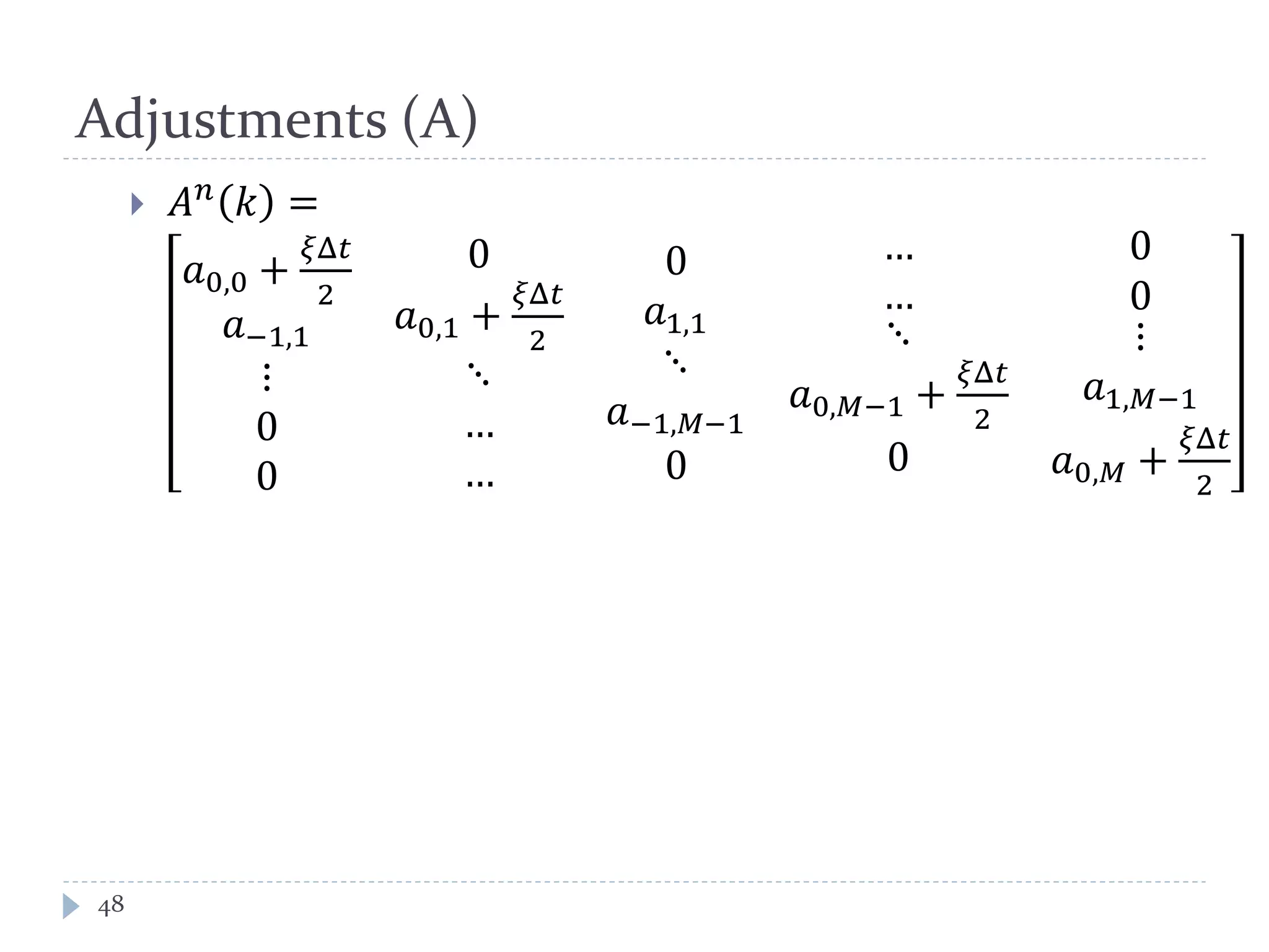
SlideShare a Scribd company logo
1 of 52
Download to read offline
Introduction to Algorithmic Trading Strategies
Lecture 3
Trend Following
Haksun Li
haksun.li@numericalmethod.com
www.numericalmethod.com
References
2
๏ฝ Introduction to Stochastic Calculus with Applications.
Fima C Klebaner. 2nd Edition.
๏ฝ Estimating continuous time transition matrices from
discretely observed data. Inamura, Yasunari. April
2006.
๏ฝ Optimal Trend Following Trading Rules. Dai, Min and
Zhang, Qing and Zhu, Qiji Jim. 2011.
Stochastic Calculus
3
Brownian Motion
4
๏ฝ Independence of increments.
๏ฝ ๐‘‘๐‘‘ = ๐ต ๐‘ก โˆ’ ๐ต ๐‘  is independent of any history up to ๐‘ .
๏ฝ Normality of increments.
๏ฝ ๐‘‘๐‘‘ is normally distributed with mean 0 and variance ๐‘ก โˆ’ ๐‘ .
๏ฝ Continuity of paths.
๏ฝ ๐ต ๐‘ก is a continuous function of ๐‘ก.
Stochastic vs. Newtonian Calculus
5
๏ฝ Newtonian calculus: when you zoom in a function
enough, the little segment looks like a straight line,
hence the approximation:
๏ฝ ๐‘‘๐‘‘ = ๐‘“ฬ‡ ๐‘‘๐‘‘
๏ฝ Derivative exists.
๏ฝ The function is differentiable.
๏ฝ Stochastic calculus: no matter how much you zoom in
or how small ๐‘‘๐‘‘ is, the function still looks very zig-zag
and random. It is nothing like a straight line.
๏ฝ For Brownian motion, however much you zoom in, how
small the segment is, it still just looks very much like a
Brownian motion.
๏ฝ The function is therefore no where differentiable.
Examples
6
not a trend not mean reversion
dBdB
7
๏ฝ ๐‘‘๐‘‘ 2 = ๐‘‘๐‘‘๐‘‘๐‘‘ = ๐‘‘๐‘‘
๏ฝ โˆซ ๐‘‘๐ต๐‘ก
2๐‘ก
0
โ‰ˆ โˆ‘ ๐‘ ๐‘›,๐‘–
2๐‘›
๐‘–=1
๏ฝ ๐‘ ๐‘›,๐‘– is of ๐‘ 0,
๐‘ก
๐‘›
for all ๐‘–.
๏ฝ โˆซ ๐‘‘๐ต๐‘ก
2๐‘ก
0
โ‰ˆ sum of variances of ๐‘ ๐‘›,๐‘– โ‰ˆ ๐‘ก
๏ฝ Making ๐‘› โ†’ โˆž or ๐‘‘๐‘‘ โ†’ 0, we have
๏ฝ โˆซ ๐‘‘๐ต๐‘ก
2๐‘ก
0
= ๐‘ก, convergence in probability
๏ฝ ๐‘‘๐ต๐‘ก
2 = ๐‘‘๐‘‘, in differential form
๏ฝ ๐‘‘๐‘‘๐‘‘๐‘ก = 0
๏ฝ ๐‘‘๐‘ก๐‘‘๐‘‘ = 0
Asset Price Model
8
๏ฝ Want to model asset price movement.
๏ฝ Change in price = ๐‘‘๐‘‘
๏ฝ Change in price is not too meaningful as $1 change in a
penny stock is more significant than $1 change in GOOG.
๏ฝ Return =
๐‘‘๐‘‘
๐‘†
๏ฝ Model return using two parts.
๏ฝ Deterministic: ๐œ‡๐‘‘๐‘‘, the predictable part. E.g., fixed deposit
interest rate.
๏ฝ Random/stochastic: ๐œŽ๐‘‘๐‘‘, where ๐œŽ is the volatility of returns
and ๐‘‘๐ต is a sample from a probability distribution, e.g.,
Normal.
Geometric Brownian Motion
9
๏ฝ Asset price:
๐‘‘๐‘‘
๐‘†
= ๐œ‡๐œ‡๐œ‡ + ๐œŽ๐œŽ๐ต
๏ฝ ๐‘‘๐ต: normally distributed
๏ฝ E ๐‘‘๐ต = 0
๏ฝ Variance = ๐‘‘๐‘‘. It is intuitive that ๐‘‘๐ต should be scaled by ๐‘‘๐‘‘
otherwise the (random) return drawn would be too big
from any Normal distribution for ๐‘‘๐‘‘ โ†’ 0.
๏ฝ ๐‘‘๐ต = ๐œ™ ๐‘‘๐‘‘, where ๐œ™ is a standard Normal distribution.
๏ฝ Reasonably good model for stocks and indices.
๏ฝ Real data have more big rises and falls than this model
predicts, i.e., extreme events.
GBM Properties
10
๏ฝ Markov property: the distribution of the next price
S + ๐‘‘๐‘‘ depend only on the current price ๐‘†.
๏ฝ E ๐‘‘๐‘† = E ๐œ‡๐‘†๐‘‘๐‘‘ + ๐œŽ๐‘†๐‘‘๐ต
๏ฝ = E ๐œ‡๐œ‡๐œ‡๐œ‡ + E ๐œŽ๐œŽ๐œŽ๐ต
๏ฝ = ๐œ‡๐œ‡๐œ‡๐œ‡ + ๐œŽ๐œŽ E ๐‘‘๐ต
๏ฝ = ๐œ‡๐œ‡๐œ‡๐œ‡
๏ฝ Var ๐‘‘๐‘‘ = E ๐‘‘๐‘‘2 โˆ’ E ๐‘‘๐‘‘ 2 = ๐œŽ2 ๐‘†2 ๐‘‘๐‘‘
๏ฝ ๐‘‘๐ต๐‘‘๐‘‘ = 0
๏ฝ ๐‘‘๐‘‘๐‘‘๐‘‘ = 0
๏ฝ ๐‘‘๐ต๐‘‘๐ต = ๐‘‘๐‘‘
Stochastic Differential Equation
11
๏ฝ Both ๐œ‡ and ๐œŽ can be as simple as constants, deterministic
functions of ๐‘ก and ๐‘†, or as complicated as stochastic functions
adapted to the filtration generated by ๐‘†๐‘ก .
๏ฝ ๐‘‘๐‘†๐‘ก = ๐œ‡๐œ‡๐œ‡ + ๐œŽ๐œŽ๐ต๐‘ก
๏ฝ ๐‘‘๐‘†๐‘ก = ๐œ‡ ๐‘ก, ๐‘†๐‘ก ๐‘‘๐‘‘ + ๐œŽ ๐‘ก, ๐‘†๐‘ก ๐‘‘๐ต๐‘ก
Univariate Itoโ€™s Lemma
12
๏ฝ Assume
๏ฝ ๐‘‘๐‘‹๐‘ก = ๐œ‡ ๐‘ก ๐‘‘๐‘‘ + ๐œŽ๐‘ก ๐‘‘๐ต๐‘ก
๏ฝ ๐‘“ ๐‘ก, ๐‘‹๐‘ก is twice differentiable of two real variables
๏ฝ We have
๏ฝ ๐‘‘๐‘‘ ๐‘ก, ๐‘‹๐‘ก =
๐œ•๐œ•
๐œ•๐œ•
+ ๐œ‡ ๐‘ก
๐œ•๐œ•
๐œ•๐œ•
+
๐œŽ๐‘ก
2
2
๐œ•2 ๐‘“
๐œ•๐‘ฅ2 ๐‘‘๐‘‘ + ๐œŽ๐‘ก
๐œ•๐œ•
๐œ•๐œ•
๐‘‘๐ต๐‘ก
โ€œProofโ€
13
๏ฝ Taylor series
๏ฝ ๐‘‘๐‘“ ๐‘ก, ๐‘‹
๏ฝ = ๐‘“๐‘ก ๐‘‘๐‘‘ + ๐‘“๐‘‹ ๐‘‘๐‘‹ +
1
2
๐‘“๐‘ก๐‘ก ๐‘‘๐‘‘๐‘‘๐‘‘ + ๐‘“๐‘ก๐‘‹ ๐‘‘๐‘‘๐‘‘๐‘‹ + ๐‘“๐‘‹๐‘‹ ๐‘‘๐‘‹๐‘‘๐‘ก + ๐‘“๐‘‹๐‘‹ ๐‘‘๐‘‘๐‘‘๐‘‹
๏ฝ = ๐‘“๐‘ก ๐‘‘๐‘‘ + ๐‘“๐‘‹ ๐‘‘๐‘‘ +
1
2
๐‘“๐‘‹ ๐‘‹ ๐‘‘๐‘‘๐‘‘๐‘‘
๏ฝ = ๐‘“๐‘ก ๐‘‘๐‘‘ + ๐‘“๐‘‹ ๐œ‡๐‘‘๐‘‘ + ๐œŽ๐‘‘๐ต +
1
2
๐‘“๐‘‹๐‘‹ ๐œ‡๐‘‘๐‘‘ + ๐œŽ๐‘‘๐‘‘ 2
๏ฝ = ๐‘“๐‘ก ๐‘‘๐‘‘ + ๐‘“๐‘‹ ๐œ‡๐‘‘๐‘‘ + ๐œŽ๐‘‘๐‘‘ +
1
2
๐‘“๐‘‹๐‘‹ ๐œ‡๐‘‘๐‘‘ + ๐œŽ๐‘‘๐‘‘ 2
๏ฝ = ๐‘“๐‘ก ๐‘‘๐‘‘ + ๐‘“๐‘‹ ๐œ‡๐‘‘๐‘‘ + ๐œŽ๐‘‘๐‘‘ +
1
2
๐‘“๐‘‹๐‘‹ ๐œ‡2
๐‘‘๐‘‘2
+ ๐œŽ2
๐‘‘๐ต2
+ 2๐œ‡๐‘‘๐‘‘๐œŽ๐‘‘๐‘‘
๏ฝ = ๐‘“๐‘ก ๐‘‘๐‘‘ + ๐‘“๐‘‹ ๐œ‡๐‘‘๐‘‘ + ๐œŽ๐‘‘๐‘‘ +
1
2
๐‘“๐‘‹๐‘‹ ๐œŽ2
๐‘‘๐‘‘2
๏ฝ = ๐‘“๐‘ก ๐‘‘๐‘‘ + ๐‘“๐‘‹ ๐œ‡๐‘‘๐‘‘ + ๐œŽ๐‘‘๐‘‘ +
1
2
๐‘“๐‘‹๐‘‹ ๐œŽ2
๐‘‘๐‘‘
๏ฝ = ๐‘“๐‘ก + ๐œ‡๐‘“๐‘‹ +
1
2
๐œŽ2
๐‘“๐‘‹ ๐‘‹ ๐‘‘๐‘‘ + ๐œŽ๐‘“๐‘‹ ๐‘‘๐‘‘
Log Example
14
๏ฝ For G.B.M., ๐‘‘๐‘‹๐‘ก = ๐œ‡๐‘‹๐‘ก ๐‘‘๐‘‘ + ๐œŽ๐‘‹๐‘ก ๐‘‘๐‘ง๐‘ก, ๐‘‘ log ๐‘‹๐‘ก =?
๏ฝ ๐‘“ ๐‘ฅ = log ๐‘ฅ
๏ฝ
๐œ•๐‘“
๐œ•๐‘ก
= 0
๏ฝ
๐œ•๐‘“
๐œ•๐‘ฅ
=
1
๐‘ฅ
๏ฝ
๐œ•2 ๐‘“
๐œ•๐‘ฅ2 = โˆ’
1
๐‘ฅ2
๏ฝ ๐‘‘ log ๐‘‹๐‘ก = ๐œ‡๐‘‹๐‘ก
1
๐‘‹๐‘ก
+
๐œŽ๐‘‹๐‘ก
2
2
โˆ’
1
๐‘‹๐‘ก
2 ๐‘‘๐‘‘ + ๐œŽ๐‘‹๐‘ก
1
๐‘‹๐‘ก
๐‘‘๐ต๐‘ก
๏ฝ = ๐œ‡ โˆ’
๐œŽ2
2
๐‘‘๐‘‘ + ๐œŽ๐‘‘๐ต๐‘ก
Exp Example
15
๏ฝ ๐‘‘๐‘‹๐‘ก = ๐œ‡๐‘‘๐‘‘ + ๐œŽ๐‘‘๐‘ง๐‘ก, ๐‘‘๐‘’ ๐‘‹๐‘ก =?
๏ฝ ๐‘“ ๐‘ฅ = ๐‘’ ๐‘ฅ
๏ฝ
๐œ•๐‘“
๐œ•๐‘ก
= 0
๏ฝ
๐œ•๐‘“
๐œ•๐‘ฅ
= ๐‘’ ๐‘ฅ
๏ฝ
๐œ•2 ๐‘“
๐œ•๐‘ฅ2 = ๐‘’ ๐‘ฅ
๏ฝ ๐‘‘๐‘’ ๐‘‹๐‘ก = ๐œ‡๐‘’ ๐‘‹๐‘ก +
๐œŽ2
2
๐‘’ ๐‘‹๐‘ก ๐‘‘๐‘‘ + ๐œŽ๐‘’ ๐‘‹๐‘ก ๐‘‘๐ต๐‘ก
๏ฝ = ๐‘’ ๐‘‹๐‘ก ๐œ‡ +
๐œŽ2
2
๐‘‘๐‘‘ + ๐œŽ๐‘‘๐ต๐‘ก
๏ฝ
๐‘‘๐‘’ ๐‘‹ ๐‘ก
๐‘’ ๐‘‹ ๐‘ก
= ๐œ‡ +
๐œŽ2
2
๐‘‘๐‘‘ + ๐œŽ๐‘‘๐ต๐‘ก
Stopping Time
16
๏ฝ A stopping time is a random time that some event is
known to have occurred.
๏ฝ Examples:
๏ฝ when a stock hits a target price
๏ฝ when you run out of money
๏ฝ when a moving average crossoveroccurs
๏ฝ When a stock has bottomed out is NOT a stopping
time because you cannot tell when it has reached its
minimum without future information.
Optimal Trend Following Strategy
17
Asset Model
18
๏ฝ Two state Markov model for a stockโ€™s prices: BULL and
BEAR.
๏ฝ ๐‘‘๐‘† ๐‘Ÿ = ๐‘† ๐‘Ÿ ๐œ‡ ๐›ผ ๐‘Ÿ
๐‘‘๐‘‘ + ๐œŽ๐œŽ๐ต๐‘Ÿ , ๐‘ก โ‰ค ๐‘Ÿ โ‰ค ๐‘‡ < โˆž
๏ฝ The trading period is between time ๐‘ก, ๐‘‡ .
๏ฝ ๐›ผ ๐‘Ÿ = 1,2 are the two Markov states that indicates the
BULL and BEAR markets.
๏ฝ ๐œ‡1 > 0
๏ฝ ๐œ‡2 < 0
๏ฝ ๐‘„ =
โˆ’๐œ†1 ๐œ†1
๐œ†2 โˆ’๐œ†2
, the generator matrix for the Markov
chain.
Generator Matrix
19
๏ฝ From transition matrix to generator matrix:
๏ฝ ๐‘ƒ ๐‘ก, ๐‘ก + ฮ”๐‘ก = ๐ผ + ฮ”๐‘ก๐‘ก + ๐‘œ ฮ”๐‘ก
๏ฝ We can estimate ๐‘„ by estimating ๐‘ƒ.
๏ฝ ๐‘ƒ ๐‘ก, ๐‘  = ๐‘ƒ ๐‘ก, ๐‘ก + ๐‘šฮ”๐‘ก
๏ฝ โ‰ˆ ๐ผ + ฮ”๐‘ก๐‘ก ๐‘š = ๐ผ +
๐‘ โˆ’๐‘ก
๐‘š
๐‘„
๐‘š
= exp ๐‘  โˆ’ ๐‘ก ๐‘„
๏ฝ ๐‘ƒ ๐‘ก, ๐‘ก + ฮ”๐‘ก = exp ฮ”๐‘ก๐‘ก
๏ฝ ๐‘ƒ๏ฟฝ ๐‘ก โ‰ˆ exp ฮ”๐‘ก๐‘„๏ฟฝ
๏ฝ ๐‘„๏ฟฝ โ‰ˆ
1
ฮ”๐‘ก
log ๐‘ƒ๏ฟฝ ๐‘ก
๏ฝ E.g., ฮ”๐‘ก =
1
252
Optimal Stopping Times
20
t T๐œ1 ๐œˆ1 ๐œ2 ๐œˆ2 ๐œ ๐‘› ๐œˆ ๐‘›
๐‘– = 0, ฮ›0 = ๐œ1, ๐œˆ1, ๐œ2, ๐œˆ2, โ‹ฏ
๐‘– = 0, ฮ›0 = ๐œˆ1, ๐œ2, ๐œˆ2, ๐œ3, โ‹ฏ
BUY BUY BUYSELL SELL SELL
no position,
bank the $
no position,
bank the $
no position,
bank the $
LONG LONG LONG
Parameters
21
๏ฝ ๐œŒ โ‰ฅ 0, interest free rate
๏ฝ ๐‘†๐‘ก = ๐‘†, the initial stock price
๏ฝ ๐‘– = 0,1 , the net position
๏ฝ ๐พ๐‘, the transaction cost for BUYs in percentage
๏ฝ ๐พ๐‘ , the transaction cost for SELLs in percentage
Expected Return (starting flat)
22
๏ฝ When ๐‘– = 0,
๏ฝ E0,๐‘ก ๐‘…๐‘ก =
E ๐‘ก ๐‘’ ๐œŒ ๐œ1โˆ’๐‘ก โˆ
๐‘† ๐œˆ ๐‘›
๐‘† ๐œ ๐‘›
1โˆ’๐พ๐‘ 
1+๐พ ๐‘
๐ผ ๐œ ๐‘›<๐‘‡
๐‘’ ๐œŒ ๐œ ๐‘›+1โˆ’๐œ ๐‘›โˆž
๐‘›=1
๏ฝ You are long between ๐œ ๐‘› and ๐œˆ ๐‘› and the return is
determined by the price change discounted by the
commissions.
๏ฝ You are flat between ๐œˆ ๐‘› and ๐œ ๐‘›+1 and the money grows at
the risk free rate.
Expected Return (starting long)
23
๏ฝ When ๐‘– = 1,
๏ฝ E1,๐‘ก ๐‘… ๐‘ก =
E ๐‘ก
๐‘† ๐œˆ1
๐‘†
๐‘’ ๐œŒ ๐œ2โˆ’๐œˆ1 1 โˆ’ ๐พ๐‘  โˆ
๐‘† ๐œˆ ๐‘›
๐‘† ๐œ ๐‘›
1โˆ’๐พ๐‘ 
1+๐พ ๐‘
๐ผ ๐œ ๐‘›<๐‘‡
๐‘’ ๐œŒ ๐œ ๐‘›+1โˆ’๐œ ๐‘›โˆž
๐‘›=2
๏ฝ You sell the long position at ๐œˆ1.
Value Functions
24
๏ฝ It is easier to work with the log of the returns.
๏ฝ J0 ๐‘†, ๐›ผ, ๐‘ก, ฮ›0 = E ๐‘ก ๐œŒ ๐œ1 โˆ’ ๐‘ก + โˆ‘ log
๐‘† ๐œˆ ๐‘›
๐‘† ๐œ ๐‘›
+ ๐ผ ๐œ ๐‘›<๐‘‡ log
1โˆ’๐พ๐‘ 
1+๐พ ๐‘
+ ๐œŒ ๐œ ๐‘›+1 โˆ’ ๐œ ๐‘›
โˆž
๐‘›=1
๏ฝ J1 ๐‘†, ๐›ผ, ๐‘ก, ฮ›1 =
E ๐‘ก log
๐‘† ๐œˆ1
๐‘†
+ ๐œŒ ๐œ2 โˆ’ ๐œˆ1 + log 1 โˆ’ ๐พ๐‘  + โˆ‘ log
๐‘† ๐œˆ ๐‘›
๐‘† ๐œ ๐‘›
+ ๐ผ ๐œ ๐‘›<๐‘‡ log
1โˆ’๐พ๐‘ 
1+๐พ ๐‘
+ ๐œŒ ๐œ ๐‘›+1 โˆ’ ๐œ ๐‘›
โˆž
๐‘›=2
Conditional Probability of Bull Market
25
๏ฝ ๐‘ ๐‘Ÿ = ๐‘ƒ ๐›ผ ๐‘Ÿ = 1 | ๐œŽ ๐‘† ๐‘ข โˆถ 0 โ‰ค ๐‘ข โ‰ค ๐‘Ÿ
๏ฝ ๐‘ ๐‘Ÿ is therefore a random process driven by the same
Brownian motion that drives ๐‘† ๐‘ข.
๏ฝ ๐‘‘๐‘ ๐‘Ÿ = โˆ’ ๐œ†1 + ๐œ†2 ๐‘ ๐‘Ÿ + ๐œ†2 ๐‘‘๐‘‘ +
๐œ‡1โˆ’๐œ‡2 ๐‘ ๐‘Ÿ 1โˆ’๐‘ ๐‘Ÿ
๐œŽ
๐‘‘๐ต๐‘Ÿ
๏ฟฝ
๏ฝ ๐‘‘๐ต๐‘Ÿ
๏ฟฝ =
๐‘‘ log ๐‘† ๐‘Ÿ โˆ’ ๐œ‡1โˆ’๐œ‡2 ๐‘ ๐‘Ÿ+๐œ‡2โˆ’๐œŽ2 2โ„ ๐‘‘๐‘‘
๐œŽ
๏ฝ ๐‘๐‘ก+1 = ๐‘๐‘ก + ๐‘” ๐‘๐‘ก ฮ”๐‘ก +
๐œ‡1โˆ’๐œ‡2 ๐‘๐‘ก 1โˆ’๐‘๐‘ก
๐œŽ2 log
๐‘†๐‘ก+1
๐‘†๐‘ก
๏ฝ ๐‘” ๐‘ = โˆ’ ๐œ†1 + ๐œ†2 ๐‘ + ๐œ†2 โˆ’
๐œ‡1โˆ’๐œ‡2 ๐‘ 1โˆ’๐‘ ๐œ‡1โˆ’๐œ‡2 ๐‘+๐œ‡2โˆ’๐œŽ2 2โ„
๐œŽ2
๏ฝ Make ๐‘๐‘ก+1 between 0 and 1 if it falls outside the bounds.
Objective
26
๏ฝ Find an optimal trading sequence (the stopping times)
so that the value functions are maximized.
๏ฝ ๐‘‰๐‘– ๐‘, ๐‘ก = supฮ›๐‘–
๐ฝ๐‘– ๐‘†, ๐‘, ๐‘ก, ฮ› ๐‘–
๏ฝ ๐‘‰๐‘–: the maximum amount of expected returns
Realistic Expectation of Returns
27
๏ฝ Lower bounds:
๏ฝ ๐‘‰0 ๐‘, ๐‘ก โ‰ฅ ๐œŒ ๐‘‡ โˆ’ ๐‘ก
๏ฝ ๐‘‰1 ๐‘, ๐‘ก โ‰ฅ ๐œŒ ๐‘‡ โˆ’ ๐‘ก + log 1 โˆ’ ๐พ๐‘ 
๏ฝ Upper bound:
๏ฝ ๐‘‰๐‘– ๐‘, ๐‘ก โ‰ค ๐œ‡1 โˆ’
๐œŽ2
2
๐‘‡ โˆ’ ๐‘ก
๏ฝ No trading zones:
๏ฝ One should never buy when ๐œŒ โ‰ฅ ๐œ‡1 โˆ’
๐œŽ2
2
Principal of Optimality
28
๏ฝ Given an optimal trading sequence, ฮ› ๐‘–, starting from
time ๐‘ก, the truncated sequence will also be optimal for
the same trading problem starting from any stopping
times ๐œ ๐‘› or ๐œ ๐‘›.
Coupled Value Functions
29
๏ฝ ๏ฟฝ
๐‘‰0 ๐‘, ๐‘ก = sup
๐œ1
๐ธ๐‘ก ๐œŒ ๐œ1 โˆ’ ๐‘ก โˆ’ log 1 + ๐พ๐‘ + ๐‘‰1 ๐‘๐œ1
, ๐œ1
๐‘‰1 ๐‘, ๐‘ก = sup
๐œˆ1
๐ธ๐‘ก log
๐‘† ๐œˆ1
๐‘†๐‘ก
+ log 1 โˆ’ ๐พ๐‘  + ๐‘‰0 ๐‘ ๐œˆ1
, ๐œˆ1
Hamilton-Jacobi-Bellman Equations
30
๏ฝ ๏ฟฝ
min โˆ’โ„’๐‘‰0 โˆ’ ๐œŒ, ๐‘‰0 โˆ’ ๐‘‰1 + log 1 + ๐พ๐‘ = 0
min โˆ’โ„’๐‘‰1 โˆ’ ๐‘“ ๐œŒ , ๐‘‰1 โˆ’ ๐‘‰0 โˆ’ log 1 โˆ’ ๐พ๐‘  = 0
๏ฝ with terminal conditions: ๏ฟฝ
๐‘‰0 ๐‘, ๐‘‡ = 0
๐‘‰1 ๐‘, ๐‘‡ = log 1 โˆ’ ๐พ๐‘ 
๏ฝ โ„’ = ๐œ•๐‘ก +
1
2
๐œ‡1โˆ’๐œ‡2 ๐‘ 1โˆ’๐‘
๐œŽ
2
๐œ• ๐‘๐‘ + โˆ’ ๐œ†1 + ๐œ†2 ๐‘ + ๐œ†2 ๐œ• ๐‘
Penalty Formulation Approach
31
๏ฝ The HJB formulation is equivalent to this system of
PDEs.
๏ฝ ๏ฟฝ
โˆ’โ„’๐‘‰0 โˆ’ โ„Ž ๐œŒ = ๐œ‰ฬ‚ ๐‘‰1 โˆ’ ๐‘‰0 โˆ’ log 1 + ๐พ๐‘
+
โˆ’โ„’๐‘‰1 โˆ’ ๐‘“ ๐œŒ = ๐œ‰ฬ‚ ๐‘‰0 โˆ’ ๐‘‰1 + log 1 โˆ’ ๐พ๐‘ 
+
๏ฝ ๐œ‰ฬ‚ is a penalization factor such that ๐œ‰ฬ‚ โ†’ โˆž.
๏ฝ โ„Ž ๐œŒ = ๐œŒ
Trading Boundaries
32
๏ฝ ๐ต๐ต = ๐‘ โˆˆ 0,1 ร— [0, ๐‘‡) โˆถ ๐‘ โ‰ฅ ๐‘ ๐‘
โˆ—
๐‘ก
๏ฝ ๐‘†๐‘… = ๐‘ โˆˆ 0,1 ร— [0, ๐‘‡) โˆถ ๐‘ โ‰ค ๐‘๐‘ 
โˆ— ๐‘ก
SP500
33
SSE
34
Problems
35
๏ฝ The buy entry signals are always delayed (as expected).
๏ฝ The market therefore needs to bull long enough for
the strategy to make profit.
๏ฝ If the bear market comes in too fast and hard, the exit
entry may not come in soon enough.
๏ฝ A proper stoploss from max drawdown may help.
Finding the Boundaries
36
๏ฝ At any time ๐‘ก, we need to find ๐‘ ๐‘
โˆ—
and ๐‘๐‘ 
โˆ— to determine
whether we buy or sell or go flat.
๏ฝ ๐‘ ๐‘
โˆ—
is determined by
๏ฝ ๐‘‰1 ๐‘ ๐‘
โˆ—
, ๐‘ก โˆ’ ๐‘‰0 ๐‘ ๐‘
โˆ—
, ๐‘ก = log 1 + ๐พ๐‘
๏ฝ ๐‘๐‘ 
โˆ— is determined by
๏ฝ ๐‘‰1 ๐‘๐‘ 
โˆ—, ๐‘ก โˆ’ ๐‘‰0 ๐‘๐‘ 
โˆ—, ๐‘ก = log 1 โˆ’ ๐พ๐‘ 
๏ฝ Need to compute ๐‘‰0 ๐‘, ๐‘ก and ๐‘‰1 ๐‘, ๐‘ก for all ๐‘ and ๐‘ก.
๏ฝ Solve the coupled PDEs.
Discretization of โ„’
37
๏ฝ ๐œŒ, ๐‘ก โˆˆ 0,1 ร— [0,1)
๏ฝ ๐œŒ, ๐‘ก as ๐œŒ๐‘—, ๐‘ก ๐‘›
๏ฝ ๐‘— โˆˆ 0, โ‹ฏ , ๐‘€
๏ฝ ๐œŒ0 = 0
๏ฝ ๐œŒ ๐‘€ = 0
๏ฝ ๐‘› โˆˆ 1, โ‹ฏ , ๐‘
๏ฝ ๐‘ก1 = 0
๏ฝ ๐‘ก ๐‘ = 1โˆ’
๏ฝ
๐œ•๐‘‰ ๐‘–
๐œ•๐‘ก
โ‰ˆ
๐‘‰๐‘–,๐‘—
๐‘›+1
โˆ’๐‘‰๐‘–,๐‘—
๐‘›
โˆ†๐‘ก
The Grid
38
๐‘ก1=0 ๐‘ก1 ๐‘ก ๐‘=1๐‘ก ๐‘›
๐œŒ0=0
๐œŒ๐‘—
๐œŒ ๐‘€=1
๐‘‰๐‘– ๐œŒ ๐‘— , ๐‘ก ๐‘›
Crank-Nicolson Scheme
39
๏ฝ
๐œ•๐‘‰ ๐‘–
๐œ•๐œŒ
โ‰ˆ
1
2
๐‘‰๐‘–,๐‘—+1
๐‘›+1
โˆ’๐‘‰๐‘–,๐‘—โˆ’1
๐‘›+1
2โˆ†๐œŒ
+
๐‘‰๐‘–,๐‘—+1
๐‘›
โˆ’๐‘‰๐‘–,๐‘—โˆ’1
๐‘›
2โˆ†๐œŒ
๏ฝ
๐œ•2 ๐‘‰ ๐‘–
๐œ•๐œŒ2 โ‰ˆ
1
2
๐‘‰๐‘–,๐‘—+1
๐‘›+1
โˆ’2๐‘‰๐‘–,๐‘—
๐‘›+1
+๐‘‰๐‘–,๐‘—โˆ’1
๐‘›+1
โˆ†๐œŒ 2 +
๐‘‰๐‘–,๐‘—+1
๐‘›
โˆ’2๐‘‰๐‘–,๐‘—
๐‘›
+๐‘‰๐‘–,๐‘—โˆ’1
๐‘›
โˆ†๐œŒ 2
RHS
40
๏ฝ ๐œ‰ฬ‚ ๐‘‰1 โˆ’ ๐‘‰0 โˆ’ log 1 + ๐พ๐‘
+ =
๐œ‰ฬ‚
0,๐‘—
๐‘›+1 2โ„ ๐‘‰1,๐‘—
๐‘›+1
โˆ’๐‘‰0,๐‘—
๐‘›+1
2
+
๐‘‰1,๐‘—
๐‘›
โˆ’๐‘‰0,๐‘—
๐‘›
2
โˆ’ ๐‘˜ ๐‘
๏ฝ ๐‘˜ ๐‘ = log 1 + ๐พ๐‘
๏ฝ ๐œ‰ฬ‚ ๐‘‰0 โˆ’ ๐‘‰1 + log 1 โˆ’ ๐พ๐‘ 
+ =
๐œ‰ฬ‚
1,๐‘—
๐‘›+1 2โ„ ๐‘‰0,๐‘—
๐‘›+1
โˆ’๐‘‰1,๐‘—
๐‘›+1
2
+
๐‘‰0,๐‘—
๐‘›
โˆ’๐‘‰1,๐‘—
๐‘›
2
+ ๐‘˜ ๐‘ 
๏ฝ ๐‘˜ ๐‘  = log 1 โˆ’ ๐พ๐‘ 
Penalty
41
๏ฝ ๐œ‰ฬ‚
0,๐‘—
๐‘›+1 2โ„
= ๏ฟฝ ๐œ‰โˆ†๐‘ก, if
๐‘‰1,๐‘—
๐‘›+1
โˆ’๐‘‰0,๐‘—
๐‘›+1
2
+
๐‘‰1,๐‘—
๐‘›
โˆ’๐‘‰0,๐‘—
๐‘›
2
โˆ’ ๐‘˜ ๐‘ > 0
0, otherwise
๏ฝ ๐œ‰ฬ‚
1,๐‘—
๐‘›+1 2โ„
= ๏ฟฝ ๐œ‰โˆ†๐‘ก, if
๐‘‰0,๐‘—
๐‘›+1
โˆ’๐‘‰1,๐‘—
๐‘›+1
2
+
๐‘‰0,๐‘—
๐‘›
โˆ’๐‘‰1,๐‘—
๐‘›
2
+ ๐‘˜ ๐‘  > 0
0, otherwise
The Discretized PDEs
42
๏ฝ ๐‘Ž1,๐‘— ๐‘‰0,๐‘—+1
๐‘›+1
+ ๐‘Ž0,๐‘— ๐‘‰0,๐‘—
๐‘›+1
+ ๐‘Žโˆ’1,๐‘— ๐‘‰0,๐‘—โˆ’1
๐‘›+1
=
๐‘0,๐‘—
๐‘›
+ ๐œ‰ฬ‚
0,๐‘—
๐‘›+1 2โ„ ๐‘‰1,๐‘—
๐‘›+1
โˆ’๐‘‰0,๐‘—
๐‘›+1
2
+
๐‘‰1,๐‘—
๐‘›
โˆ’๐‘‰0,๐‘—
๐‘›
2
โˆ’ ๐‘˜ ๐‘
๏ฝ ๐‘Ž1,๐‘— ๐‘‰1,๐‘—+1
๐‘›+1
+ ๐‘Ž0,๐‘— ๐‘‰1,๐‘—
๐‘›+1
+ ๐‘Žโˆ’1,๐‘— ๐‘‰1,๐‘—โˆ’1
๐‘›+1
=
๐‘1,๐‘—
๐‘›
+ ๐œ‰ฬ‚
1,๐‘—
๐‘›+1 2โ„ ๐‘‰0,๐‘—
๐‘›+1
โˆ’๐‘‰1,๐‘—
๐‘›+1
2
+
๐‘‰0,๐‘—
๐‘›
โˆ’๐‘‰1,๐‘—
๐‘›
2
+ ๐‘˜ ๐‘ 
๏ฝ ๐‘— โˆˆ 1, โ‹ฏ , ๐‘€ โˆ’ 1
๏ฝ ๐‘ = 0, ๐‘ = 1 are excluded.
The Coefficients
43
๏ฝ ๐‘Žโˆ’1,๐‘— = โˆ’
1
2
๐œŽ ๐‘
2 โˆ†๐‘ก
2โˆ†๐‘2 +
1
2
๐œ‡ ๐‘
โˆ†๐‘ก
2โˆ†๐‘
๏ฝ ๐‘Ž0,๐‘— = 1 + ๐œŽ ๐‘
2 โˆ†๐‘ก
2โˆ†๐‘2
๏ฝ ๐‘Ž1,๐‘— = โˆ’
1
2
๐œŽ ๐‘
2 โˆ†๐‘ก
2โˆ†๐‘2 โˆ’
1
2
๐œ‡ ๐‘
โˆ†๐‘ก
2โˆ†๐‘
๏ฝ ๐‘0,๐‘—
๐‘›
= โˆ’๐‘Ž1,๐‘— ๐‘‰0,๐‘—+1
๐‘›
+ 2 โˆ’ ๐‘Ž0,๐‘— ๐‘‰0,๐‘—
๐‘›
โˆ’ ๐‘Žโˆ’1,๐‘— ๐‘‰0,๐‘—โˆ’1
๐‘›
+
โ„Ž ๐‘—โˆ†๐‘ โˆ†๐‘ก
๏ฝ ๐‘1,๐‘—
๐‘›
= โˆ’๐‘Ž1,๐‘— ๐‘‰1,๐‘—+1
๐‘›
+ 2 โˆ’ ๐‘Ž0,๐‘— ๐‘‰1,๐‘—
๐‘›
โˆ’ ๐‘Žโˆ’1,๐‘— ๐‘‰1,๐‘—โˆ’1
๐‘›
+
๐‘“ ๐‘—โˆ†๐‘ โˆ†๐‘ก
Boundary Conditions
44
๏ฝ ๐‘— = 0, ๐‘ = 0
๏ฝ ๐‘Ž0,0=1
๏ฝ ๐‘Ž1,0 = 0
๏ฝ ๐‘0,0
๐‘›
= ๐‘‰0,1
๐‘›
+ โ„Ž 0 โˆ†๐‘ก
๏ฝ ๐‘1,0
๐‘›
= ๐‘‰1,1
๐‘›
+ ๐‘“ 0 โˆ†๐‘ก
๏ฝ ๐‘— = ๐‘€, ๐‘ = 1
๏ฝ ๐‘Ž0,๐‘€=1
๏ฝ ๐‘Žโˆ’1,๐‘€ = 0
๏ฝ ๐‘0,๐‘€
๐‘›
= ๐‘‰0,๐‘€โˆ’1
๐‘›
+ โ„Ž 1 โˆ†๐‘ก
๏ฝ ๐‘1,๐‘€
๐‘›
= ๐‘‰1,๐‘€โˆ’1
๐‘›
+ ๐‘“ 1 โˆ†๐‘ก
๏ฝ ๐‘› = 0, ๐‘ก = 0, for all ๐‘— โˆˆ 0, โ‹ฏ , ๐‘€
๏ฝ ๐‘‰0,๐‘— = 0
๏ฝ ๐‘‰1,๐‘— = ๐‘˜ ๐‘ 
System in Matrix Form
45
๏ฝ ๏ฟฝ
๐ด ๐‘› ๐‘‰0
๐‘›+1
= ๐‘โƒ—0
๐‘›
๐ด ๐‘› ๐‘‰1
๐‘›+1
= ๐‘โƒ—1
๐‘›
๏ฝ ๐ด ๐‘› =
๐‘Ž0,0
๐‘Žโˆ’1,1
โ‹ฎ
0
0
0
๐‘Ž0,1
โ‹ฑ
โ€ฆ
โ€ฆ
0
๐‘Ž1,1
โ‹ฑ
๐‘Žโˆ’1,๐‘€โˆ’1
0
โ€ฆ
โ€ฆ
โ‹ฑ
๐‘Ž0,๐‘€โˆ’1
0
0
0
โ‹ฎ
๐‘Ž1,๐‘€โˆ’1
๐‘Ž0,๐‘€
Solving the System of Equations
46
๏ฝ We already know the values of ๐‘‰0
0
and ๐‘‰1
0
.
๏ฝ Starting from ๐‘› = 0, using ๐ด ๐‘›, we iteratively solve for
๐‘‰0
๐‘›+1
and ๐‘‰1
๐‘›+1
until ๐‘› = ๐‘€ โˆ’ 1.
๏ฝ There are totally M systems of equations to solve.
๏ฝ The equations are linear in the unknowns ๐‘‰0,๐‘—
๐‘›+1
and
๐‘‰1,๐‘—
๐‘›+1
if and only if ๐œ‰ฬ‚
0,๐‘—
๐‘›+1 2โ„
= 0.
๏ฝ When the equations are linear, we can use Thomasโ€™
algorithm to solve for a tri-diagonal system of linear
equations.
๏ฝ Otherwise, we use an iterative scheme.
Iterative Scheme
47
๏ฝ 1st step, initialization, ๐‘˜ = 0
๏ฝ Assume ๐œ‰ฬ‚
๐‘–,๐‘—
๐‘›+1 2โ„
0 = 0. Solve for ๐‘‰๐‘–
๐‘›+1
0 .
๏ฝ kth step
๏ฝ Using ๐‘‰๐‘–
๐‘›+1
๐‘˜ โˆ’ 1 , update ๐œ‰ฬ‚
๐‘–,๐‘—
๐‘›+1 2โ„
๐‘˜ .
๏ฝ When ๐œ‰ฬ‚
๐‘–,๐‘—
๐‘›+1 2โ„
๐‘˜ > 0, adjust the ๐ด ๐‘› ๐‘˜ and ๐‘โƒ—๐‘–
๐‘›
๐‘˜ .
๏ฝ Repeat until convergence.
Adjustments (A)
48
๏ฝ ๐ด ๐‘›
๐‘˜ =
๐‘Ž0,0 +
๐œ‰ฮ”๐‘ก
2
๐‘Žโˆ’1,1
โ‹ฎ
0
0
0
๐‘Ž0,1 +
๐œ‰ฮ”๐‘ก
2
โ‹ฑ
โ€ฆ
โ€ฆ
0
๐‘Ž1,1
โ‹ฑ
๐‘Žโˆ’1,๐‘€โˆ’1
0
โ€ฆ
โ€ฆ
โ‹ฑ
๐‘Ž0,๐‘€โˆ’1 +
๐œ‰ฮ”๐‘ก
2
0
0
0
โ‹ฎ
๐‘Ž1,๐‘€โˆ’1
๐‘Ž0,๐‘€ +
๐œ‰ฮ”๐‘ก
2
Adjustments (c)
49
๏ฝ ๐‘โƒ—0
๐‘›
๐‘˜ =
1 + ๐œ‰ฮ”๐‘ก
๐‘‰1,0
๐‘›+1
๐‘˜โˆ’1
2
+
๐‘‰1,0
๐‘›
โˆ’๐‘‰0,0
๐‘›
2
โˆ’ ๐‘˜ ๐‘
๐‘0,1
๐‘›
+ ๐œ‰ฮ”๐‘ก
๐‘‰1,1
๐‘›+1
๐‘˜โˆ’1
2
+
๐‘‰1,1
๐‘›
โˆ’๐‘‰0,1
๐‘›
2
โˆ’ ๐‘˜ ๐‘
โ‹ฎ
๐‘0,๐‘€โˆ’1
๐‘›
+ ๐œ‰ฮ”๐‘ก
๐‘‰1,๐‘€โˆ’1
๐‘›+1
๐‘˜โˆ’1
2
+
๐‘‰1,๐‘€โˆ’1
๐‘›
โˆ’๐‘‰0,๐‘€โˆ’1
๐‘›
2
โˆ’ ๐‘˜ ๐‘
1 + ๐œ‰ฮ”๐‘ก
๐‘‰1,๐‘€
๐‘›+1
๐‘˜โˆ’1
2
+
๐‘‰1,๐‘€
๐‘›
โˆ’๐‘‰0,๐‘€
๐‘›
2
โˆ’ ๐‘˜ ๐‘
๏ฝ ๐‘โƒ—1
๐‘›
๐‘˜ =
1 + ๐œ‰ฮ”๐‘ก
๐‘‰0,0
๐‘›+1
๐‘˜โˆ’1
2
+
๐‘‰0,0
๐‘›
โˆ’๐‘‰1,0
๐‘›
2
+ ๐‘˜ ๐‘ 
๐‘1,1
๐‘›
+ ๐œ‰ฮ”๐‘ก
๐‘‰0,1
๐‘›+1
๐‘˜โˆ’1
2
+
๐‘‰0,1
๐‘›
โˆ’๐‘‰1,1
๐‘›
2
+ ๐‘˜ ๐‘ 
โ‹ฎ
๐‘1,๐‘€โˆ’1
๐‘›
+ ๐œ‰ฮ”๐‘ก
๐‘‰0,๐‘€โˆ’1
๐‘›+1
๐‘˜โˆ’1
2
+
๐‘‰0,๐‘€โˆ’1
๐‘›
โˆ’๐‘‰1,๐‘€โˆ’1
๐‘›
2
+ ๐‘˜ ๐‘ 
1 + ๐œ‰ฮ”๐‘ก
๐‘‰0,๐‘€
๐‘›+1
๐‘˜โˆ’1
2
+
๐‘‰0,๐‘€
๐‘›
โˆ’๐‘‰1,๐‘€
๐‘›
2
+ ๐‘˜ ๐‘ 
Convergence
50
๏ฝ
๐‘‰๐‘–
๐‘›+1
๐‘˜
๐‘‰๐‘–
๐‘›+1
๐‘˜โˆ’1
โˆ’ 1 < ๐œ€
Miscellaenous
51
Model Estimation
52
๏ฝ Estimate the transition probabilities in the HMM by
EM.
๏ฝ Estimate ๐œ‡ and ๐œŽ.
๏ฝ The log of the prices are Gaussian.
๏ฝ ๐œŽ๏ฟฝ2: sample variance
๏ฝ ๐œŽ๏ฟฝ2
= ๐œŽ2
ฮ”๐‘ก
๏ฝ ๐œŽ = ๐œŽ๏ฟฝ
1
ฮ”๐‘ก
๏ฝ ๐‘š๏ฟฝ ๐‘–: sample mean
๏ฝ ๐‘š๏ฟฝ ๐‘– = ๐œ‡๐‘– โˆ’
๐œŽ2
2
ฮ”๐‘ก
๏ฝ ๐œ‡๐‘– =
1
ฮ”๐‘ก
๐‘š๏ฟฝ ๐‘– +
๐œŽ2
2

More Related Content

What's hot

Intro to Quant Trading Strategies (Lecture 10 of 10)
Intro to Quant Trading Strategies (Lecture 10 of 10)Intro to Quant Trading Strategies (Lecture 10 of 10)
Intro to Quant Trading Strategies (Lecture 10 of 10)Adrian Aley
ย 
Intro to Quantitative Investment (Lecture 6 of 6)
Intro to Quantitative Investment (Lecture 6 of 6)Intro to Quantitative Investment (Lecture 6 of 6)
Intro to Quantitative Investment (Lecture 6 of 6)Adrian Aley
ย 
Intro to Quantitative Investment (Lecture 1 of 6)
Intro to Quantitative Investment (Lecture 1 of 6)Intro to Quantitative Investment (Lecture 1 of 6)
Intro to Quantitative Investment (Lecture 1 of 6)Adrian Aley
ย 
Intro to Quantitative Investment (Lecture 3 of 6)
Intro to Quantitative Investment (Lecture 3 of 6)Intro to Quantitative Investment (Lecture 3 of 6)
Intro to Quantitative Investment (Lecture 3 of 6)Adrian Aley
ย 
Discrete Probability Distributions.
Discrete Probability Distributions.Discrete Probability Distributions.
Discrete Probability Distributions.ConflagratioNal Jahid
ย 
4 2 continuous probability distributionn
4 2 continuous probability    distributionn4 2 continuous probability    distributionn
4 2 continuous probability distributionnLama K Banna
ย 
Quantitative Methods for Management_MBA_Bharathiar University probability dis...
Quantitative Methods for Management_MBA_Bharathiar University probability dis...Quantitative Methods for Management_MBA_Bharathiar University probability dis...
Quantitative Methods for Management_MBA_Bharathiar University probability dis...Victor Seelan
ย 
Les5e ppt 04
Les5e ppt 04Les5e ppt 04
Les5e ppt 04Subas Nandy
ย 
Types of Probability Distributions - Statistics II
Types of Probability Distributions - Statistics IITypes of Probability Distributions - Statistics II
Types of Probability Distributions - Statistics IIRupak Roy
ย 
Simplex Algorithm
Simplex AlgorithmSimplex Algorithm
Simplex AlgorithmAizaz Ahmad
ย 
Bid and Ask Prices Tailored to Traders' Risk Aversion and Gain Propension: a ...
Bid and Ask Prices Tailored to Traders' Risk Aversion and Gain Propension: a ...Bid and Ask Prices Tailored to Traders' Risk Aversion and Gain Propension: a ...
Bid and Ask Prices Tailored to Traders' Risk Aversion and Gain Propension: a ...Waqas Tariq
ย 
Linear programming
Linear programmingLinear programming
Linear programmingPiyush Sharma
ย 
Demystifying the Bias-Variance Tradeoff
Demystifying the Bias-Variance TradeoffDemystifying the Bias-Variance Tradeoff
Demystifying the Bias-Variance TradeoffAshwin Rao
ย 
Chapter 07
Chapter 07Chapter 07
Chapter 07bmcfad01
ย 
Risk neutral probability
Risk neutral probabilityRisk neutral probability
Risk neutral probabilityHarvista Galaksi
ย 
The Newsvendor meets the Options Trader
The Newsvendor meets the Options TraderThe Newsvendor meets the Options Trader
The Newsvendor meets the Options TraderAshwin Rao
ย 
Simplex Method
Simplex MethodSimplex Method
Simplex Methoditsvineeth209
ย 
Logistic regression
Logistic regressionLogistic regression
Logistic regressionRupak Roy
ย 
Chapter 06
Chapter 06 Chapter 06
Chapter 06 Tuul Tuul
ย 

What's hot (20)

Intro to Quant Trading Strategies (Lecture 10 of 10)
Intro to Quant Trading Strategies (Lecture 10 of 10)Intro to Quant Trading Strategies (Lecture 10 of 10)
Intro to Quant Trading Strategies (Lecture 10 of 10)
ย 
Intro to Quantitative Investment (Lecture 6 of 6)
Intro to Quantitative Investment (Lecture 6 of 6)Intro to Quantitative Investment (Lecture 6 of 6)
Intro to Quantitative Investment (Lecture 6 of 6)
ย 
Intro to Quantitative Investment (Lecture 1 of 6)
Intro to Quantitative Investment (Lecture 1 of 6)Intro to Quantitative Investment (Lecture 1 of 6)
Intro to Quantitative Investment (Lecture 1 of 6)
ย 
Intro to Quantitative Investment (Lecture 3 of 6)
Intro to Quantitative Investment (Lecture 3 of 6)Intro to Quantitative Investment (Lecture 3 of 6)
Intro to Quantitative Investment (Lecture 3 of 6)
ย 
Discrete Probability Distributions.
Discrete Probability Distributions.Discrete Probability Distributions.
Discrete Probability Distributions.
ย 
4 2 continuous probability distributionn
4 2 continuous probability    distributionn4 2 continuous probability    distributionn
4 2 continuous probability distributionn
ย 
Quantitative Methods for Management_MBA_Bharathiar University probability dis...
Quantitative Methods for Management_MBA_Bharathiar University probability dis...Quantitative Methods for Management_MBA_Bharathiar University probability dis...
Quantitative Methods for Management_MBA_Bharathiar University probability dis...
ย 
Les5e ppt 04
Les5e ppt 04Les5e ppt 04
Les5e ppt 04
ย 
Types of Probability Distributions - Statistics II
Types of Probability Distributions - Statistics IITypes of Probability Distributions - Statistics II
Types of Probability Distributions - Statistics II
ย 
Simplex Algorithm
Simplex AlgorithmSimplex Algorithm
Simplex Algorithm
ย 
Sfs4e ppt 07
Sfs4e ppt 07Sfs4e ppt 07
Sfs4e ppt 07
ย 
Bid and Ask Prices Tailored to Traders' Risk Aversion and Gain Propension: a ...
Bid and Ask Prices Tailored to Traders' Risk Aversion and Gain Propension: a ...Bid and Ask Prices Tailored to Traders' Risk Aversion and Gain Propension: a ...
Bid and Ask Prices Tailored to Traders' Risk Aversion and Gain Propension: a ...
ย 
Linear programming
Linear programmingLinear programming
Linear programming
ย 
Demystifying the Bias-Variance Tradeoff
Demystifying the Bias-Variance TradeoffDemystifying the Bias-Variance Tradeoff
Demystifying the Bias-Variance Tradeoff
ย 
Chapter 07
Chapter 07Chapter 07
Chapter 07
ย 
Risk neutral probability
Risk neutral probabilityRisk neutral probability
Risk neutral probability
ย 
The Newsvendor meets the Options Trader
The Newsvendor meets the Options TraderThe Newsvendor meets the Options Trader
The Newsvendor meets the Options Trader
ย 
Simplex Method
Simplex MethodSimplex Method
Simplex Method
ย 
Logistic regression
Logistic regressionLogistic regression
Logistic regression
ย 
Chapter 06
Chapter 06 Chapter 06
Chapter 06
ย 

Similar to Intro to Quant Trading Strategies (Lecture 3 of 10)

Intro to Quantitative Investment (Lecture 4 of 6)
Intro to Quantitative Investment (Lecture 4 of 6)Intro to Quantitative Investment (Lecture 4 of 6)
Intro to Quantitative Investment (Lecture 4 of 6)Adrian Aley
ย 
Lecture Notes: EEEC4340318 Instrumentation and Control Systems - Fundamental...
Lecture Notes:  EEEC4340318 Instrumentation and Control Systems - Fundamental...Lecture Notes:  EEEC4340318 Instrumentation and Control Systems - Fundamental...
Lecture Notes: EEEC4340318 Instrumentation and Control Systems - Fundamental...AIMST University
ย 
ERF Training Workshop Panel Data 5
ERF Training WorkshopPanel Data 5ERF Training WorkshopPanel Data 5
ERF Training Workshop Panel Data 5Economic Research Forum
ย 
Stochastic optimal control &amp; rl
Stochastic optimal control &amp; rlStochastic optimal control &amp; rl
Stochastic optimal control &amp; rlChoiJinwon3
ย 
Machine learning introduction lecture notes
Machine learning introduction lecture notesMachine learning introduction lecture notes
Machine learning introduction lecture notesUmeshJagga1
ย 
Pricing optimization poster version 2 (1)
Pricing optimization poster version 2 (1)Pricing optimization poster version 2 (1)
Pricing optimization poster version 2 (1)Alex Potocki
ย 
GAN in_kakao
GAN in_kakaoGAN in_kakao
GAN in_kakaoJunho Kim
ย 
"Quantitative Trading as a Mathematical Science" by Dr. Haksun Li, Founder an...
"Quantitative Trading as a Mathematical Science" by Dr. Haksun Li, Founder an..."Quantitative Trading as a Mathematical Science" by Dr. Haksun Li, Founder an...
"Quantitative Trading as a Mathematical Science" by Dr. Haksun Li, Founder an...Quantopian
ย 
Generalized Laplace - Mellin Integral Transformation
Generalized Laplace - Mellin Integral TransformationGeneralized Laplace - Mellin Integral Transformation
Generalized Laplace - Mellin Integral TransformationIJERA Editor
ย 
Rational function 11
Rational function 11Rational function 11
Rational function 11AjayQuines
ย 
Applied Algorithms and Structures week999
Applied Algorithms and Structures week999Applied Algorithms and Structures week999
Applied Algorithms and Structures week999fashiontrendzz20
ย 
Semana 26 logaritmos รกlgebra uni ccesa007
Semana 26 logaritmos รกlgebra uni ccesa007Semana 26 logaritmos รกlgebra uni ccesa007
Semana 26 logaritmos รกlgebra uni ccesa007Demetrio Ccesa Rayme
ย 
7.3_Nonlinear Programming-LagrangeExamples.pptx
7.3_Nonlinear Programming-LagrangeExamples.pptx7.3_Nonlinear Programming-LagrangeExamples.pptx
7.3_Nonlinear Programming-LagrangeExamples.pptxethannguyen1618
ย 
Optimal Control in Agent-based Economics: A Survey
Optimal Control in Agent-based Economics: A SurveyOptimal Control in Agent-based Economics: A Survey
Optimal Control in Agent-based Economics: A SurveyJames Matthew Miraflor
ย 
2 random variables notes 2p3
2 random variables notes 2p32 random variables notes 2p3
2 random variables notes 2p3MuhannadSaleh
ย 
Learning group em - 20171025 - copy
Learning group   em - 20171025 - copyLearning group   em - 20171025 - copy
Learning group em - 20171025 - copyShuai Zhang
ย 
Machine Learning - Reinforcement Learning
Machine Learning - Reinforcement LearningMachine Learning - Reinforcement Learning
Machine Learning - Reinforcement LearningJY Chun
ย 
Koh_Liang_ICML2017
Koh_Liang_ICML2017Koh_Liang_ICML2017
Koh_Liang_ICML2017Masa Kato
ย 

Similar to Intro to Quant Trading Strategies (Lecture 3 of 10) (20)

Intro to Quantitative Investment (Lecture 4 of 6)
Intro to Quantitative Investment (Lecture 4 of 6)Intro to Quantitative Investment (Lecture 4 of 6)
Intro to Quantitative Investment (Lecture 4 of 6)
ย 
Lecture Notes: EEEC4340318 Instrumentation and Control Systems - Fundamental...
Lecture Notes:  EEEC4340318 Instrumentation and Control Systems - Fundamental...Lecture Notes:  EEEC4340318 Instrumentation and Control Systems - Fundamental...
Lecture Notes: EEEC4340318 Instrumentation and Control Systems - Fundamental...
ย 
Stochastic Optimization
Stochastic OptimizationStochastic Optimization
Stochastic Optimization
ย 
ERF Training Workshop Panel Data 5
ERF Training WorkshopPanel Data 5ERF Training WorkshopPanel Data 5
ERF Training Workshop Panel Data 5
ย 
Stochastic optimal control &amp; rl
Stochastic optimal control &amp; rlStochastic optimal control &amp; rl
Stochastic optimal control &amp; rl
ย 
Machine learning introduction lecture notes
Machine learning introduction lecture notesMachine learning introduction lecture notes
Machine learning introduction lecture notes
ย 
Pricing optimization poster version 2 (1)
Pricing optimization poster version 2 (1)Pricing optimization poster version 2 (1)
Pricing optimization poster version 2 (1)
ย 
GAN in_kakao
GAN in_kakaoGAN in_kakao
GAN in_kakao
ย 
"Quantitative Trading as a Mathematical Science" by Dr. Haksun Li, Founder an...
"Quantitative Trading as a Mathematical Science" by Dr. Haksun Li, Founder an..."Quantitative Trading as a Mathematical Science" by Dr. Haksun Li, Founder an...
"Quantitative Trading as a Mathematical Science" by Dr. Haksun Li, Founder an...
ย 
Generalized Laplace - Mellin Integral Transformation
Generalized Laplace - Mellin Integral TransformationGeneralized Laplace - Mellin Integral Transformation
Generalized Laplace - Mellin Integral Transformation
ย 
Rational function 11
Rational function 11Rational function 11
Rational function 11
ย 
Applied Algorithms and Structures week999
Applied Algorithms and Structures week999Applied Algorithms and Structures week999
Applied Algorithms and Structures week999
ย 
Semana 26 logaritmos รกlgebra uni ccesa007
Semana 26 logaritmos รกlgebra uni ccesa007Semana 26 logaritmos รกlgebra uni ccesa007
Semana 26 logaritmos รกlgebra uni ccesa007
ย 
7.3_Nonlinear Programming-LagrangeExamples.pptx
7.3_Nonlinear Programming-LagrangeExamples.pptx7.3_Nonlinear Programming-LagrangeExamples.pptx
7.3_Nonlinear Programming-LagrangeExamples.pptx
ย 
Optimal Control in Agent-based Economics: A Survey
Optimal Control in Agent-based Economics: A SurveyOptimal Control in Agent-based Economics: A Survey
Optimal Control in Agent-based Economics: A Survey
ย 
2 random variables notes 2p3
2 random variables notes 2p32 random variables notes 2p3
2 random variables notes 2p3
ย 
Learning group em - 20171025 - copy
Learning group   em - 20171025 - copyLearning group   em - 20171025 - copy
Learning group em - 20171025 - copy
ย 
Machine Learning - Reinforcement Learning
Machine Learning - Reinforcement LearningMachine Learning - Reinforcement Learning
Machine Learning - Reinforcement Learning
ย 
Adauctions
AdauctionsAdauctions
Adauctions
ย 
Koh_Liang_ICML2017
Koh_Liang_ICML2017Koh_Liang_ICML2017
Koh_Liang_ICML2017
ย 

Recently uploaded

Independent Lucknow Call Girls 8923113531WhatsApp Lucknow Call Girls make you...
Independent Lucknow Call Girls 8923113531WhatsApp Lucknow Call Girls make you...Independent Lucknow Call Girls 8923113531WhatsApp Lucknow Call Girls make you...
Independent Lucknow Call Girls 8923113531WhatsApp Lucknow Call Girls make you...makika9823
ย 
Malad Call Girl in Services 9892124323 | โ‚น,4500 With Room Free Delivery
Malad Call Girl in Services  9892124323 | โ‚น,4500 With Room Free DeliveryMalad Call Girl in Services  9892124323 | โ‚น,4500 With Room Free Delivery
Malad Call Girl in Services 9892124323 | โ‚น,4500 With Room Free DeliveryPooja Nehwal
ย 
06_Joeri Van Speybroek_Dell_MeetupDora&Cybersecurity.pdf
06_Joeri Van Speybroek_Dell_MeetupDora&Cybersecurity.pdf06_Joeri Van Speybroek_Dell_MeetupDora&Cybersecurity.pdf
06_Joeri Van Speybroek_Dell_MeetupDora&Cybersecurity.pdfFinTech Belgium
ย 
Russian Call Girls In Gtb Nagar (Delhi) 9711199012 ๐Ÿ’‹โœ”๐Ÿ’•๐Ÿ˜˜ Naughty Call Girls Se...
Russian Call Girls In Gtb Nagar (Delhi) 9711199012 ๐Ÿ’‹โœ”๐Ÿ’•๐Ÿ˜˜ Naughty Call Girls Se...Russian Call Girls In Gtb Nagar (Delhi) 9711199012 ๐Ÿ’‹โœ”๐Ÿ’•๐Ÿ˜˜ Naughty Call Girls Se...
Russian Call Girls In Gtb Nagar (Delhi) 9711199012 ๐Ÿ’‹โœ”๐Ÿ’•๐Ÿ˜˜ Naughty Call Girls Se...shivangimorya083
ย 
VIP Call Girls Service Dilsukhnagar Hyderabad Call +91-8250192130
VIP Call Girls Service Dilsukhnagar Hyderabad Call +91-8250192130VIP Call Girls Service Dilsukhnagar Hyderabad Call +91-8250192130
VIP Call Girls Service Dilsukhnagar Hyderabad Call +91-8250192130Suhani Kapoor
ย 
Booking open Available Pune Call Girls Shivane 6297143586 Call Hot Indian Gi...
Booking open Available Pune Call Girls Shivane  6297143586 Call Hot Indian Gi...Booking open Available Pune Call Girls Shivane  6297143586 Call Hot Indian Gi...
Booking open Available Pune Call Girls Shivane 6297143586 Call Hot Indian Gi...Call Girls in Nagpur High Profile
ย 
Call US ๐Ÿ“ž 9892124323 โœ… Kurla Call Girls In Kurla ( Mumbai ) secure service
Call US ๐Ÿ“ž 9892124323 โœ… Kurla Call Girls In Kurla ( Mumbai ) secure serviceCall US ๐Ÿ“ž 9892124323 โœ… Kurla Call Girls In Kurla ( Mumbai ) secure service
Call US ๐Ÿ“ž 9892124323 โœ… Kurla Call Girls In Kurla ( Mumbai ) secure servicePooja Nehwal
ย 
The Economic History of the U.S. Lecture 18.pdf
The Economic History of the U.S. Lecture 18.pdfThe Economic History of the U.S. Lecture 18.pdf
The Economic History of the U.S. Lecture 18.pdfGale Pooley
ย 
OAT_RI_Ep19 WeighingTheRisks_Apr24_TheYellowMetal.pptx
OAT_RI_Ep19 WeighingTheRisks_Apr24_TheYellowMetal.pptxOAT_RI_Ep19 WeighingTheRisks_Apr24_TheYellowMetal.pptx
OAT_RI_Ep19 WeighingTheRisks_Apr24_TheYellowMetal.pptxhiddenlevers
ย 
Quarter 4- Module 3 Principles of Marketing
Quarter 4- Module 3 Principles of MarketingQuarter 4- Module 3 Principles of Marketing
Quarter 4- Module 3 Principles of MarketingMaristelaRamos12
ย 
Instant Issue Debit Cards - High School Spirit
Instant Issue Debit Cards - High School SpiritInstant Issue Debit Cards - High School Spirit
Instant Issue Debit Cards - High School Spiritegoetzinger
ย 
The Economic History of the U.S. Lecture 21.pdf
The Economic History of the U.S. Lecture 21.pdfThe Economic History of the U.S. Lecture 21.pdf
The Economic History of the U.S. Lecture 21.pdfGale Pooley
ย 
VIP Kolkata Call Girl Serampore ๐Ÿ‘‰ 8250192130 Available With Room
VIP Kolkata Call Girl Serampore ๐Ÿ‘‰ 8250192130  Available With RoomVIP Kolkata Call Girl Serampore ๐Ÿ‘‰ 8250192130  Available With Room
VIP Kolkata Call Girl Serampore ๐Ÿ‘‰ 8250192130 Available With Roomdivyansh0kumar0
ย 
20240429 Calibre April 2024 Investor Presentation.pdf
20240429 Calibre April 2024 Investor Presentation.pdf20240429 Calibre April 2024 Investor Presentation.pdf
20240429 Calibre April 2024 Investor Presentation.pdfAdnet Communications
ย 
How Automation is Driving Efficiency Through the Last Mile of Reporting
How Automation is Driving Efficiency Through the Last Mile of ReportingHow Automation is Driving Efficiency Through the Last Mile of Reporting
How Automation is Driving Efficiency Through the Last Mile of ReportingAggregage
ย 
Best VIP Call Girls Noida Sector 18 Call Me: 8448380779
Best VIP Call Girls Noida Sector 18 Call Me: 8448380779Best VIP Call Girls Noida Sector 18 Call Me: 8448380779
Best VIP Call Girls Noida Sector 18 Call Me: 8448380779Delhi Call girls
ย 
The Economic History of the U.S. Lecture 30.pdf
The Economic History of the U.S. Lecture 30.pdfThe Economic History of the U.S. Lecture 30.pdf
The Economic History of the U.S. Lecture 30.pdfGale Pooley
ย 
VIP Kolkata Call Girl Jodhpur Park ๐Ÿ‘‰ 8250192130 Available With Room
VIP Kolkata Call Girl Jodhpur Park ๐Ÿ‘‰ 8250192130  Available With RoomVIP Kolkata Call Girl Jodhpur Park ๐Ÿ‘‰ 8250192130  Available With Room
VIP Kolkata Call Girl Jodhpur Park ๐Ÿ‘‰ 8250192130 Available With Roomdivyansh0kumar0
ย 
The Economic History of the U.S. Lecture 22.pdf
The Economic History of the U.S. Lecture 22.pdfThe Economic History of the U.S. Lecture 22.pdf
The Economic History of the U.S. Lecture 22.pdfGale Pooley
ย 

Recently uploaded (20)

Independent Lucknow Call Girls 8923113531WhatsApp Lucknow Call Girls make you...
Independent Lucknow Call Girls 8923113531WhatsApp Lucknow Call Girls make you...Independent Lucknow Call Girls 8923113531WhatsApp Lucknow Call Girls make you...
Independent Lucknow Call Girls 8923113531WhatsApp Lucknow Call Girls make you...
ย 
Malad Call Girl in Services 9892124323 | โ‚น,4500 With Room Free Delivery
Malad Call Girl in Services  9892124323 | โ‚น,4500 With Room Free DeliveryMalad Call Girl in Services  9892124323 | โ‚น,4500 With Room Free Delivery
Malad Call Girl in Services 9892124323 | โ‚น,4500 With Room Free Delivery
ย 
06_Joeri Van Speybroek_Dell_MeetupDora&Cybersecurity.pdf
06_Joeri Van Speybroek_Dell_MeetupDora&Cybersecurity.pdf06_Joeri Van Speybroek_Dell_MeetupDora&Cybersecurity.pdf
06_Joeri Van Speybroek_Dell_MeetupDora&Cybersecurity.pdf
ย 
Russian Call Girls In Gtb Nagar (Delhi) 9711199012 ๐Ÿ’‹โœ”๐Ÿ’•๐Ÿ˜˜ Naughty Call Girls Se...
Russian Call Girls In Gtb Nagar (Delhi) 9711199012 ๐Ÿ’‹โœ”๐Ÿ’•๐Ÿ˜˜ Naughty Call Girls Se...Russian Call Girls In Gtb Nagar (Delhi) 9711199012 ๐Ÿ’‹โœ”๐Ÿ’•๐Ÿ˜˜ Naughty Call Girls Se...
Russian Call Girls In Gtb Nagar (Delhi) 9711199012 ๐Ÿ’‹โœ”๐Ÿ’•๐Ÿ˜˜ Naughty Call Girls Se...
ย 
VIP Call Girls Service Dilsukhnagar Hyderabad Call +91-8250192130
VIP Call Girls Service Dilsukhnagar Hyderabad Call +91-8250192130VIP Call Girls Service Dilsukhnagar Hyderabad Call +91-8250192130
VIP Call Girls Service Dilsukhnagar Hyderabad Call +91-8250192130
ย 
Booking open Available Pune Call Girls Shivane 6297143586 Call Hot Indian Gi...
Booking open Available Pune Call Girls Shivane  6297143586 Call Hot Indian Gi...Booking open Available Pune Call Girls Shivane  6297143586 Call Hot Indian Gi...
Booking open Available Pune Call Girls Shivane 6297143586 Call Hot Indian Gi...
ย 
Call US ๐Ÿ“ž 9892124323 โœ… Kurla Call Girls In Kurla ( Mumbai ) secure service
Call US ๐Ÿ“ž 9892124323 โœ… Kurla Call Girls In Kurla ( Mumbai ) secure serviceCall US ๐Ÿ“ž 9892124323 โœ… Kurla Call Girls In Kurla ( Mumbai ) secure service
Call US ๐Ÿ“ž 9892124323 โœ… Kurla Call Girls In Kurla ( Mumbai ) secure service
ย 
The Economic History of the U.S. Lecture 18.pdf
The Economic History of the U.S. Lecture 18.pdfThe Economic History of the U.S. Lecture 18.pdf
The Economic History of the U.S. Lecture 18.pdf
ย 
OAT_RI_Ep19 WeighingTheRisks_Apr24_TheYellowMetal.pptx
OAT_RI_Ep19 WeighingTheRisks_Apr24_TheYellowMetal.pptxOAT_RI_Ep19 WeighingTheRisks_Apr24_TheYellowMetal.pptx
OAT_RI_Ep19 WeighingTheRisks_Apr24_TheYellowMetal.pptx
ย 
Quarter 4- Module 3 Principles of Marketing
Quarter 4- Module 3 Principles of MarketingQuarter 4- Module 3 Principles of Marketing
Quarter 4- Module 3 Principles of Marketing
ย 
Instant Issue Debit Cards - High School Spirit
Instant Issue Debit Cards - High School SpiritInstant Issue Debit Cards - High School Spirit
Instant Issue Debit Cards - High School Spirit
ย 
The Economic History of the U.S. Lecture 21.pdf
The Economic History of the U.S. Lecture 21.pdfThe Economic History of the U.S. Lecture 21.pdf
The Economic History of the U.S. Lecture 21.pdf
ย 
Veritas Interim Report 1 Januaryโ€“31 March 2024
Veritas Interim Report 1 Januaryโ€“31 March 2024Veritas Interim Report 1 Januaryโ€“31 March 2024
Veritas Interim Report 1 Januaryโ€“31 March 2024
ย 
VIP Kolkata Call Girl Serampore ๐Ÿ‘‰ 8250192130 Available With Room
VIP Kolkata Call Girl Serampore ๐Ÿ‘‰ 8250192130  Available With RoomVIP Kolkata Call Girl Serampore ๐Ÿ‘‰ 8250192130  Available With Room
VIP Kolkata Call Girl Serampore ๐Ÿ‘‰ 8250192130 Available With Room
ย 
20240429 Calibre April 2024 Investor Presentation.pdf
20240429 Calibre April 2024 Investor Presentation.pdf20240429 Calibre April 2024 Investor Presentation.pdf
20240429 Calibre April 2024 Investor Presentation.pdf
ย 
How Automation is Driving Efficiency Through the Last Mile of Reporting
How Automation is Driving Efficiency Through the Last Mile of ReportingHow Automation is Driving Efficiency Through the Last Mile of Reporting
How Automation is Driving Efficiency Through the Last Mile of Reporting
ย 
Best VIP Call Girls Noida Sector 18 Call Me: 8448380779
Best VIP Call Girls Noida Sector 18 Call Me: 8448380779Best VIP Call Girls Noida Sector 18 Call Me: 8448380779
Best VIP Call Girls Noida Sector 18 Call Me: 8448380779
ย 
The Economic History of the U.S. Lecture 30.pdf
The Economic History of the U.S. Lecture 30.pdfThe Economic History of the U.S. Lecture 30.pdf
The Economic History of the U.S. Lecture 30.pdf
ย 
VIP Kolkata Call Girl Jodhpur Park ๐Ÿ‘‰ 8250192130 Available With Room
VIP Kolkata Call Girl Jodhpur Park ๐Ÿ‘‰ 8250192130  Available With RoomVIP Kolkata Call Girl Jodhpur Park ๐Ÿ‘‰ 8250192130  Available With Room
VIP Kolkata Call Girl Jodhpur Park ๐Ÿ‘‰ 8250192130 Available With Room
ย 
The Economic History of the U.S. Lecture 22.pdf
The Economic History of the U.S. Lecture 22.pdfThe Economic History of the U.S. Lecture 22.pdf
The Economic History of the U.S. Lecture 22.pdf
ย 

Intro to Quant Trading Strategies (Lecture 3 of 10)

  • 1. Introduction to Algorithmic Trading Strategies Lecture 3 Trend Following Haksun Li haksun.li@numericalmethod.com www.numericalmethod.com
  • 2. References 2 ๏ฝ Introduction to Stochastic Calculus with Applications. Fima C Klebaner. 2nd Edition. ๏ฝ Estimating continuous time transition matrices from discretely observed data. Inamura, Yasunari. April 2006. ๏ฝ Optimal Trend Following Trading Rules. Dai, Min and Zhang, Qing and Zhu, Qiji Jim. 2011.
  • 4. Brownian Motion 4 ๏ฝ Independence of increments. ๏ฝ ๐‘‘๐‘‘ = ๐ต ๐‘ก โˆ’ ๐ต ๐‘  is independent of any history up to ๐‘ . ๏ฝ Normality of increments. ๏ฝ ๐‘‘๐‘‘ is normally distributed with mean 0 and variance ๐‘ก โˆ’ ๐‘ . ๏ฝ Continuity of paths. ๏ฝ ๐ต ๐‘ก is a continuous function of ๐‘ก.
  • 5. Stochastic vs. Newtonian Calculus 5 ๏ฝ Newtonian calculus: when you zoom in a function enough, the little segment looks like a straight line, hence the approximation: ๏ฝ ๐‘‘๐‘‘ = ๐‘“ฬ‡ ๐‘‘๐‘‘ ๏ฝ Derivative exists. ๏ฝ The function is differentiable. ๏ฝ Stochastic calculus: no matter how much you zoom in or how small ๐‘‘๐‘‘ is, the function still looks very zig-zag and random. It is nothing like a straight line. ๏ฝ For Brownian motion, however much you zoom in, how small the segment is, it still just looks very much like a Brownian motion. ๏ฝ The function is therefore no where differentiable.
  • 6. Examples 6 not a trend not mean reversion
  • 7. dBdB 7 ๏ฝ ๐‘‘๐‘‘ 2 = ๐‘‘๐‘‘๐‘‘๐‘‘ = ๐‘‘๐‘‘ ๏ฝ โˆซ ๐‘‘๐ต๐‘ก 2๐‘ก 0 โ‰ˆ โˆ‘ ๐‘ ๐‘›,๐‘– 2๐‘› ๐‘–=1 ๏ฝ ๐‘ ๐‘›,๐‘– is of ๐‘ 0, ๐‘ก ๐‘› for all ๐‘–. ๏ฝ โˆซ ๐‘‘๐ต๐‘ก 2๐‘ก 0 โ‰ˆ sum of variances of ๐‘ ๐‘›,๐‘– โ‰ˆ ๐‘ก ๏ฝ Making ๐‘› โ†’ โˆž or ๐‘‘๐‘‘ โ†’ 0, we have ๏ฝ โˆซ ๐‘‘๐ต๐‘ก 2๐‘ก 0 = ๐‘ก, convergence in probability ๏ฝ ๐‘‘๐ต๐‘ก 2 = ๐‘‘๐‘‘, in differential form ๏ฝ ๐‘‘๐‘‘๐‘‘๐‘ก = 0 ๏ฝ ๐‘‘๐‘ก๐‘‘๐‘‘ = 0
  • 8. Asset Price Model 8 ๏ฝ Want to model asset price movement. ๏ฝ Change in price = ๐‘‘๐‘‘ ๏ฝ Change in price is not too meaningful as $1 change in a penny stock is more significant than $1 change in GOOG. ๏ฝ Return = ๐‘‘๐‘‘ ๐‘† ๏ฝ Model return using two parts. ๏ฝ Deterministic: ๐œ‡๐‘‘๐‘‘, the predictable part. E.g., fixed deposit interest rate. ๏ฝ Random/stochastic: ๐œŽ๐‘‘๐‘‘, where ๐œŽ is the volatility of returns and ๐‘‘๐ต is a sample from a probability distribution, e.g., Normal.
  • 9. Geometric Brownian Motion 9 ๏ฝ Asset price: ๐‘‘๐‘‘ ๐‘† = ๐œ‡๐œ‡๐œ‡ + ๐œŽ๐œŽ๐ต ๏ฝ ๐‘‘๐ต: normally distributed ๏ฝ E ๐‘‘๐ต = 0 ๏ฝ Variance = ๐‘‘๐‘‘. It is intuitive that ๐‘‘๐ต should be scaled by ๐‘‘๐‘‘ otherwise the (random) return drawn would be too big from any Normal distribution for ๐‘‘๐‘‘ โ†’ 0. ๏ฝ ๐‘‘๐ต = ๐œ™ ๐‘‘๐‘‘, where ๐œ™ is a standard Normal distribution. ๏ฝ Reasonably good model for stocks and indices. ๏ฝ Real data have more big rises and falls than this model predicts, i.e., extreme events.
  • 10. GBM Properties 10 ๏ฝ Markov property: the distribution of the next price S + ๐‘‘๐‘‘ depend only on the current price ๐‘†. ๏ฝ E ๐‘‘๐‘† = E ๐œ‡๐‘†๐‘‘๐‘‘ + ๐œŽ๐‘†๐‘‘๐ต ๏ฝ = E ๐œ‡๐œ‡๐œ‡๐œ‡ + E ๐œŽ๐œŽ๐œŽ๐ต ๏ฝ = ๐œ‡๐œ‡๐œ‡๐œ‡ + ๐œŽ๐œŽ E ๐‘‘๐ต ๏ฝ = ๐œ‡๐œ‡๐œ‡๐œ‡ ๏ฝ Var ๐‘‘๐‘‘ = E ๐‘‘๐‘‘2 โˆ’ E ๐‘‘๐‘‘ 2 = ๐œŽ2 ๐‘†2 ๐‘‘๐‘‘ ๏ฝ ๐‘‘๐ต๐‘‘๐‘‘ = 0 ๏ฝ ๐‘‘๐‘‘๐‘‘๐‘‘ = 0 ๏ฝ ๐‘‘๐ต๐‘‘๐ต = ๐‘‘๐‘‘
  • 11. Stochastic Differential Equation 11 ๏ฝ Both ๐œ‡ and ๐œŽ can be as simple as constants, deterministic functions of ๐‘ก and ๐‘†, or as complicated as stochastic functions adapted to the filtration generated by ๐‘†๐‘ก . ๏ฝ ๐‘‘๐‘†๐‘ก = ๐œ‡๐œ‡๐œ‡ + ๐œŽ๐œŽ๐ต๐‘ก ๏ฝ ๐‘‘๐‘†๐‘ก = ๐œ‡ ๐‘ก, ๐‘†๐‘ก ๐‘‘๐‘‘ + ๐œŽ ๐‘ก, ๐‘†๐‘ก ๐‘‘๐ต๐‘ก
  • 12. Univariate Itoโ€™s Lemma 12 ๏ฝ Assume ๏ฝ ๐‘‘๐‘‹๐‘ก = ๐œ‡ ๐‘ก ๐‘‘๐‘‘ + ๐œŽ๐‘ก ๐‘‘๐ต๐‘ก ๏ฝ ๐‘“ ๐‘ก, ๐‘‹๐‘ก is twice differentiable of two real variables ๏ฝ We have ๏ฝ ๐‘‘๐‘‘ ๐‘ก, ๐‘‹๐‘ก = ๐œ•๐œ• ๐œ•๐œ• + ๐œ‡ ๐‘ก ๐œ•๐œ• ๐œ•๐œ• + ๐œŽ๐‘ก 2 2 ๐œ•2 ๐‘“ ๐œ•๐‘ฅ2 ๐‘‘๐‘‘ + ๐œŽ๐‘ก ๐œ•๐œ• ๐œ•๐œ• ๐‘‘๐ต๐‘ก
  • 13. โ€œProofโ€ 13 ๏ฝ Taylor series ๏ฝ ๐‘‘๐‘“ ๐‘ก, ๐‘‹ ๏ฝ = ๐‘“๐‘ก ๐‘‘๐‘‘ + ๐‘“๐‘‹ ๐‘‘๐‘‹ + 1 2 ๐‘“๐‘ก๐‘ก ๐‘‘๐‘‘๐‘‘๐‘‘ + ๐‘“๐‘ก๐‘‹ ๐‘‘๐‘‘๐‘‘๐‘‹ + ๐‘“๐‘‹๐‘‹ ๐‘‘๐‘‹๐‘‘๐‘ก + ๐‘“๐‘‹๐‘‹ ๐‘‘๐‘‘๐‘‘๐‘‹ ๏ฝ = ๐‘“๐‘ก ๐‘‘๐‘‘ + ๐‘“๐‘‹ ๐‘‘๐‘‘ + 1 2 ๐‘“๐‘‹ ๐‘‹ ๐‘‘๐‘‘๐‘‘๐‘‘ ๏ฝ = ๐‘“๐‘ก ๐‘‘๐‘‘ + ๐‘“๐‘‹ ๐œ‡๐‘‘๐‘‘ + ๐œŽ๐‘‘๐ต + 1 2 ๐‘“๐‘‹๐‘‹ ๐œ‡๐‘‘๐‘‘ + ๐œŽ๐‘‘๐‘‘ 2 ๏ฝ = ๐‘“๐‘ก ๐‘‘๐‘‘ + ๐‘“๐‘‹ ๐œ‡๐‘‘๐‘‘ + ๐œŽ๐‘‘๐‘‘ + 1 2 ๐‘“๐‘‹๐‘‹ ๐œ‡๐‘‘๐‘‘ + ๐œŽ๐‘‘๐‘‘ 2 ๏ฝ = ๐‘“๐‘ก ๐‘‘๐‘‘ + ๐‘“๐‘‹ ๐œ‡๐‘‘๐‘‘ + ๐œŽ๐‘‘๐‘‘ + 1 2 ๐‘“๐‘‹๐‘‹ ๐œ‡2 ๐‘‘๐‘‘2 + ๐œŽ2 ๐‘‘๐ต2 + 2๐œ‡๐‘‘๐‘‘๐œŽ๐‘‘๐‘‘ ๏ฝ = ๐‘“๐‘ก ๐‘‘๐‘‘ + ๐‘“๐‘‹ ๐œ‡๐‘‘๐‘‘ + ๐œŽ๐‘‘๐‘‘ + 1 2 ๐‘“๐‘‹๐‘‹ ๐œŽ2 ๐‘‘๐‘‘2 ๏ฝ = ๐‘“๐‘ก ๐‘‘๐‘‘ + ๐‘“๐‘‹ ๐œ‡๐‘‘๐‘‘ + ๐œŽ๐‘‘๐‘‘ + 1 2 ๐‘“๐‘‹๐‘‹ ๐œŽ2 ๐‘‘๐‘‘ ๏ฝ = ๐‘“๐‘ก + ๐œ‡๐‘“๐‘‹ + 1 2 ๐œŽ2 ๐‘“๐‘‹ ๐‘‹ ๐‘‘๐‘‘ + ๐œŽ๐‘“๐‘‹ ๐‘‘๐‘‘
  • 14. Log Example 14 ๏ฝ For G.B.M., ๐‘‘๐‘‹๐‘ก = ๐œ‡๐‘‹๐‘ก ๐‘‘๐‘‘ + ๐œŽ๐‘‹๐‘ก ๐‘‘๐‘ง๐‘ก, ๐‘‘ log ๐‘‹๐‘ก =? ๏ฝ ๐‘“ ๐‘ฅ = log ๐‘ฅ ๏ฝ ๐œ•๐‘“ ๐œ•๐‘ก = 0 ๏ฝ ๐œ•๐‘“ ๐œ•๐‘ฅ = 1 ๐‘ฅ ๏ฝ ๐œ•2 ๐‘“ ๐œ•๐‘ฅ2 = โˆ’ 1 ๐‘ฅ2 ๏ฝ ๐‘‘ log ๐‘‹๐‘ก = ๐œ‡๐‘‹๐‘ก 1 ๐‘‹๐‘ก + ๐œŽ๐‘‹๐‘ก 2 2 โˆ’ 1 ๐‘‹๐‘ก 2 ๐‘‘๐‘‘ + ๐œŽ๐‘‹๐‘ก 1 ๐‘‹๐‘ก ๐‘‘๐ต๐‘ก ๏ฝ = ๐œ‡ โˆ’ ๐œŽ2 2 ๐‘‘๐‘‘ + ๐œŽ๐‘‘๐ต๐‘ก
  • 15. Exp Example 15 ๏ฝ ๐‘‘๐‘‹๐‘ก = ๐œ‡๐‘‘๐‘‘ + ๐œŽ๐‘‘๐‘ง๐‘ก, ๐‘‘๐‘’ ๐‘‹๐‘ก =? ๏ฝ ๐‘“ ๐‘ฅ = ๐‘’ ๐‘ฅ ๏ฝ ๐œ•๐‘“ ๐œ•๐‘ก = 0 ๏ฝ ๐œ•๐‘“ ๐œ•๐‘ฅ = ๐‘’ ๐‘ฅ ๏ฝ ๐œ•2 ๐‘“ ๐œ•๐‘ฅ2 = ๐‘’ ๐‘ฅ ๏ฝ ๐‘‘๐‘’ ๐‘‹๐‘ก = ๐œ‡๐‘’ ๐‘‹๐‘ก + ๐œŽ2 2 ๐‘’ ๐‘‹๐‘ก ๐‘‘๐‘‘ + ๐œŽ๐‘’ ๐‘‹๐‘ก ๐‘‘๐ต๐‘ก ๏ฝ = ๐‘’ ๐‘‹๐‘ก ๐œ‡ + ๐œŽ2 2 ๐‘‘๐‘‘ + ๐œŽ๐‘‘๐ต๐‘ก ๏ฝ ๐‘‘๐‘’ ๐‘‹ ๐‘ก ๐‘’ ๐‘‹ ๐‘ก = ๐œ‡ + ๐œŽ2 2 ๐‘‘๐‘‘ + ๐œŽ๐‘‘๐ต๐‘ก
  • 16. Stopping Time 16 ๏ฝ A stopping time is a random time that some event is known to have occurred. ๏ฝ Examples: ๏ฝ when a stock hits a target price ๏ฝ when you run out of money ๏ฝ when a moving average crossoveroccurs ๏ฝ When a stock has bottomed out is NOT a stopping time because you cannot tell when it has reached its minimum without future information.
  • 17. Optimal Trend Following Strategy 17
  • 18. Asset Model 18 ๏ฝ Two state Markov model for a stockโ€™s prices: BULL and BEAR. ๏ฝ ๐‘‘๐‘† ๐‘Ÿ = ๐‘† ๐‘Ÿ ๐œ‡ ๐›ผ ๐‘Ÿ ๐‘‘๐‘‘ + ๐œŽ๐œŽ๐ต๐‘Ÿ , ๐‘ก โ‰ค ๐‘Ÿ โ‰ค ๐‘‡ < โˆž ๏ฝ The trading period is between time ๐‘ก, ๐‘‡ . ๏ฝ ๐›ผ ๐‘Ÿ = 1,2 are the two Markov states that indicates the BULL and BEAR markets. ๏ฝ ๐œ‡1 > 0 ๏ฝ ๐œ‡2 < 0 ๏ฝ ๐‘„ = โˆ’๐œ†1 ๐œ†1 ๐œ†2 โˆ’๐œ†2 , the generator matrix for the Markov chain.
  • 19. Generator Matrix 19 ๏ฝ From transition matrix to generator matrix: ๏ฝ ๐‘ƒ ๐‘ก, ๐‘ก + ฮ”๐‘ก = ๐ผ + ฮ”๐‘ก๐‘ก + ๐‘œ ฮ”๐‘ก ๏ฝ We can estimate ๐‘„ by estimating ๐‘ƒ. ๏ฝ ๐‘ƒ ๐‘ก, ๐‘  = ๐‘ƒ ๐‘ก, ๐‘ก + ๐‘šฮ”๐‘ก ๏ฝ โ‰ˆ ๐ผ + ฮ”๐‘ก๐‘ก ๐‘š = ๐ผ + ๐‘ โˆ’๐‘ก ๐‘š ๐‘„ ๐‘š = exp ๐‘  โˆ’ ๐‘ก ๐‘„ ๏ฝ ๐‘ƒ ๐‘ก, ๐‘ก + ฮ”๐‘ก = exp ฮ”๐‘ก๐‘ก ๏ฝ ๐‘ƒ๏ฟฝ ๐‘ก โ‰ˆ exp ฮ”๐‘ก๐‘„๏ฟฝ ๏ฝ ๐‘„๏ฟฝ โ‰ˆ 1 ฮ”๐‘ก log ๐‘ƒ๏ฟฝ ๐‘ก ๏ฝ E.g., ฮ”๐‘ก = 1 252
  • 20. Optimal Stopping Times 20 t T๐œ1 ๐œˆ1 ๐œ2 ๐œˆ2 ๐œ ๐‘› ๐œˆ ๐‘› ๐‘– = 0, ฮ›0 = ๐œ1, ๐œˆ1, ๐œ2, ๐œˆ2, โ‹ฏ ๐‘– = 0, ฮ›0 = ๐œˆ1, ๐œ2, ๐œˆ2, ๐œ3, โ‹ฏ BUY BUY BUYSELL SELL SELL no position, bank the $ no position, bank the $ no position, bank the $ LONG LONG LONG
  • 21. Parameters 21 ๏ฝ ๐œŒ โ‰ฅ 0, interest free rate ๏ฝ ๐‘†๐‘ก = ๐‘†, the initial stock price ๏ฝ ๐‘– = 0,1 , the net position ๏ฝ ๐พ๐‘, the transaction cost for BUYs in percentage ๏ฝ ๐พ๐‘ , the transaction cost for SELLs in percentage
  • 22. Expected Return (starting flat) 22 ๏ฝ When ๐‘– = 0, ๏ฝ E0,๐‘ก ๐‘…๐‘ก = E ๐‘ก ๐‘’ ๐œŒ ๐œ1โˆ’๐‘ก โˆ ๐‘† ๐œˆ ๐‘› ๐‘† ๐œ ๐‘› 1โˆ’๐พ๐‘  1+๐พ ๐‘ ๐ผ ๐œ ๐‘›<๐‘‡ ๐‘’ ๐œŒ ๐œ ๐‘›+1โˆ’๐œ ๐‘›โˆž ๐‘›=1 ๏ฝ You are long between ๐œ ๐‘› and ๐œˆ ๐‘› and the return is determined by the price change discounted by the commissions. ๏ฝ You are flat between ๐œˆ ๐‘› and ๐œ ๐‘›+1 and the money grows at the risk free rate.
  • 23. Expected Return (starting long) 23 ๏ฝ When ๐‘– = 1, ๏ฝ E1,๐‘ก ๐‘… ๐‘ก = E ๐‘ก ๐‘† ๐œˆ1 ๐‘† ๐‘’ ๐œŒ ๐œ2โˆ’๐œˆ1 1 โˆ’ ๐พ๐‘  โˆ ๐‘† ๐œˆ ๐‘› ๐‘† ๐œ ๐‘› 1โˆ’๐พ๐‘  1+๐พ ๐‘ ๐ผ ๐œ ๐‘›<๐‘‡ ๐‘’ ๐œŒ ๐œ ๐‘›+1โˆ’๐œ ๐‘›โˆž ๐‘›=2 ๏ฝ You sell the long position at ๐œˆ1.
  • 24. Value Functions 24 ๏ฝ It is easier to work with the log of the returns. ๏ฝ J0 ๐‘†, ๐›ผ, ๐‘ก, ฮ›0 = E ๐‘ก ๐œŒ ๐œ1 โˆ’ ๐‘ก + โˆ‘ log ๐‘† ๐œˆ ๐‘› ๐‘† ๐œ ๐‘› + ๐ผ ๐œ ๐‘›<๐‘‡ log 1โˆ’๐พ๐‘  1+๐พ ๐‘ + ๐œŒ ๐œ ๐‘›+1 โˆ’ ๐œ ๐‘› โˆž ๐‘›=1 ๏ฝ J1 ๐‘†, ๐›ผ, ๐‘ก, ฮ›1 = E ๐‘ก log ๐‘† ๐œˆ1 ๐‘† + ๐œŒ ๐œ2 โˆ’ ๐œˆ1 + log 1 โˆ’ ๐พ๐‘  + โˆ‘ log ๐‘† ๐œˆ ๐‘› ๐‘† ๐œ ๐‘› + ๐ผ ๐œ ๐‘›<๐‘‡ log 1โˆ’๐พ๐‘  1+๐พ ๐‘ + ๐œŒ ๐œ ๐‘›+1 โˆ’ ๐œ ๐‘› โˆž ๐‘›=2
  • 25. Conditional Probability of Bull Market 25 ๏ฝ ๐‘ ๐‘Ÿ = ๐‘ƒ ๐›ผ ๐‘Ÿ = 1 | ๐œŽ ๐‘† ๐‘ข โˆถ 0 โ‰ค ๐‘ข โ‰ค ๐‘Ÿ ๏ฝ ๐‘ ๐‘Ÿ is therefore a random process driven by the same Brownian motion that drives ๐‘† ๐‘ข. ๏ฝ ๐‘‘๐‘ ๐‘Ÿ = โˆ’ ๐œ†1 + ๐œ†2 ๐‘ ๐‘Ÿ + ๐œ†2 ๐‘‘๐‘‘ + ๐œ‡1โˆ’๐œ‡2 ๐‘ ๐‘Ÿ 1โˆ’๐‘ ๐‘Ÿ ๐œŽ ๐‘‘๐ต๐‘Ÿ ๏ฟฝ ๏ฝ ๐‘‘๐ต๐‘Ÿ ๏ฟฝ = ๐‘‘ log ๐‘† ๐‘Ÿ โˆ’ ๐œ‡1โˆ’๐œ‡2 ๐‘ ๐‘Ÿ+๐œ‡2โˆ’๐œŽ2 2โ„ ๐‘‘๐‘‘ ๐œŽ ๏ฝ ๐‘๐‘ก+1 = ๐‘๐‘ก + ๐‘” ๐‘๐‘ก ฮ”๐‘ก + ๐œ‡1โˆ’๐œ‡2 ๐‘๐‘ก 1โˆ’๐‘๐‘ก ๐œŽ2 log ๐‘†๐‘ก+1 ๐‘†๐‘ก ๏ฝ ๐‘” ๐‘ = โˆ’ ๐œ†1 + ๐œ†2 ๐‘ + ๐œ†2 โˆ’ ๐œ‡1โˆ’๐œ‡2 ๐‘ 1โˆ’๐‘ ๐œ‡1โˆ’๐œ‡2 ๐‘+๐œ‡2โˆ’๐œŽ2 2โ„ ๐œŽ2 ๏ฝ Make ๐‘๐‘ก+1 between 0 and 1 if it falls outside the bounds.
  • 26. Objective 26 ๏ฝ Find an optimal trading sequence (the stopping times) so that the value functions are maximized. ๏ฝ ๐‘‰๐‘– ๐‘, ๐‘ก = supฮ›๐‘– ๐ฝ๐‘– ๐‘†, ๐‘, ๐‘ก, ฮ› ๐‘– ๏ฝ ๐‘‰๐‘–: the maximum amount of expected returns
  • 27. Realistic Expectation of Returns 27 ๏ฝ Lower bounds: ๏ฝ ๐‘‰0 ๐‘, ๐‘ก โ‰ฅ ๐œŒ ๐‘‡ โˆ’ ๐‘ก ๏ฝ ๐‘‰1 ๐‘, ๐‘ก โ‰ฅ ๐œŒ ๐‘‡ โˆ’ ๐‘ก + log 1 โˆ’ ๐พ๐‘  ๏ฝ Upper bound: ๏ฝ ๐‘‰๐‘– ๐‘, ๐‘ก โ‰ค ๐œ‡1 โˆ’ ๐œŽ2 2 ๐‘‡ โˆ’ ๐‘ก ๏ฝ No trading zones: ๏ฝ One should never buy when ๐œŒ โ‰ฅ ๐œ‡1 โˆ’ ๐œŽ2 2
  • 28. Principal of Optimality 28 ๏ฝ Given an optimal trading sequence, ฮ› ๐‘–, starting from time ๐‘ก, the truncated sequence will also be optimal for the same trading problem starting from any stopping times ๐œ ๐‘› or ๐œ ๐‘›.
  • 29. Coupled Value Functions 29 ๏ฝ ๏ฟฝ ๐‘‰0 ๐‘, ๐‘ก = sup ๐œ1 ๐ธ๐‘ก ๐œŒ ๐œ1 โˆ’ ๐‘ก โˆ’ log 1 + ๐พ๐‘ + ๐‘‰1 ๐‘๐œ1 , ๐œ1 ๐‘‰1 ๐‘, ๐‘ก = sup ๐œˆ1 ๐ธ๐‘ก log ๐‘† ๐œˆ1 ๐‘†๐‘ก + log 1 โˆ’ ๐พ๐‘  + ๐‘‰0 ๐‘ ๐œˆ1 , ๐œˆ1
  • 30. Hamilton-Jacobi-Bellman Equations 30 ๏ฝ ๏ฟฝ min โˆ’โ„’๐‘‰0 โˆ’ ๐œŒ, ๐‘‰0 โˆ’ ๐‘‰1 + log 1 + ๐พ๐‘ = 0 min โˆ’โ„’๐‘‰1 โˆ’ ๐‘“ ๐œŒ , ๐‘‰1 โˆ’ ๐‘‰0 โˆ’ log 1 โˆ’ ๐พ๐‘  = 0 ๏ฝ with terminal conditions: ๏ฟฝ ๐‘‰0 ๐‘, ๐‘‡ = 0 ๐‘‰1 ๐‘, ๐‘‡ = log 1 โˆ’ ๐พ๐‘  ๏ฝ โ„’ = ๐œ•๐‘ก + 1 2 ๐œ‡1โˆ’๐œ‡2 ๐‘ 1โˆ’๐‘ ๐œŽ 2 ๐œ• ๐‘๐‘ + โˆ’ ๐œ†1 + ๐œ†2 ๐‘ + ๐œ†2 ๐œ• ๐‘
  • 31. Penalty Formulation Approach 31 ๏ฝ The HJB formulation is equivalent to this system of PDEs. ๏ฝ ๏ฟฝ โˆ’โ„’๐‘‰0 โˆ’ โ„Ž ๐œŒ = ๐œ‰ฬ‚ ๐‘‰1 โˆ’ ๐‘‰0 โˆ’ log 1 + ๐พ๐‘ + โˆ’โ„’๐‘‰1 โˆ’ ๐‘“ ๐œŒ = ๐œ‰ฬ‚ ๐‘‰0 โˆ’ ๐‘‰1 + log 1 โˆ’ ๐พ๐‘  + ๏ฝ ๐œ‰ฬ‚ is a penalization factor such that ๐œ‰ฬ‚ โ†’ โˆž. ๏ฝ โ„Ž ๐œŒ = ๐œŒ
  • 32. Trading Boundaries 32 ๏ฝ ๐ต๐ต = ๐‘ โˆˆ 0,1 ร— [0, ๐‘‡) โˆถ ๐‘ โ‰ฅ ๐‘ ๐‘ โˆ— ๐‘ก ๏ฝ ๐‘†๐‘… = ๐‘ โˆˆ 0,1 ร— [0, ๐‘‡) โˆถ ๐‘ โ‰ค ๐‘๐‘  โˆ— ๐‘ก
  • 35. Problems 35 ๏ฝ The buy entry signals are always delayed (as expected). ๏ฝ The market therefore needs to bull long enough for the strategy to make profit. ๏ฝ If the bear market comes in too fast and hard, the exit entry may not come in soon enough. ๏ฝ A proper stoploss from max drawdown may help.
  • 36. Finding the Boundaries 36 ๏ฝ At any time ๐‘ก, we need to find ๐‘ ๐‘ โˆ— and ๐‘๐‘  โˆ— to determine whether we buy or sell or go flat. ๏ฝ ๐‘ ๐‘ โˆ— is determined by ๏ฝ ๐‘‰1 ๐‘ ๐‘ โˆ— , ๐‘ก โˆ’ ๐‘‰0 ๐‘ ๐‘ โˆ— , ๐‘ก = log 1 + ๐พ๐‘ ๏ฝ ๐‘๐‘  โˆ— is determined by ๏ฝ ๐‘‰1 ๐‘๐‘  โˆ—, ๐‘ก โˆ’ ๐‘‰0 ๐‘๐‘  โˆ—, ๐‘ก = log 1 โˆ’ ๐พ๐‘  ๏ฝ Need to compute ๐‘‰0 ๐‘, ๐‘ก and ๐‘‰1 ๐‘, ๐‘ก for all ๐‘ and ๐‘ก. ๏ฝ Solve the coupled PDEs.
  • 37. Discretization of โ„’ 37 ๏ฝ ๐œŒ, ๐‘ก โˆˆ 0,1 ร— [0,1) ๏ฝ ๐œŒ, ๐‘ก as ๐œŒ๐‘—, ๐‘ก ๐‘› ๏ฝ ๐‘— โˆˆ 0, โ‹ฏ , ๐‘€ ๏ฝ ๐œŒ0 = 0 ๏ฝ ๐œŒ ๐‘€ = 0 ๏ฝ ๐‘› โˆˆ 1, โ‹ฏ , ๐‘ ๏ฝ ๐‘ก1 = 0 ๏ฝ ๐‘ก ๐‘ = 1โˆ’ ๏ฝ ๐œ•๐‘‰ ๐‘– ๐œ•๐‘ก โ‰ˆ ๐‘‰๐‘–,๐‘— ๐‘›+1 โˆ’๐‘‰๐‘–,๐‘— ๐‘› โˆ†๐‘ก
  • 38. The Grid 38 ๐‘ก1=0 ๐‘ก1 ๐‘ก ๐‘=1๐‘ก ๐‘› ๐œŒ0=0 ๐œŒ๐‘— ๐œŒ ๐‘€=1 ๐‘‰๐‘– ๐œŒ ๐‘— , ๐‘ก ๐‘›
  • 39. Crank-Nicolson Scheme 39 ๏ฝ ๐œ•๐‘‰ ๐‘– ๐œ•๐œŒ โ‰ˆ 1 2 ๐‘‰๐‘–,๐‘—+1 ๐‘›+1 โˆ’๐‘‰๐‘–,๐‘—โˆ’1 ๐‘›+1 2โˆ†๐œŒ + ๐‘‰๐‘–,๐‘—+1 ๐‘› โˆ’๐‘‰๐‘–,๐‘—โˆ’1 ๐‘› 2โˆ†๐œŒ ๏ฝ ๐œ•2 ๐‘‰ ๐‘– ๐œ•๐œŒ2 โ‰ˆ 1 2 ๐‘‰๐‘–,๐‘—+1 ๐‘›+1 โˆ’2๐‘‰๐‘–,๐‘— ๐‘›+1 +๐‘‰๐‘–,๐‘—โˆ’1 ๐‘›+1 โˆ†๐œŒ 2 + ๐‘‰๐‘–,๐‘—+1 ๐‘› โˆ’2๐‘‰๐‘–,๐‘— ๐‘› +๐‘‰๐‘–,๐‘—โˆ’1 ๐‘› โˆ†๐œŒ 2
  • 40. RHS 40 ๏ฝ ๐œ‰ฬ‚ ๐‘‰1 โˆ’ ๐‘‰0 โˆ’ log 1 + ๐พ๐‘ + = ๐œ‰ฬ‚ 0,๐‘— ๐‘›+1 2โ„ ๐‘‰1,๐‘— ๐‘›+1 โˆ’๐‘‰0,๐‘— ๐‘›+1 2 + ๐‘‰1,๐‘— ๐‘› โˆ’๐‘‰0,๐‘— ๐‘› 2 โˆ’ ๐‘˜ ๐‘ ๏ฝ ๐‘˜ ๐‘ = log 1 + ๐พ๐‘ ๏ฝ ๐œ‰ฬ‚ ๐‘‰0 โˆ’ ๐‘‰1 + log 1 โˆ’ ๐พ๐‘  + = ๐œ‰ฬ‚ 1,๐‘— ๐‘›+1 2โ„ ๐‘‰0,๐‘— ๐‘›+1 โˆ’๐‘‰1,๐‘— ๐‘›+1 2 + ๐‘‰0,๐‘— ๐‘› โˆ’๐‘‰1,๐‘— ๐‘› 2 + ๐‘˜ ๐‘  ๏ฝ ๐‘˜ ๐‘  = log 1 โˆ’ ๐พ๐‘ 
  • 41. Penalty 41 ๏ฝ ๐œ‰ฬ‚ 0,๐‘— ๐‘›+1 2โ„ = ๏ฟฝ ๐œ‰โˆ†๐‘ก, if ๐‘‰1,๐‘— ๐‘›+1 โˆ’๐‘‰0,๐‘— ๐‘›+1 2 + ๐‘‰1,๐‘— ๐‘› โˆ’๐‘‰0,๐‘— ๐‘› 2 โˆ’ ๐‘˜ ๐‘ > 0 0, otherwise ๏ฝ ๐œ‰ฬ‚ 1,๐‘— ๐‘›+1 2โ„ = ๏ฟฝ ๐œ‰โˆ†๐‘ก, if ๐‘‰0,๐‘— ๐‘›+1 โˆ’๐‘‰1,๐‘— ๐‘›+1 2 + ๐‘‰0,๐‘— ๐‘› โˆ’๐‘‰1,๐‘— ๐‘› 2 + ๐‘˜ ๐‘  > 0 0, otherwise
  • 42. The Discretized PDEs 42 ๏ฝ ๐‘Ž1,๐‘— ๐‘‰0,๐‘—+1 ๐‘›+1 + ๐‘Ž0,๐‘— ๐‘‰0,๐‘— ๐‘›+1 + ๐‘Žโˆ’1,๐‘— ๐‘‰0,๐‘—โˆ’1 ๐‘›+1 = ๐‘0,๐‘— ๐‘› + ๐œ‰ฬ‚ 0,๐‘— ๐‘›+1 2โ„ ๐‘‰1,๐‘— ๐‘›+1 โˆ’๐‘‰0,๐‘— ๐‘›+1 2 + ๐‘‰1,๐‘— ๐‘› โˆ’๐‘‰0,๐‘— ๐‘› 2 โˆ’ ๐‘˜ ๐‘ ๏ฝ ๐‘Ž1,๐‘— ๐‘‰1,๐‘—+1 ๐‘›+1 + ๐‘Ž0,๐‘— ๐‘‰1,๐‘— ๐‘›+1 + ๐‘Žโˆ’1,๐‘— ๐‘‰1,๐‘—โˆ’1 ๐‘›+1 = ๐‘1,๐‘— ๐‘› + ๐œ‰ฬ‚ 1,๐‘— ๐‘›+1 2โ„ ๐‘‰0,๐‘— ๐‘›+1 โˆ’๐‘‰1,๐‘— ๐‘›+1 2 + ๐‘‰0,๐‘— ๐‘› โˆ’๐‘‰1,๐‘— ๐‘› 2 + ๐‘˜ ๐‘  ๏ฝ ๐‘— โˆˆ 1, โ‹ฏ , ๐‘€ โˆ’ 1 ๏ฝ ๐‘ = 0, ๐‘ = 1 are excluded.
  • 43. The Coefficients 43 ๏ฝ ๐‘Žโˆ’1,๐‘— = โˆ’ 1 2 ๐œŽ ๐‘ 2 โˆ†๐‘ก 2โˆ†๐‘2 + 1 2 ๐œ‡ ๐‘ โˆ†๐‘ก 2โˆ†๐‘ ๏ฝ ๐‘Ž0,๐‘— = 1 + ๐œŽ ๐‘ 2 โˆ†๐‘ก 2โˆ†๐‘2 ๏ฝ ๐‘Ž1,๐‘— = โˆ’ 1 2 ๐œŽ ๐‘ 2 โˆ†๐‘ก 2โˆ†๐‘2 โˆ’ 1 2 ๐œ‡ ๐‘ โˆ†๐‘ก 2โˆ†๐‘ ๏ฝ ๐‘0,๐‘— ๐‘› = โˆ’๐‘Ž1,๐‘— ๐‘‰0,๐‘—+1 ๐‘› + 2 โˆ’ ๐‘Ž0,๐‘— ๐‘‰0,๐‘— ๐‘› โˆ’ ๐‘Žโˆ’1,๐‘— ๐‘‰0,๐‘—โˆ’1 ๐‘› + โ„Ž ๐‘—โˆ†๐‘ โˆ†๐‘ก ๏ฝ ๐‘1,๐‘— ๐‘› = โˆ’๐‘Ž1,๐‘— ๐‘‰1,๐‘—+1 ๐‘› + 2 โˆ’ ๐‘Ž0,๐‘— ๐‘‰1,๐‘— ๐‘› โˆ’ ๐‘Žโˆ’1,๐‘— ๐‘‰1,๐‘—โˆ’1 ๐‘› + ๐‘“ ๐‘—โˆ†๐‘ โˆ†๐‘ก
  • 44. Boundary Conditions 44 ๏ฝ ๐‘— = 0, ๐‘ = 0 ๏ฝ ๐‘Ž0,0=1 ๏ฝ ๐‘Ž1,0 = 0 ๏ฝ ๐‘0,0 ๐‘› = ๐‘‰0,1 ๐‘› + โ„Ž 0 โˆ†๐‘ก ๏ฝ ๐‘1,0 ๐‘› = ๐‘‰1,1 ๐‘› + ๐‘“ 0 โˆ†๐‘ก ๏ฝ ๐‘— = ๐‘€, ๐‘ = 1 ๏ฝ ๐‘Ž0,๐‘€=1 ๏ฝ ๐‘Žโˆ’1,๐‘€ = 0 ๏ฝ ๐‘0,๐‘€ ๐‘› = ๐‘‰0,๐‘€โˆ’1 ๐‘› + โ„Ž 1 โˆ†๐‘ก ๏ฝ ๐‘1,๐‘€ ๐‘› = ๐‘‰1,๐‘€โˆ’1 ๐‘› + ๐‘“ 1 โˆ†๐‘ก ๏ฝ ๐‘› = 0, ๐‘ก = 0, for all ๐‘— โˆˆ 0, โ‹ฏ , ๐‘€ ๏ฝ ๐‘‰0,๐‘— = 0 ๏ฝ ๐‘‰1,๐‘— = ๐‘˜ ๐‘ 
  • 45. System in Matrix Form 45 ๏ฝ ๏ฟฝ ๐ด ๐‘› ๐‘‰0 ๐‘›+1 = ๐‘โƒ—0 ๐‘› ๐ด ๐‘› ๐‘‰1 ๐‘›+1 = ๐‘โƒ—1 ๐‘› ๏ฝ ๐ด ๐‘› = ๐‘Ž0,0 ๐‘Žโˆ’1,1 โ‹ฎ 0 0 0 ๐‘Ž0,1 โ‹ฑ โ€ฆ โ€ฆ 0 ๐‘Ž1,1 โ‹ฑ ๐‘Žโˆ’1,๐‘€โˆ’1 0 โ€ฆ โ€ฆ โ‹ฑ ๐‘Ž0,๐‘€โˆ’1 0 0 0 โ‹ฎ ๐‘Ž1,๐‘€โˆ’1 ๐‘Ž0,๐‘€
  • 46. Solving the System of Equations 46 ๏ฝ We already know the values of ๐‘‰0 0 and ๐‘‰1 0 . ๏ฝ Starting from ๐‘› = 0, using ๐ด ๐‘›, we iteratively solve for ๐‘‰0 ๐‘›+1 and ๐‘‰1 ๐‘›+1 until ๐‘› = ๐‘€ โˆ’ 1. ๏ฝ There are totally M systems of equations to solve. ๏ฝ The equations are linear in the unknowns ๐‘‰0,๐‘— ๐‘›+1 and ๐‘‰1,๐‘— ๐‘›+1 if and only if ๐œ‰ฬ‚ 0,๐‘— ๐‘›+1 2โ„ = 0. ๏ฝ When the equations are linear, we can use Thomasโ€™ algorithm to solve for a tri-diagonal system of linear equations. ๏ฝ Otherwise, we use an iterative scheme.
  • 47. Iterative Scheme 47 ๏ฝ 1st step, initialization, ๐‘˜ = 0 ๏ฝ Assume ๐œ‰ฬ‚ ๐‘–,๐‘— ๐‘›+1 2โ„ 0 = 0. Solve for ๐‘‰๐‘– ๐‘›+1 0 . ๏ฝ kth step ๏ฝ Using ๐‘‰๐‘– ๐‘›+1 ๐‘˜ โˆ’ 1 , update ๐œ‰ฬ‚ ๐‘–,๐‘— ๐‘›+1 2โ„ ๐‘˜ . ๏ฝ When ๐œ‰ฬ‚ ๐‘–,๐‘— ๐‘›+1 2โ„ ๐‘˜ > 0, adjust the ๐ด ๐‘› ๐‘˜ and ๐‘โƒ—๐‘– ๐‘› ๐‘˜ . ๏ฝ Repeat until convergence.
  • 48. Adjustments (A) 48 ๏ฝ ๐ด ๐‘› ๐‘˜ = ๐‘Ž0,0 + ๐œ‰ฮ”๐‘ก 2 ๐‘Žโˆ’1,1 โ‹ฎ 0 0 0 ๐‘Ž0,1 + ๐œ‰ฮ”๐‘ก 2 โ‹ฑ โ€ฆ โ€ฆ 0 ๐‘Ž1,1 โ‹ฑ ๐‘Žโˆ’1,๐‘€โˆ’1 0 โ€ฆ โ€ฆ โ‹ฑ ๐‘Ž0,๐‘€โˆ’1 + ๐œ‰ฮ”๐‘ก 2 0 0 0 โ‹ฎ ๐‘Ž1,๐‘€โˆ’1 ๐‘Ž0,๐‘€ + ๐œ‰ฮ”๐‘ก 2
  • 49. Adjustments (c) 49 ๏ฝ ๐‘โƒ—0 ๐‘› ๐‘˜ = 1 + ๐œ‰ฮ”๐‘ก ๐‘‰1,0 ๐‘›+1 ๐‘˜โˆ’1 2 + ๐‘‰1,0 ๐‘› โˆ’๐‘‰0,0 ๐‘› 2 โˆ’ ๐‘˜ ๐‘ ๐‘0,1 ๐‘› + ๐œ‰ฮ”๐‘ก ๐‘‰1,1 ๐‘›+1 ๐‘˜โˆ’1 2 + ๐‘‰1,1 ๐‘› โˆ’๐‘‰0,1 ๐‘› 2 โˆ’ ๐‘˜ ๐‘ โ‹ฎ ๐‘0,๐‘€โˆ’1 ๐‘› + ๐œ‰ฮ”๐‘ก ๐‘‰1,๐‘€โˆ’1 ๐‘›+1 ๐‘˜โˆ’1 2 + ๐‘‰1,๐‘€โˆ’1 ๐‘› โˆ’๐‘‰0,๐‘€โˆ’1 ๐‘› 2 โˆ’ ๐‘˜ ๐‘ 1 + ๐œ‰ฮ”๐‘ก ๐‘‰1,๐‘€ ๐‘›+1 ๐‘˜โˆ’1 2 + ๐‘‰1,๐‘€ ๐‘› โˆ’๐‘‰0,๐‘€ ๐‘› 2 โˆ’ ๐‘˜ ๐‘ ๏ฝ ๐‘โƒ—1 ๐‘› ๐‘˜ = 1 + ๐œ‰ฮ”๐‘ก ๐‘‰0,0 ๐‘›+1 ๐‘˜โˆ’1 2 + ๐‘‰0,0 ๐‘› โˆ’๐‘‰1,0 ๐‘› 2 + ๐‘˜ ๐‘  ๐‘1,1 ๐‘› + ๐œ‰ฮ”๐‘ก ๐‘‰0,1 ๐‘›+1 ๐‘˜โˆ’1 2 + ๐‘‰0,1 ๐‘› โˆ’๐‘‰1,1 ๐‘› 2 + ๐‘˜ ๐‘  โ‹ฎ ๐‘1,๐‘€โˆ’1 ๐‘› + ๐œ‰ฮ”๐‘ก ๐‘‰0,๐‘€โˆ’1 ๐‘›+1 ๐‘˜โˆ’1 2 + ๐‘‰0,๐‘€โˆ’1 ๐‘› โˆ’๐‘‰1,๐‘€โˆ’1 ๐‘› 2 + ๐‘˜ ๐‘  1 + ๐œ‰ฮ”๐‘ก ๐‘‰0,๐‘€ ๐‘›+1 ๐‘˜โˆ’1 2 + ๐‘‰0,๐‘€ ๐‘› โˆ’๐‘‰1,๐‘€ ๐‘› 2 + ๐‘˜ ๐‘ 
  • 52. Model Estimation 52 ๏ฝ Estimate the transition probabilities in the HMM by EM. ๏ฝ Estimate ๐œ‡ and ๐œŽ. ๏ฝ The log of the prices are Gaussian. ๏ฝ ๐œŽ๏ฟฝ2: sample variance ๏ฝ ๐œŽ๏ฟฝ2 = ๐œŽ2 ฮ”๐‘ก ๏ฝ ๐œŽ = ๐œŽ๏ฟฝ 1 ฮ”๐‘ก ๏ฝ ๐‘š๏ฟฝ ๐‘–: sample mean ๏ฝ ๐‘š๏ฟฝ ๐‘– = ๐œ‡๐‘– โˆ’ ๐œŽ2 2 ฮ”๐‘ก ๏ฝ ๐œ‡๐‘– = 1 ฮ”๐‘ก ๐‘š๏ฟฝ ๐‘– + ๐œŽ2 2