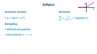
The document discusses output activation and loss functions for neural networks. It provides an overview of common activation functions used for the output layer like sigmoid, tanh, softmax and rectified linear units. It also reviews loss functions like squared error loss and cross entropy loss defined based on the network's output activation. The loss functions guide the weight updates in the network during training to minimize error.

![Cheat Sheet 2
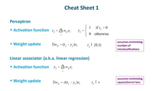
✓ Two layer net (a.k.a. logistic regression)
▪ activation function
▪ weight update
✓ Deep(er) net
▪ activation function same as above
▪ weight update
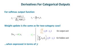
zj = wjixi
i
å yj =
1
1+ exp(-zj )
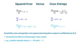
Dwji = e(tj - yj )yj (1- yj )xi tj Î 0,1
[ ]
assumes minimizing
squarederror loss
Dwji = ed j xi d j =
(tj - yj )yj (1- yj ) for output unit
wkjdk
k
å
æ
è
ç
ö
ø
÷ yj (1- yj ) for hidden unit
ì
í
ï
ï
î
ï
ï
assumes minimizing
squarederror loss](https://image.slidesharecdn.com/activationloss1-230922025551-de9936e6/85/activation_loss-1-pdf-3-320.jpg)
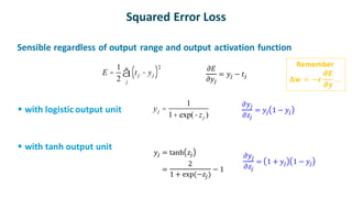

![Cross Entropy Loss
✓ Used when the target output represents a probability distribution
▪ e.g., a single output unit that indicates the classification decision (yes, no) for an
input
Output𝒚 ∈ [𝟎,𝟏] denotesBernoullilikelihoodof class membership
Target 𝒕 indicatestrue class probability(typically0 or 1)
Note: single valuerepresentsprobability distribution over 2 alternatives
✓ Cross entropy, 𝑯, measures distance in bits from predicted distribution to target
distribution
✓
𝐸 = 𝐻 = −𝑡ln 𝑦 − 1 − 𝑡 ln 1 − 𝑦
𝜕𝐸
𝜕𝑦
=
𝑦 − 𝑡
𝑦(1 − 𝑦)](https://image.slidesharecdn.com/activationloss1-230922025551-de9936e6/85/activation_loss-1-pdf-6-320.jpg)