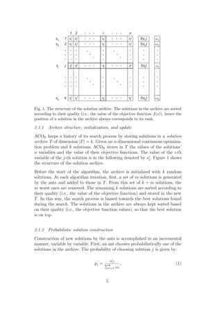
The document describes an extension of Ant Colony Optimization (ACO) called ACOMV that allows it to handle mixed-variable optimization problems containing both continuous and discrete variables. ACOMV uses a solution archive, like ACOR, to probabilistically construct new solutions and guide the search. For ordered discrete variables, it uses a continuous relaxation approach by operating on the indexes of variable values rather than the values themselves. For categorical discrete variables, which have no natural ordering, it handles them natively without assumptions about ordering. The document proposes a new benchmark problem to test whether ACOMV performs better than ACOR on problems with categorical variables, since ACOR relies on ordering assumptions. Preliminary results on this benchmark and other problems are

1. Université Libre de Bruxelles
Institut de Recherches Interdisciplinaires
et de Développements en Intelligence Artificielle
Ant Colony Optimization
for Mixed-Variable Optimization Problems
Krzysztof Socha and Marco Dorigo
IRIDIA – Technical Report Series
Technical Report No.
TR/IRIDIA/2007-019
October 2007

2. IRIDIA – Technical Report Series
ISSN 1781-3794
Published by:
IRIDIA, Institut de Recherches Interdisciplinaires
et de D´veloppements en Intelligence Artificielle
e
´
Universite Libre de Bruxelles
Av F. D. Roosevelt 50, CP 194/6
1050 Bruxelles, Belgium
Technical report number TR/IRIDIA/2007-019
The information provided is the sole responsibility of the authors and
does not necessarily reflect the opinion of the members of IRIDIA. The
authors take full responsability for any copyright breaches that may
result from publication of this paper in the IRIDIA – Technical Report
Series. IRIDIA is not responsible for any use that might be made of
data appearing in this publication.

3. Ant Colony Optimization
for
Mixed-Variable Optimization Problems
Krzysztof Socha and Marco Dorigo
IRIDIA, CoDE, Universit´ Libre de Bruxelles, CP 194/6,
e
Ave. Franklin D. Roosevelt 50, 1050 Brussels, Belgium
http://iridia.ulb.ac.be
Abstract
In this paper, we show how ant colony optimization (ACO) may be used for tack-
ling mixed-variable optimization problems. We show how a version of ACO extended
to continuous domains (ACOR ) may be further used for mixed-variable problems.
We present different approaches to handling mixed-variable optimization problems
and explain their possible uses. We propose a new mixed-variable benchmark prob-
lem. Finally, we compare the results obtained to those reported in the literature for
various real-world mixed-variable optimization problems.
Key words:
ant colony optimization, continuous optimization, mixed-variable optimization,
metaheuristics, engineering problems
1 Introduction
Ant colony optimization (ACO) is a metaheuristic for the approximate solu-
tion of discrete optimization problems that was first introduced in the early
90’s [Dor92,DMC96]. ACO was inspired by the foraging behavior of ant colonies.
When searching for food, ants initially explore the area surrounding their nest
in a random manner. While moving, they leave a chemical pheromone trail on
the ground. As soon as an ant finds a food source, it evaluates the quantity
and the quality of the food and carries some of it back to the nest. During
the return trip, the quantity of pheromone that an ant leaves on the ground
Email addresses: ksocha@ulb.ac.be (Krzysztof Socha), mdorigo@ulb.ac.be
(Marco Dorigo).
Preprint submitted to Elsevier Science 24 August 2007

4. may depend on the quantity and quality of the food. The pheromone trails
guide other ants to the food source. It has been shown in [DAGP90] that the
indirect communication between the ants via pheromone trails let them find
shortest paths between their nest and food sources. The shortest path find-
ing capabilities of real ant colonies are exploited in artificial ant colonies for
solving optimization problems.
While ACO algorithms were originally introduced to solve discrete optimiza-
tion problems, their adaptation to solve continuous optimization problems en-
joys an increasing attention. Early applications of the ants metaphor to contin-
uous optimization include algorithms such as Continuous ACO (CACO) [BP95],
the API algorithm [MVS00], and Continuous Interacting Ant Colony (CIAC) [DS02].
However, all these approaches do not follow the original ACO framework (for
a discussion of this point see [SD06]). Recently, an approach that is closer to
the spirit of ACO for combinatorial problems was proposed in [Soc04,SD06]
and is called ACOR .
In this work, we extend ACOR so that it can be applied to mixed-variable op-
timization problems. Mixed-variable optimization is a combination of discrete
and continuous optimization—that is, the variables being optimized may be
either discrete or continuous. There are several ways of tackling mixed-variable
optimization problems. Some approaches relax the search space, so that it be-
comes entirely continuous [LZ99b,LZ99c,Tur03,GHYC04]. Then, the problem
may be solved using a continuous optimization algorithm. In these approaches,
the values chosen by the algorithms are repaired when evaluating the objec-
tive function, so that they conform to the original search space definition.
In other approaches, the continuous variables are approximated by discrete
values [PK05], and the problem is then tackled using a discrete optimization
algorithm. Alternatively, so called two-phase approaches have been proposed
in the literature [PA92,SB97], where two algorithms (one discrete and one
continuous) are used to solve a mixed-variable optimization problem. Finally,
there are algorithms that try to handle both discrete and continuous variables
natively [DG98,AD01,OS02].
It has been already shown that ACOR may be successfully used for tackling
continuous optimization problems [SD06]. Hence, similarly to other continuos
optimization algorithms, it may be used also for tackling mixed-variable op-
timization problems through relaxation of the discrete constraints. However,
this relies on the assumption that a certain ordering may be defined on the
set of discrete variables’ values. While this assumption is fulfilled in many real
world problems, 1 it is not necessarily always the case. In particular, this is not
true for categorical variables, that is, variables that may assume values associ-
ated with elements of an unordered set. We can intuitively expect that if the
1 Consider for instance pipe diameters: the sizes could be 1 ”, 1 ”, 1”, 1 2 ”, etc., and
4 2
1
the ordering of these values is obvious.
2

5. correct ordering is not known, or does not exist (as in case of categorical vari-
ables), the continuous optimization algorithms may perform poorly. In fact,
the choice of the ordering made by the researcher may affect the performance
of the algorithm.
On the other hand, algorithms that natively handle mixed-variable optimiza-
tion problems are indifferent to the ordering of the discrete variables, as they
do not make any particular assumptions about it. Hence—again intuitively—
we would expect that these algorithms would perform better on problems
containing categorical variables, and that they would not be sensitive to the
particular ordering chosen.
Accordingly, in this paper we test the hypothesis that:
Hypothesis 1.1
Native mixed-variable optimization algorithms are more
efficient than continuous optimization algorithms with
relaxed discrete constraints in the case of mixed-variable
problems containing categorical variables, for which no
obvious ordering exists.
In order to test this hypothesis, we have extended ACOR so that it is able to
handle natively also mixed-variable optimization problems. Additionally, we
need to select a proper benchmark problem. Mixed-variable benchmark prob-
lems may be found in the literature. They often originate from the mechanical
engineering field. Examples include the coil spring design problem [DG98,LZ99c,GHYC04],
the problem of designing a pressure vessel [DG98,GHYC04,ST05], or the ther-
mal insulation systems design [AD01,KAD01]. None of these problems, how-
ever, can be easily parametrized for the purpose of comparing the performance
of a continuous and a mixed-variable algorithm. Because of this, we propose
a new simple yet flexible benchmark problem based on the Ellipsoid function.
We use this benchmark problem for analyzing the performance of two versions
of ACOR —continuous and mixed-variable. Later, we evaluate the performance
of ACOR also on other typical benchmark problems from the literature.
The remainder of this paper is organized as follows. Section 2 presents the
modified ACOR that is able to handle both continuous and mixed-variable
problems. We call it ACOMV . In Section 3, our proposed benchmark is de-
fined, which allows to easily compare the performance of ACOR with that of
ACOMV . The results of this comparison are presented and analyzed. In Sec-
tion 4, ACOR and ACOMV are tested on benchmark problems derived from
real-world problems. The results obtained are also compared to those found
in the literature. Finally, Section 5 summarizes the results obtained, offers
conclusions, and outlines the plans for future work.
3

6. 2 Mixed-Variable ACOR
The extension of ACO to continuous domains—ACOR —has already been de-
scribed in [SD06]. In this paper, we provide an equivalent alternative descrip-
tion that we believe is clearer, shorter, and more coherent. We use this more
compact description of ACOR to introduce its further adaptation to handle
mixed-variable optimization problems.
2.1 ACO for Continuous Domains—ACOR
The ACO metaheuristic finds approximate solutions to an optimization prob-
lem by iterating the following two steps:
(1) Candidate solutions are constructed in a probabilistic way using a prob-
ability distribution over the search space;
(2) The candidate solutions are used to modify the probability distribution
in a way that is deemed to bias future sampling toward high quality
solutions.
ACO algorithms for combinatorial optimization problems make use of a phero-
mone model in order to probabilistically construct solutions. A pheromone
model is a set of so-called pheromone trail parameters. The numerical values
of these pheromone trail parameters (that is, the pheromone values) reflect
the search experience of the algorithm. They are used to bias the solution
construction over time towards the regions of the search space containing high
quality solutions.
In ACO for combinatorial problems, the pheromone values are associated with
a finite set of discrete values related to the decisions that the ants make. This
is not possible in the continuous case. Hence, ACOR uses a solution archive as
a form of pheromone model for the derivation of a probability distribution over
the search space. The solution archive contains a number of complete solutions
to the problem. While a pheromone model in combinatorial optimization can
be seen as an implicit memory of the search history, a solution archive is an
explicit memory. 2
The basic flow of the ACOR algorithm is as follows. As a first step, the solution
archive is initialized. Then, at each iteration a number of solutions is proba-
bilistically constructed by the ants. These solutions may be improved by any
improvement mechanism (for example, local search or gradient techniques).
Finally, the solution archive is updated with the generated solutions. In the
following we outline the components of ACOR in more details.
2 A similar idea was proposed for by Guntsch and Middendorf [GM02] for combi-
natorial optimization problems.
4

7. Fig. 1. The structure of the solution archive. The solutions in the archive are sorted
according to their quality (i.e., the value of the objective function f (s)), hence the
position of a solution in the archive always corresponds to its rank.
2.1.1 Archive structure, initialization, and update
ACOR keeps a history of its search process by storing solutions in a solution
archive T of dimension |T | = k. Given an n-dimensional continuous optimiza-
tion problem and k solutions, ACOR stores in T the values of the solutions’
n variables and the value of their objective functions. The value of the i-th
variable of the j-th solution is in the following denoted by si . Figure 1 shows
j
the structure of the solution archive.
Before the start of the algorithm, the archive is initialized with k random
solutions. At each algorithm iteration, first, a set of m solutions is generated
by the ants and added to those in T . From this set of k + m solutions, the
m worst ones are removed. The remaining k solutions are sorted according to
their quality (i.e., the value of the objective function) and stored in the new
T . In this way, the search process is biased towards the best solutions found
during the search. The solutions in the archive are always kept sorted based
on their quality (i.e., the objective function values), so that the best solution
is on top.
2.1.2 Probabilistic solution construction
Construction of new solutions by the ants is accomplished in an incremental
manner, variable by variable. First, an ant chooses probabilistically one of the
solutions in the archive. The probability of choosing solution j is given by:
ωj
pj = k , (1)
r=1 ωr
5

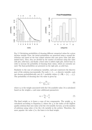
8. where ωj is a weight associated with solution j. The weight may be calculated
using various formulas depending on the problem tackled. In the remainder of
this paper we use a Gaussian function g(µ, σ) = g(1, qk), which was also used
in our previous work [SD06]:
1 −(j−1)2
ωj = √ e 2q 2 k2 , (2)
qk 2π
where, q is a parameter of the algorithm and k is the size of the archive. The
mean of the Gaussian function is set to 1, so that the best solution has the
highest weight.
The choice of the Gaussian function was motivated by its flexibility and non-
linear characteristic. Thanks to its non-linearity, it allows for a flexible control
over the weights. It is possible to give higher probability to a few leading
solutions, while significantly reducing the probability of the remaining ones.
Once a solution is chosen, an ant may start constructing a new solution. The
ant treats each problem variable i = 1, ..., n separately. It takes the value si
j
of the variable i of the chosen j-th solution and samples its neighborhood.
This is done using a probability density function (PDF). Again, as in the case
of choosing the weights, many different functions may be used. A PDF P (x)
must however satisfy the condition:
∞
P (x)dx = 1. (3)
−∞
In this work, similarly to earlier publications presenting ACOR [SD06], we use
as PDF the Gaussian function:
1 (x−µ)2
P (x) = g(x, µ, σ) = √ e− 2σ2 . (4)
σ 2π
The function has two parameters that must be defined: µ, and σ. When con-
sidering variable i of solution j, we assign µ ← si . Further, we assign σ:
j
k
|si − si |
r j
σ←ξ . (5)
r=1 k−1
which is the average distance between the i-th variable of the solution sj
and the i-th variables of the other solutions in the archive, multiplied by a
parameter ξ 3 .
3 Parameter ξ has an effect similar to that of the pheromone evaporation rate in
ACO. The higher the value of ξ, the lower the convergence speed of the algorithm.
While the pheromone evaporation rate in ACO influences the long term memory—
i.e., the worst solutions are forgotten faster—ξ in ACOR influences the way the long
6

9. This whole process is repeated for each dimension i = 1, ..., n in turn by each
of the m ants.
2.2 ACOMV for Mixed-Variable Optimization Problems
ACOMV extends ACOR allowing to declare each variable of the considered
problem as continuous, ordered discrete, or categorical discrete. Continuous
variables are treated as in the original ACOR , while discrete variables are
treated differently. The pheromone representation (i.e., the solution archive)
as well as the general flow of the algorithm do not change. Hence, we focus
here on presenting how the discrete variables are handled.
If there are any ordered discrete variables defined, ACOMV uses a continuous-
relaxation approach. The natural ordering of the values for these variables may
have little to do with their actual numerical values (and they may even not
have numerical values, e.g., x ∈ {small, big, huge}). Hence, instead of operat-
ing on the actual values of the ordered discrete variables, ACOMV operates on
their indexes. The values of the indexes for the new solutions are generated by
the algorithm as real numbers, as it is the case for the continuous variables.
However, before the objective function is evaluated, the continuous values are
rounded to the nearest valid index, and the value at that index is then used
for the objective function evaluation.
Clearly, at the algorithm level, ACOMV ≡ACOR in this case. However, things
change when the problem includes categorical discrete variables, as for this
type of variables there is no pre-defined ordering. This means that the in-
formation about the ordering of the values in the domain may not be taken
into consideration. The values for these variables need to be generated with
a different method—one that is closer to the regular combinatorial ACO. We
present the method used by ACOMV in the following section.
2.2.1 Solution Construction for Categorical Variables
In standard ACO (see [DS04]), solutions are constructed from solution com-
ponents using a probabilistic rule based on the pheromone values. Differently,
in ACOMV there are no static pheromone values, but a solution archive. As in
standard ACO, in ACOMV the construction of solutions for discrete variables
is done by choosing the components, that is, the values for each of the discrete
decision variables. However, since the static pheromone values of standard
ACO are replaced by the solution archive, the actual probabilistic rule used
has to be modified.
term memory is used—i.e., the new solutions are considered closer to known good
solutions.
7

10. Final Probabilities
f c d e b
0.30
0.12
0.20
0.08
probability
probability
0.10
0.04
0.00
0.00
1 2 3 4 5 6 7 8 9 a b c d e f g
ranks categories
Fig. 2. Calculating probabilities of choosing different categorical values for a given
decision variable. First, the initial probabilities are generated using a normal dis-
tribution and based on the best ranked solution that uses given value (left plot,
dashed bars). Then, they are divided by the number of solutions using this value
(left plot, solid bars), and finally a fixed value is added (right plot, dotted bars) in
order to increase the probability of choosing those values, which are currently not
used. The final probabilities are presented on the right plot, as solid bars.
Similarly to the case of continuous variables, each ant constructs the discrete
part of the solution incrementally. For each i = 1, ..., n discrete variable, each
ant chooses probabilistically one of ci available values vli ∈ Di = {v1 , ..., vci }.
i i
The probability of choosing the l-th value is given by:
wl
oi =
l c , (6)
r=1 wr
where wl is the weight associated with the l-th available value. It is calculated
based on the weights ω and some additional parameters:
ωjl q
wl = i
+ . (7)
ul η
The final weight wl is hence a sum of two components. The weight ωjl is
calculated according to Equation 2, where the jl is the index of the highest
quality solution that uses value vli for the i-th variable. In turn, ui is the number
l
of solutions using value vli for the i-th variable in the archive. Therefore, the
more popular the value vli is, the lower is its final weight.
8

11. The second component is a fixed value (i.e., it does not depend on the value
vli chosen): η is the number of values vli from the ci available ones that are
unused by the solutions in the archive, and q is the same parameter of the
algorithm that was used in Equation 2.
ω
The graphical representation of how the first component ujil is calculated is
l
presented on the left plot of Figure 2. The dashed bars indicate the values
of the weights ωjl obtained for the best solutions using the available values. 4
The solid bars represent the weights ωjl divided by the respective number of
solutions ui that use values vli . It is shown for the available set of categorical
l
values used, vli ∈ {a, b, c, d, e, f, g} in this example.
Some of the available categorical values vl may be unused for a given i-th
decision variable in all the solutions in the archive. Hence, their initial weight
is zero. In order to enhance exploration and to prevent premature convergence,
in such a case, the final weights w are further modified by adding to all of
them the second component. Its value depends on the parameter q and on the
number of unused categorical values ηi , as shown in Equation 7.
The right plot in Figure 2 presents the normalized final probabilities for an
example in which the solution archive has size k = 10, and where the set
of categorical values is {a, b, c, d, e, f, g}, with values {a} and {g} unused by
the current decision variable. The dotted bars show the value of q/η added
to all the solutions, and the solid bars show the final resulting probabilities
associated with each of the available categories. These probabilities are then
used to generate the value of the i-th decision variable for the new solutions.
3 Simple Benchmark Problem
Benchmark problems used in the literature to evaluate the performance of
mixed-variable optimization algorithms are typically real-world mechanical
engineering problems. They include among others: pressure vessel design, coil
spring design, or thermal insulation system design problems. Although we also
use these problems in Section 4, they are not very well suited for the detailed
investigation of the performance of an algorithm. This is because their search
space is not clearly defined and easy to analyze. Additionally, the objective
functions of these problems cannot be manipulated easily in order to check the
sensitivity of the algorithm to particular conditions. Hence, such test problems
do not represent a sufficiently controlled environment for the investigation of
the performance of an algorithm.
In order to be able to flexibly compare ACOR using the continuous relaxation
4 If a given value is not used, the associated index is indefinite, and thus its initial
weight is zero.
9

12. approach with the native mixed-variable ACOMV algorithm, we have designed
a new mixed-variable benchmark problem. We have based it on a randomly
rotated Ellipsoid function:

n 
 x ∈ (−3, 7)n ,
i−1
fEL (x) = (β n−1 zi )2 , (8)

 z = Ax,
i=1
where β is the coefficient defining the scaling of each dimension of the ellip-
soid, n is number of dimensions and A is a random normalized n-dimensional
rotation matrix. In order to make it easier to analyze and visualize the results,
we have limited ourselves to the two dimensional case (n = 2). 5
In order to transform this continuous optimization problem into a mixed-
variable one, we have divided the continuous domain of variable x1 ∈ (−3, 7)
into a set of discrete values, T = {θ1 , θ2 , ..., θt } : θi ∈ (−3, 7). This results in
the following mixed-variable test function:


 x ∈ T,
 1



2 2
fELM V (x) = z1 + β · z2 , (9)
 x2 ∈ (−3, 7),




 z = Ax.
The set T is created by choosing t uniformly spaced values from the original
domain (−3, 7) in such a way that ∃i=1,...,t θi = 0. This way, it is always
possible to find the optimum fELM V (0, 0) = 0, regardless of the chosen value
for t.
3.1 Experimental Setup
We have compared ACOR and ACOMV on two experimental setups of our
test problem. We used β = 100, as this is the value most often reported in
the literature for the ellipsoid function. The two setups simulate two types of
mixed-variable optimization problems: (i) with ordered discrete variables, and
(ii) with categorical variables.
In the first setup, the discrete intervals for variable x1 are naturally ordered.
Such a setup simulates a problem where the ordering of the discrete variables
may be easily defined. The left plot in Figure 3 shows how the algorithm sees
such a naturally ordered rotated ellipsoid function, with discrete x1 variable. 6
The test function is presented as the ACOR algorithm sees it—as a set of points
5 Higher dimensional problems are discussed in Section 4.
6 Please note that Figure 3 uses the value of β = 5, as it is clearer for visualization.
This simply means that the ellipsoid is less flat and more circle-like.
10

13. 6 Natural Random
6
4
4
X2
X2
2
2
0
0
−2
−2
−2 0 2 4 6 −2 0 2 4 6
X1 X1
Fig. 3. Randomly rotated ellipsoid function (β = 5) with discrete variable
x1 ∈ T, |T| = t = 30. The left plot presents the case in which the natural or-
dering of the intervals is used, while the right one presents the case in which a
random ordering is used.
representing different solutions found by the ants and stored in the solution
archive. The darker the point, the higher the quality of the solution.
In the second setup, the intervals are ordered randomly, that is, for each
run of the algorithm a different ordering was generated. This setup allows to
investigate how the algorithm performs when the optimum ordering of the
intervals is not well defined or unknown. The right plot of Figure 3 shows how
the algorithm sees such modified problem for a given single random ordering.
Clearly, compared to the natural ordering, the problem appears to be quite
different.
For both setups, we have run both ACOR and ACOMV . We have tested the
two algorithms on both test setups for a different number t of intervals for
variable x1 . For fewer number of intervals, the problem is less continuous, but
the probability of choosing the wrong interval is relatively small. At the same
time, since the domain is always the same, the size of the intervals is larger,
and ACOR may get stuck more easily. The more intervals are used, the more
the problem resembles a continuos problem, up to t → ∞, when it would
become a true continuos optimization problem.
11

14. Table 1
Summary of the parameters used by ACOR and ACOMV .
Parameter Symbol ACOR ACOMV
number of ants m 2 2
speed of convergence ξ 0.3 0.7
locality of the search q 0.1 0.8
archive size k 200 50
3.2 Parameter Tuning
In order to ensure a fair comparison of the two algorithms, we have applied an
identical parameter tuning procedure to both: the F-RACE method [BSPV02,Bir05].
We have defined 168 candidate configurations of parameters for each of the
algorithms. Then, we have run them on 150 instances of the test problem,
which differed in terms of number of intervals used (t ∈ {10, 20, 50}), and of
their ordering (we used always random ordering for parameter tuning). We
used 50 instances for each chosen number of intervals.
The summary of the parameters chosen is given in Table 1.
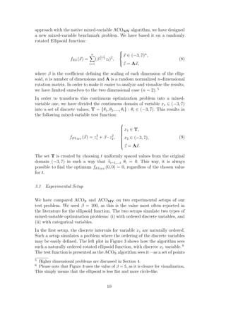
3.3 Results
For each version of the benchmark problem, we have evaluated the perfor-
mance of ACOR and ACOMV for different numbers of intervals t ∈ {2, 4, 8, 11,
13, 15, 16, 18, 20, 22, 32, 38, 50}. We have done 200 independent runs of each al-
gorithm for each version of the benchmark problem and for each number of
intervals tested.
Figure 4 presents the performance of ACOR (thick solid line) and ACOMV
(thinner solid line) on the benchmark problem with naturally ordered discrete
intervals. The left plot presents the distributions boxplots of the results for
a representative sample (t = 8, 20, 50) of the number of intervals used. The
boxplots marked as c.xx were produced from results obtained with ACOR ,
and the boxplots marked as m.xx were produced from results obtained with
ACOMV . The xx is replaced by the actual number of intervals used. Note
that the y-axis is scaled to the range [0, 1] for readability reasons (this causes
some outliers to be not visible). The right plot presents an approximation
(using smooth splines with five degrees of freedom) of the mean performance,
as well as the actual mean values measured for various numbers of intervals.
Additionally, we indicate the standard error of the mean (also using smooth
splines).
12

15. 1.0 Performance Depending on the Number of Intervals − Natural Ordering
1.0
continuous relaxation approach
native mixed approach
0.8
0.8
0.6
0.6
mean f(x)
f(x)
0.4
0.4
0.2
0.2
0.0
0.0
c.8 m.8 c.20 m.20 c.50 m.50 1 2 5 10 20 50
cont. and mixed ACO for 8, 20, and 50 intervals number of intervals
Fig. 4. Performance of ACOR and ACOMV on a discretized randomly rotated El-
lipsoid function (n = 2) with natural ordering of the intervals. The left plot shows
the distribution of the results of ACOR (c) and ACOMV (m) for t = {8, 20, 50}.
The right plot shows the mean performance of both algorithms with regard to the
number of intervals used. The dotted lines indicate the standard error of the mean
and the circles the actual means measured for different numbers of intervals. Note
that the left plot has been scaled for readability reasons, which makes some outliers
(that strongly affect the mean performance shown on the right plot) not visible.
Figure 5 presents in turn the performance of ACOR and ACOMV on the bench-
mark problem with randomly ordered intervals. It is organized similarly to
Figure 4.
A comparison of Figures 4 and 5 reveals that, while the performance of
ACOMV does not change significantly, ACOR performs much better in the
case of natural ordering of the intervals. In this case, the mean performance
of ACOR is inferior to the one of ACOMV when t < 18. As the number of
intervals used increases, the performance of ACOR improves, and eventually
(for t > 20) it becomes better than ACOMV .
Clearly, the performance of ACOR is different for a small or for a large number
of intervals. For a small number of intervals, the mean performance of ACOR
is influenced by the large size of the intervals. If the algorithm gets stuck in
the wrong interval, the best value it can find there is much worse than the
optimum one. Hence, although this happens quite rarely, this causes worse
mean performance. The more intervals are used, the closer the problem re-
sembles a continuous one. The size of intervals becomes smaller, and ACOR is
less likely to get stuck in a wrong one. Hence, for larger number of intervals
used, ACOR ’s performance improves.
The mean performance of ACOR on the version of the benchmark problem with
13

16. 1.0 Performance Depending on the Number of Intervals − Random Ordering
1.0
continuous relaxation approach
native mixed approach
0.8
0.8
0.6
0.6
mean f(x)
f(x)
0.4
0.4
0.2
0.2
0.0
0.0
c.8 m.8 c.20 m.20 c.50 m.50 1 2 5 10 20 50
cont. and mixed ACO for 8, 20, and 50 intervals number of intervals
Fig. 5. Performance of ACOR and ACOMV on a discretized randomly rotated Ellip-
soid function (n = 2) with random ordering of the intervals. The left plot presents
the distribution of the results of ACOR (c) and ACOMV (m) for t = {8, 20, 50}. The
right plot shows the analysis of mean performance of both algorithms with regard
to the number of intervals used. The dotted lines indicate the standard error of the
mean, and the circles the actual means measured for different numbers of intervals.
Please note that the left plot has been scaled for readability reasons, which makes
some outliers (that strongly affect the mean performance shown on the right plot)
not visible.
randomly ordered intervals follows a similar pattern, but is generally worse. For
a small number of intervals, the mean performance is penalized by their large
size. With increasing number of intervals, the performance further degrades
due to the lack of natural ordering—the search space contains discrete traps,
with which ACOR does not deal very well. For t > 20, the mean performance
begins to improve again, as there is a higher probability of finding a discrete
interval reasonably close in quality to the optimal one. It is important to
notice that, while in the case of natural ordering the median performance is
systematically very good for any number of intervals, in the case of random
ordering the median performance of ACOR decreases with the increase of the
number of intervals. Also, the mean performance of ACOR remains inferior to
ACOMV for any number of intervals tested.
Contrary to ACOR , the mean performance of ACOMV does not differ for the
two versions of the benchmark problem. This is consistent with the initial
hypothesis, since the ordering of the intervals should not matter for a native
mixed-variable algorithm. ACOMV is always able to find an interval that is
reasonably close in quality to the optimal one. Its efficiency depends only
on the number of intervals available. The more there are intervals, the more
difficult it becomes to find the optimal one. This is why the mean performance
14

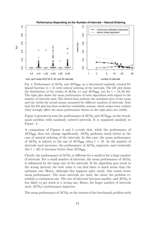
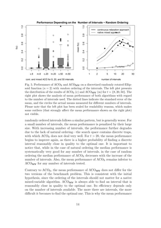
17. of ACOMV decreases slightly with the increase of the number of intervals.
3.4 Discussion
Our initial hypothesis that the ordering of the discrete intervals should not
have impact on the performance of the native mixed-variable optimization
algorithm appears to hold. The mean performance of ACOMV is better than
ACOR , when the ordering is not natural. These results suggest that ACOMV
should perform well also on other real-world and benchmark problems con-
taining categorical variables.
In order to further asses the performance of ACOMV on various mixed-variable
optimization problems, we tackle them using both ACOR and ACOMV in the
next section. We also compare the results obtained with those reported in the
literature, so that the results obtained by ACOR and ACOMV may be put in
perspective.
4 Results on Various Benchmark Problems
In many industrial processes and problems some parameters are discrete and
other continuous. This is why problems from the area of mechanical design are
often used as benchmarks for mixed-variable optimization algorithms. Popu-
lar examples include truss design [SBR94,Tur03,PK05,ST05], coil spring de-
sign [DG98,LZ99c,GHYC04], pressure vessel design [DG98,GHYC04,ST05],
welded beam design [DG98], and thermal insulation systems design [AD01,KAD01].
In order to illustrate the performance of ACOR and ACOMV on real-world
mixed-variable problems, we use a subset of these problems. In particular,
in the following sections, we present the performance of ACOR and ACOMV
on the pressure vessel design problem, the coil spring design problem, and
the thermal insulation system design problem. Also, we compare the results
obtained with those reported in the literature.
4.1 Pressure Vessel Design Problem
The first engineering benchmark problem that we tackle is the problem of
designing a pressure vessel. The pressure vessel design (PVD) problem has
been used numerous times as a benchmark for mixed-variable optimization
algorithms [San90,DG98,LZ99a,GHYC04,ST05].
15

18. Fig. 6. Schematic of the pressure vessel to be designed.
Table 2
Constraints for the three cases (A, B, and C) of the pressure vessel design problem.
No Case A Case B Case C
g1 Ts − 0.0193 R ≥ 0
g2 Th − 0.00954 R ≥ 0
g3 π R2 L + 4 π R3 − 750 · 1728 ≥ 0
3
g4 240 − L ≥ 0
g5 1.1 ≤ Ts ≤ 12.5 1.125 ≤ Ts ≤ 12.5 1 ≤ Ts ≤ 12.5
g6 0.6 ≤ Th ≤ 12.5 0.625 ≤ Th ≤ 12.5
g7 0.0 ≤ R ≤ 240.0
g8 0.0 ≤ L ≤ 240.0
4.1.1 Problem Definition
The problem requires designing a pressure vessel consisting of a cylindrical
body and two hemispherical heads such that the cost of its manufacturing is
minimized subject to certain constraints. The schematic picture of the vessel
is presented in Figure 6. There are four variables for which values must be
chosen: the thickness of the main cylinder Ts , the thickness of the heads Th ,
the inner radius of the main cylinder R, and the length of the main cylinder
L. While variables R and L are continuous, the thickness for variables Ts and
Th may be chosen only from a set of allowed values, these being the integer
multiplies of 0.0625 inch.
There are numerous constraints for the choice of the values of the variables. In
fact, there are three distinctive cases (A, B, and C) defined in the literature.
These cases differ by the constraints posed on the thickness of the steel used for
the heads and the main cylinder. Since each case results in a different optimal
solution, we present here all three of them. Table 2 presents the required
constrains for all three cases.
16

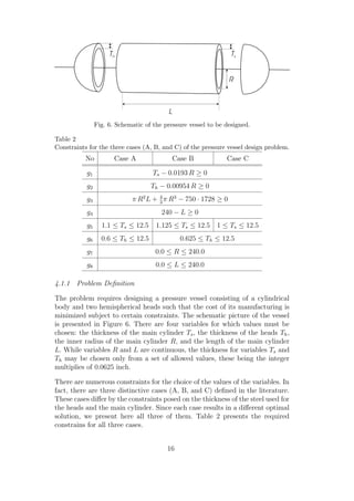
19. The objective function represents the manufacturing cost of the pressure ves-
sel. It is a combination of material cost, welding cost, and forming cost. Using
rolled steel plate, the main cylinder is to be made in two halves that are joined
by two longitudinal welds. Each head is forged and then welded to the main
cylinder. The objective function is the following:
f (Ts , Th , R, L) = 0.6224 Ts RL + 1.7781 Th R2 + 3.1611 Ts2 L + 19.84 Ts2 R. (10)
The coefficients used in the objective function, as well as the constraints, come
from conversion of units from imperial to metric ones. The original problem
defined the requirements in terms of imperial units, that is, the working pres-
sure of 3000 psi and the minimum volume of 750 ft3 . For more details on the
initial project formulation, as well as on how the manufacturing cost of the
pressure vessel is calculated, we refer the interested reader to [San90].
4.1.2 Experimental Setup
Most benchmarks found in the literature set to 10, 000 the number of function
evaluations on which the algorithms are evaluated. Accordingly, we use 10, 000
function evaluations as stopping criterion for both ACOR and ACOMV .
The constraints defined in the PVD problem were handheld in a rather simple
manner. The objective function was defined in such a way that if any of the
constraints was violated, the function returns an infinite value. In this way
feasible solutions are always better than infeasible ones.
For each of the cases A, B, and C, we have performed 100 independent runs
for ACOR and ACOMV in order to asses the robustness of the performance.
4.1.3 Parameter Tuning
In order to ensure a fair comparison of ACOR and ACOMV , we have used
the F-RACE method for tuning the parameters. The parameters selected by
F-RACE are listed in Table 3. Note that the same parameters were selected
for all the three cases of the PVD problem.
4.1.4 Results
The pressure vessel design problem has been tackled by numerous algorithms
in the past. The results of the following algorithms are available in the litera-
ture:
• nonlinear integer and discrete programming [San90] (cases A and B),
• mixed integer-discrete-continuous programming [FFC91] (cases A and B),
17

20. Table 3
Summary of the parameters chosen for ACOR and ACOMV for the PVD problem.
Parameter Symbol ACOR ACOMV
number of ants m 2 2
speed of convergence ξ 0.9 0.8
locality of the search q 0.05 0.3
archive size k 50 50
Table 4
Results for Case A of the pressure vessel design problem. For each algorithm are
given the best value, the success rate (i.e., how often the best value was reached),
and the number of function evaluations allowed. Note that, in some cases, the num-
ber of evaluations allowed was not indicated in the literature. Also, for the ACO
algorithms, the mean number of evaluations of the successful runs is given in paren-
theses.
[San90] [FFC91] [LZ99a] ACOR ACOMV
f∗ 7867.0 7790.588 7019.031 7019.031 7019.031
success rate 100% 99% 89.2% 100% 28%
# of function eval. - - 10000 10000 10000
(3037) (6935)
• sequential linearization approach [LP91] (case B),
• nonlinear mixed discrete programing [LC94] (case C),
• genetic algorithm [WC95] (case B),
• evolutionary programming [CW97] (case C),
• evolution strategy [TC00] (case C),
• differential evolution [LZ99a] (cases A, B, and C),
• combined heuristic optimization approach [ST05] (case C),
• hybrid swarm intelligence approach [GHYC04] (case B).
For the sake of completeness, we have run our algorithms on all the three cases
of the PVD problem. Tables 4, 5, and 6 summarize the results found in the
literature and those obtained by ACOR and ACOMV . Each table provides the
best value found (rounded to three digits after the decimal point), the success
rate—that is, the percentage of the runs, in which at least the reported best
value was found, and the number of function evaluations allowed. We have
performed 100 independent runs for both ACOR and ACOMV .
Based on the results obtained, it may be concluded that both ACOR and
ACOMV are able to find the best currently known value for all three cases of
18

21. Table 5
Results for Case B of the pressure vessel design problem. For each algorithm are
given the best value, the success rate (i.e., how often the best value was reached),
and the number of function evaluations allowed. Note that, in some cases, the num-
ber of evaluations allowed was not indicated in the literature. Also, for the ACO
algorithms, the mean number of evaluations of the successful runs is given in paren-
theses.
[San90] [LP91] [WC95] [LZ99a] [GHYC04] ACOR ACOMV
f∗ 7982.5 7197.734 7207.497 7197.729 7197.9 7197.729 7197.729
success rate 100% 90.2% 90.3% 90.2% - 100% 35%
# of function eval. - - - 10000 - 10000 10000
(3124) (6998)
Table 6
Results for Case C of the pressure vessel design problem. For each algorithm are
given the best value, the success rate (i.e., how often the best value was reached),
and the number of function evaluations allowed. Note that, in some cases, the num-
ber of evaluations allowed was not indicated in the literature. Also, for the ACO
algorithms, the mean number of evaluations of the successful runs is given in paren-
theses.
[LC94] [CW97] [TC00] [LZ99a] [ST05] ACOR ACOMV
f∗ 7127.3 7108.616 7006.9 7006.358 7006.51 7006.358 7006.358
success rate 100% 99.7% 98.3% 98.3% - 100% 14%
# of function eval. - - 4800 10000 10000 10000 10000
(3140) (6927)
the PVD problem. Additionally, ACOR is able to do so in just over 3,000 objec-
tive function evaluations on average, while maintaining 100% success rate. On
the other hand, ACOMV , although also able to find the best known solution
for all the three cases of the PVD problem, it does so only in about 30% of
the runs within the 10,000 evaluations of the objective function. Hence, on the
PVD problem ACOMV performs significantly worse than ACOR , which is con-
sistent with the initial hypothesis that ACOR performs better than ACOMV
when the optimization problem includes no categorical variables.
4.2 Coil Spring Design Problem
The second benchmark problem that we considered is the coil spring design
(CSD) problem [San90,DG98,LZ99c,GHYC04]. This is another popular bench-
mark used for comparing mixed-variable optimization algorithms.
19

22. Fig. 7. Schematic of the coil spring to be designed.
4.2.1 Problem Definition
The problem consists in designing a helical compression spring that will hold
an axial and constant load. The objective is to minimize the volume of the
spring wire used to manufacture the spring. A schematic of the coil spring
to be designed is shown in Figure 7. The decision variables are the number
of spring coils N , the outside diameter of the spring D, and the spring wire
diameter d. The number of coils N is an integer variable, the outside diameter
of the spring D is a continuous one, and finally, the spring wire diameter is a
discrete variable, whose possible values are given in Table 7.
The original problem definition [San90] used imperial units. In order to have
comparable results, all subsequent studies that used this problem [DG98,LZ99c,GHYC04]
continued to use the imperial units; so did we.
The spring to be designed is subject to a number of design constraints, which
are defined as follows:
• The maximum working load, Fmax = 1000.0 lb.
• The allowable maximum shear stress, S = 189000.0 psi.
Table 7
Standard wire diameters available for the spring coil.
Allowed wire diameters [inch]
0.0090 0.0095 0.0104 0.0118 0.0128 0.0132
0.0140 0.0150 0.0162 0.0173 0.0180 0.0200
0.0230 0.0250 0.0280 0.0320 0.0350 0.0410
0.0470 0.0540 0.0630 0.0720 0.0800 0.0920
0.1050 0.1200 0.1350 0.1480 0.1620 0.1770
0.1920 0.2070 0.2250 0.2440 0.2630 0.2830
0.3070 0.3310 0.3620 0.3940 0.4375 0.5000
20

23. • The maximum free length, lmax = 14.0 in.
• The minimum wire diameter, dmin = 0.2 in.
• The maximum outside diameter of the spring, Dmax = 3.0 in.
• The pre-load compression force, Fp = 300.0 lb.
• The allowable maximum deflection under pre-load, σpm = 6.0 in.
• The deflection from pre-load position to maximum load position, σw =
1.25 in.
• The combined deflections must be consistent with the length, that is, the
spring coils should not touch each other under the maximum load at which
the maximum spring deflection occurs.
• The shear modulus of the material, G = 11.5 · 106 .
• The spring is guided, so the buckling constraint is bypassed.
• The outside diameter of the spring, D, should be at least three times greater
than the wire diameter, d, to avoid lightly wound coils.
These design constraints may be formulated into a set of explicit constraints,
listed in Table 8. The following symbols are used in the constraints definition:
4 D −1 0.615 d
Cf = d
4 D −4
+ D
d
Gd4
K= 8 N D3
(11)
σp = Fp
K
Fmax
lf = K
+ 1.05(N + 2)d
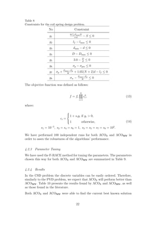
The cost function to be minimized computes the volume of the steel wire as
a function of the design variables:
π Dd2 (N + 2)
fc (N, D, d) = (12)
4
4.2.2 Experimental Setup
Most of the research on the CSD problem reported in the literature focused on
finding the best solution. Only the recent work by Lampinen and Zelinka [LZ99a]
gave some attention to the number of function evaluations used to reach the
best solution. They used 8,000 function evaluations. In order to obtain results
that could be compared, this was used also used for both ACOR and ACOMV .
The constraints defined in the CSD problem were handled with the use of a
penalty function, similarly to the way it was done by Lampinen and Zelinka [LZ99a].
21

24. Table 8
Constraints for the coil spring design problem.
No Constraint
8 Cf Fmax D
g1 πd
−S ≤0
g2 lf − lmax ≤ 0
g3 dmin − d ≤ 0
g4 D − Dmax ≤ 0
D
g5 3.0 − d
≤0
g6 σp − σpm ≤ 0
Fmax −Fp
g7 σp + K
+ 1.05(N + 2)d − lf ≤ 0
Fmax −Fp
g8 σw − K
≤0
The objective function was defined as follows:
8
f = fc c3 ,
i (13)
i=1
where:


 1 + si gi if gi > 0,
ci = 
 1 otherwise, (14)
s1 = 10−5 , s2 = s4 = s6 = 1, s3 = s5 = s7 = s8 = 102 .
We have performed 100 independent runs for both ACOR and ACOMV in
order to asses the robustness of the algorithms’ performance.
4.2.3 Parameter Tuning
We have used the F-RACE method for tuning the parameters. The parameters
chosen this way for both ACOR and ACOMV are summarized in Table 9.
4.2.4 Results
In the CSD problem the discrete variables can be easily ordered. Therefore,
similarly to the PVD problem, we expect that ACOR will perform better than
ACOMV . Table 10 presents the results found by ACOR and ACOMV , as well
as those found in the literature.
Both ACOR and ACOMV were able to find the current best known solution
22

25. Table 9
Summary of the parameters chosen for ACOR and ACOMV for the CSD problem.
Parameter Symbol ACOR ACOMV
number of ants m 2 2
speed of convergence ξ 0.8 0.2
locality of the search q 0.06 0.2
archive size k 120 120
Table 10
Results for the coil spring design problem. For each algorithm are given the best
value, the success rate (i.e., how often the best value was reached), and the number
of function evaluations allowed. Note that, in some cases, the number of evaluations
allowed was not indicated in the literature.
[San90] [WC95] [LZ99a] ACOR ACOMV
f∗ 2.7995 2.6681 2.65856 2.65856 2.65856
success rate 100% 95.3% 95.0% 82% 39%
# of function eval. - - 8000 8000 8000
of the CSD problem. ACOR again performed better than ACOMV . Both were
performing better (in terms of quality of the solutions found) than many
methods reported in literature. ACOR was a bit less robust (lower success rate)
than the differential evolution (DE) used by Lampinen and Zelinka [LZ99a].
The results obtained by ACOR and ACOMV for the coil spring design problem
are consistent with the findings for pressure vessel design. The variables of the
coil spring design problem may be easily ordered and ACOR performs better
than ACOMV , as expected. ACOR was run with the same number of function
evaluations as the DE used by Lampinen and Zelinka. The best result is the
same, but while in the PVD problem ACOR had a higher success rate than
DE [LZ99a] (as well as a faster convergence), in the case of the CSD problem,
the success rate is slightly lower than that of DE.
4.3 Designing Thermal Insulation System
The third engineering problem that we used to test our algorithms was the
thermal insulation system design (TISD) problem. The choice was due to the
fact that this is one of the few benchmark problems used in the literature
that deals with categorical variables—that is, variables which have no natural
ordering.
Various types of thermal insulation systems have been tackled and discussed
in the literature. Hilal and Boom [HB77] considered cryogenic engineering
23

26. applications in which mechanical struts are necessary in the design of solenoids
for superconducting magnetic energy storage systems. In this case, vacuum is
ruled out as an insulator because the presence of a material is always necessary
between the hot and the cold surfaces in order to support mechanical loads.
Hilal and Boom used only few intercepts in their studies (up to three), and they
considered only one single material for all the layers between the intercepts.
More recently, cryogenic systems of space borne magnets have been studied.
The insulation efficiency of a space borne system ensures that the available
liquid helium used for cooling the intercepts evaporates with minimum rate
during the mission. Some studies [MHM89] focused on optimizing the inlet
temperatures and flow rates of the liquid helium for a predefined number of
intercepts and insulator layers. Others [YOY91] studied the effect of the num-
ber of intercepts and the types of insulator on the temperature distribution
and insulation efficiency. Yet others [LLMB89] considered different substances
such as liquid nitrogen or neon for cooling the intercepts and compared dif-
ferent types of insulators.
In all the studies mentioned so far, the categorical variables describing the
type of insulators used in different layers were not considered as optimization
variables, but rather as parameters. This is due to the fundamental property
of categorical variables—there is no particular ordering defined on the set of
available materials, and hence they may not be relaxed to be handheld as
regular continuous optimization variables. The algorithms used by the before
mentioned studies did not allow to handle such categorical variables. Only the
more recent work of Kokkolaras et al. [KAD01] propose a mixed-variable pro-
gramming (MVP) algorithm, which is able to handle such categorical variables
properly.
In this section, we show that, thanks to the fact that ACOMV can also handle
natively categorical variables, it performs comparably to MVP on the thermal
insulation system design problem, and outperforms significantly ACOR , which
further confirms our initial Hypothesis 1.1.
4.3.1 Problem Definition
In our work, we use the definition of thermal insulation system as proposed
by Hilal and Boom [HB77], and later also used by Kokkolaras et al. [KAD01].
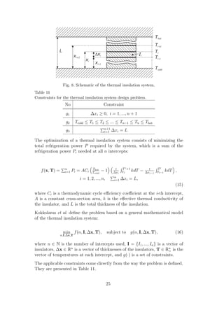
Thermal insulation systems use heat intercepts to minimize the heat flow from
a hot to a cold surface. The cooling temperature Ti is a control imposed at
the i = 1, 2, ..., n locations xi to intercept the heat. The design configuration
of such a multi-intercept thermal insulation system is defined by the number
of intercepts, their locations, temperatures, and types of insulators placed
between each pair of adjacent intercepts. Figure 8 presents the schematic of a
thermal insulation system.
24

27. Fig. 8. Schematic of the thermal insulation system.
Table 11
Constraints for the thermal insulation system design problem.
No Constraint
g1 ∆xi ≥ 0, i = 1, ..., n + 1
g2 Tcold ≤ T1 ≤ T2 ≤ ... ≤ Tn−1 ≤ Tn ≤ Thot
n+1
g3 i=1 ∆xi = L
The optimization of a thermal insulation system consists of minimizing the
total refrigeration power P required by the system, which is a sum of the
refrigeration power Pi needed at all n intercepts:
n Thot 1 T i +1 1 Ti
f (x, T) = i=1 Pi = ACi Tcold
−1 ∆xi Ti kdT − ∆xi−1 Ti−1 kdT ,
n
i = 1, 2, ..., n, i=1 ∆xi = L,
(15)
where Ci is a thermodynamic cycle efficiency coefficient at the i-th intercept,
A is a constant cross-section area, k is the effective thermal conductivity of
the insulator, and L is the total thickness of the insulation.
Kokkolaras et al. define the problem based on a general mathematical model
of the thermal insulation system:
min f (n, I, ∆x, T), subject to g(n, I, ∆x, T), (16)
n,I,∆x,T
where n ∈ N is the number of intercepts used, I = {I1 , ..., In } is a vector of
insulators, ∆x ∈ Rn is a vector of thicknesses of the insulators, T ∈ Rn is the
+
vector of temperatures at each intercept, and g(·) is a set of constraints.
The applicable constraints come directly from the way the problem is defined.
They are presented in Table 11.
25

28. Kokkolaras et al. [KAD01] have shown that the minimal refrigeration power
needed decreases with the increase in the number of intercepts used. However,
the more intercepts are used, the more complex and expensive becomes the
task of manufacturing the thermal insulation system. Hence, due to practical
reasons, the number of intercepts is usually limited to a value function of the
manufacturing capabilities, and it may be chosen in advance.
Considering that the number of intercepts n is defined in advance, and based
on the model presented, we may define the following problem variables:
• Ii ∈ M, i = 1, ..., n + 1 — the material used for the insulation between the
(i − 1)-th and the i-th intercepts (from a set of M materials).
• ∆xi ∈ R+ , i = 1, ..., n + 1 — the thickness of the insulation between the
(i − 1)-th and the i-th intercepts.
• ∆Ti ∈ R+ , i = 1, ..., n + 1 — the temperature difference of the insulation
between the (i − 1)-th and the i-th intercepts.
This way, for a TISD problem using n intercepts, there are 3(n + 1) problem
variables. Of these, there are n+1 categorical variables chosen form a set M of
available materials. The remaining 2n + 2 variables are continuous—positive
real values.
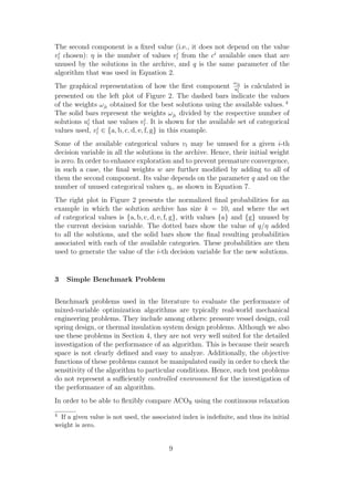
In order to be able to evaluate the objective function for a given TISD prob-
lem according to Equation 15, it is necessary to define several additional pa-
rameters. These are: the set of available materials, the thermodynamic cycle
efficiency coefficient at i-th intercept Ci , the effective thermal conductivity of
the insulator k for the available materials, the cross-section A, and the total
thickness L of the insulation.
Since both the cross-section and the total thickness have only linear influence
on the value of the objective function, we use normalized values A = 1 and L =
1 for simplicity. The thermodynamic cycle efficiency coefficient is a function
of the temperature, as follows:


 2.5



if T ≥ 71 K

C = 4 if 71 K > T > 4.2 K (17)




5 if T ≤ 4.2 K
The set of materials defined initially by Hilal and Boom [HB77], and later
also used by Kokkolaras et al. [KAD01] includes: teflon (T), nylon (N), epoxy-
fiberglass (in plane cloth) (F), epoxy-fiberglass (in normal cloth) (E), stainless
steel (S), aluminum (A), and low-carbon steel (L):
M = {T, N, F, E, S, A, L} (18)
26

29. The effective thermal conductivity k of all these insulators varies heavily with
the temperature and does so differently for different materials. Hence, which
material is better depends on the temperature and it is impossible to define a
temperature-independent ordering of the insulation effectiveness of the mate-
rials.
The tabulated data of the effective thermal conductivity k that we use in this
work comes from [Bar66]. Since ACOR is implemented in R, the tabulated data
has been fitted with cubic splines directly in R for the purpose of calculating
the integrals in the objective function given in Equation 15.
4.3.2 Experimental Setup
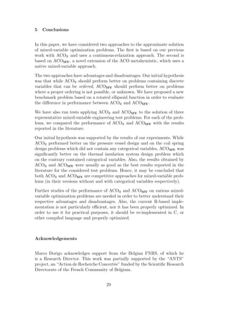
The constraints defined in Table 11 are met through the use of either a penalty
or a repair function. First, constraint g3 is met through normalizing the ∆x
values. The constraint g2 is met through the design choice of using ∆T as
a variable and ensuring that no ∆T may be negative. The latter is ensured
together with meeting the constraint g1 by checking if any ∆x of ∆T chosen is
negative. If it is, the objective function returns infinity as the solution quality.
The problem may be defined for a different number of intercepts. It has been
shown by Kokkolaras et al. [KAD01] that generally adding more intercepts
allows to obtain better results. However, due to practical reasons, too many
intercepts cannot be used in a real thermal insulation system. Hence, we de-
cided to limit ourselves to n = 10 intercepts in our experiments (that is, our
TISD instance has 3(n + 1) = 33 decision variables).
Further, in order to obtain results comparable to those reported in the litera-
ture, we set to 2,350 the maximum number of objective function evaluations
for our algorithms. In this way, the results obtained by ACOR can be compared
to those reported by Kokkolaras et al. [KAD01].
All the results reported were obtained using 100 independent runs of both
ACOR and ACOMV on each of the problem instance tackled.
4.3.3 Parameter Tuning
Similarly to the problems presented earlier, we have used the F-RACE method
to choose the parameters. The parameters chosen this way for both ACOR and
ACOMV are summarized in Table 12.
4.3.4 Results
Because of the experimental setup that we chose, the performance of ACOR
and ACOMV could only be compared to the results obtained using mixed-
27

30. Table 12
Summary of the parameters chosen for ACOR and ACOMV for the TISD problem.
Parameter Symbol ACOR ACOMV
number of ants m 2 2
speed of convergence ξ 0.8 0.9
locality of the search q 0.01 0.025
archive size k 50 50
Table 13
The results obtained by ACOR and ACOMV on the TISD problem using n = 10
intercepts (i.e., 33 decision variables) and 2,350 function evaluations, compared to
those reported in the literature.
MVP ACOR ACOMV
min 25.36336 27.91392 25.27676
median - 36.26266 26.79740
max - 198.90930 29.92718
variable programming (MVP) by Kokkolaras et al. [KAD01]. 7
The results obtained by ACOR and ACOMV , as well as the result of MVP
algorithm, are summarized in Table 13. As mentioned earlier, we followed
the experimental setup used by Kokkolaras et al. [KAD01] for one of their
experiments. We used the TISD problem instance with n = 10 intercepts (i.e.,
3(n + 1) = 33 decision variables) and only 2,350 function evaluations.
It may be observed that indeed, this time ACOMV significantly outperforms
ACOR . This clearly supports our initial hypothesis. Similarly to the initial
benchmark problem we used, also on the TISD problem containing categorical
variables, the native mixed-variable ACOMV approach outperforms ACOR .
Comparing ACOR and ACOMV performance to MVP is more complicate.
While we have done 100 independent runs of both ACOR and ACOMV , Kokko-
laras et al. reports only one single result. Also, Kokkolaras et al. used a Matlab
implementation to fit the tabulated data and compute the integrals required
to calculate the value of the objective function, while we used R. Further-
more, the MVP results for n = 10 intercepts were obtained with MVP using
additional information about the problem. Due to all these reasons, it is not
possible to compare very precisely the results obtained by ACOR and ACOMV
to those of MVP. However, it may be concluded that the best results obtained
by ACOMV and MVP under similar conditions are comparable.
7 A similarly defined problem was also tackled by Hilal and Boom [HB77], but they
only considered very simple cases.
28

31. 5 Conclusions
In this paper, we have considered two approaches to the approximate solution
of mixed-variable optimization problems. The first is based on our previous
work with ACOR and uses a continuous-relaxation approach. The second is
based on ACOMV , a novel extension of the ACO metaheuristic, which uses a
native mixed-variable approach.
The two approaches have advantages and disadvantages. Our initial hypothesis
was that while ACOR should perform better on problems containing discrete
variables that can be ordered, ACOMV should perform better on problems
where a proper ordering is not possible, or unknown. We have proposed a new
benchmark problem based on a rotated ellipsoid function in order to evaluate
the difference in performance between ACOR and ACOMV .
We have also run tests applying ACOR and ACOMV to the solution of three
representative mixed-variable engineering test problems. For each of the prob-
lems, we compared the performance of ACOR and ACOMV with the results
reported in the literature.
Our initial hypothesis was supported by the results of our experiments. While
ACOR performed better on the pressure vessel design and on the coil spring
design problems which did not contain any categorical variables, ACOMV was
significantly better on the thermal insulation system design problem which
on the contrary contained categorical variables. Also, the results obtained by
ACOR and ACOMV were usually as good as the best results reported in the
literature for the considered test problems. Hence, it may be concluded that
both ACOR and ACOMV are competitive approaches for mixed-variable prob-
lems (in their versions without and with categorical variables respectively).
Further studies of the performance of ACOR and ACOMV on various mixed-
variable optimization problems are needed in order to better understand their
respective advantages and disadvantages. Also, the current R-based imple-
mentation is not particularly efficient, nor it has been properly optimized. In
order to use it for practical purposes, it should be re-implemented in C, or
other compiled language and properly optimized.
Acknowledgements
Marco Dorigo acknowledges support from the Belgian FNRS, of which he
is a Research Director. This work was partially supported by the “ANTS”
project, an “Action de Recherche Concert´e” funded by the Scientific Research
e
Directorate of the French Community of Belgium.
29

32. References
[AD01] C. Audet and J.E. Dennis Jr. Pattern search algorithms for mixed
variable programming. SIAM Journal on Optimization, 11(3):573–594,
2001.
[Bar66] R. Barron. Cryogenic Systems. McGraw-Hill, New York, NY, 1966.
[Bir05] M. Birattari. The Problem of Tuning Metaheuristics as Seen from a
Machine Learning Perspective. PhD thesis, volume 292 of Dissertationen
zur K¨nstlichen Intelligenz.
u Akademische Verlagsgesellschaft Aka
GmbH, Berlin, Germany, 2005.
[BP95] G. Bilchev and I.C. Parmee. The ant colony metaphor for searching
continuous design spaces. In T. C. Fogarty, editor, Proceedings of the
AISB Workshop on Evolutionary Computation, volume 993 of LNCS,
pages 25–39. Springer-Verlag, Berlin, Germany, 1995.
[BSPV02] M. Birattari, T. St¨tzle, L. Paquete, and K. Varrentrapp. A racing
u
algorithm for configuring metaheuristics. In W. B. Langdon et al., editor,
Proceedings of the Genetic and Evolutionary Computation Conference,
pages 11–18. Morgan Kaufman, San Francisco, CA, 2002.
[CW97] Y.J. Cao and Q.H. Wu. Mechanical design optimization by mixed-
variable evolutionary programming. In Proceedings of the Fourth IEEE
Conference on Evolutionary Computation, pages 443–446. IEEE Press,
1997.
[DAGP90] J.-L. Deneubourg, S. Aron, S. Goss, and J.-M. Pasteels. The self-
organizing exploratory pattern of the Argentine ant. Journal of Insect
Behavior, 3:159–168, 1990.
[DG98] K. Deb and M. Goyal. A flexible optimiztion procedure for mechanical
component design based on genetic adaptive search. Journal of
Mechanical Design, 120(2):162–164, 1998.
[DMC96] M. Dorigo, V. Maniezzo, and A. Colorni. Ant System: Optimization by
a colony of cooperating agents. IEEE Transactions on Systems, Man,
and Cybernetics – Part B, 26(1):29–41, 1996.
[Dor92] M. Dorigo. Optimization, Learning and Natural Algorithms (in Italian).
PhD thesis, Dipartimento di Elettronica, Politecnico di Milano, Italy,
1992.
[DS02] J. Dr´o and P. Siarry. A new ant colony algorithm using the heterarchical
e
concept aimed at optimization of multiminima continuous functions. In
M. Dorigo, G. Di Caro, and M. Sampels, editors, Proceedings of the Third
International Workshop on Ant Algorithms (ANTS’2002), volume 2463
of LNCS, pages 216–221. Springer-Verlag, Berlin, Germany, 2002.
[DS04] M. Dorigo and T. St¨tzle.
u Ant Colony Optimization. MIT Press,
Cambridge, MA, 2004.
30

33. [FFC91] J.-F. Fu, R.G. Fenton, and W.L. Cleghorn. A mixed integer-discrete-
continuous programming method and its application to engineering
design optimization. Engineering Optimization, 17(4):263–280, 1991.
[GHYC04] C. Guo, J. Hu, B. Ye, and Y. Cao. Swarm intelligence for mixed-
variable design optimization. Journal of Zhejiang University SCIENCE,
5(7):851–860, 2004.
[GM02] M. Guntsch and M. Middendorf. A population based approach for ACO.
In S. Cagnoni, J. Gottlieb, E. Hart, M. Middendorf, and G. Raidl, editors,
Applications of Evolutionary Computing, Proceedings of EvoWorkshops
2002: EvoCOP, EvoIASP, EvoSTim, volume 2279 of LNCS, pages 71–80.
Springer-Verlag, Berlin, Germany, 2002.
[HB77] M.A. Hilal and R.W. Boom. Optmization of mechanical supports for
large super-conductive magnets. Advances in Cryogenic Engineering,
22:224–232, 1977.
[KAD01] M. Kokkolaras, C. Audet, and J.E. Dennis Jr. Mixed variable
optimization of the number and composition of heat intercepts in a
thermal insulation system. Optimization and Engineering, 2(1):5–29,
2001.
[LC94] H.-L. Li and C.-T. Chou. A global approach for nonlinear mixed discrete
programing in design optimization. Engineering Optimization, 22:109–
122, 1994.
[LLMB89] Q. Li, X. Li, G.E. McIntosh, and R.W. Boom. Minimization of total
refrigiration power of liquid neon and nitrogen cooled intercepts for
SMES magnets. Advances in Cryogenic Engineering, 35:833–840, 1989.
[LP91] H.T. Loh and P.Y. Papalambros. Computation implementation
and test of a sequential linearization approach for solving mixed-
discrete nonlinear design optimization. Journal of Mechanical Design,
113(3):335–345, 1991.
[LZ99a] J. Lampinen and I. Zelinka. Mechanical engineering design optimization
by differential evolution. In D. Corne, M. Dorigo, and F. Glover, editors,
New Ideas in Optimization, pages 127–146. McGraw-Hill, London, UK,
1999.
[LZ99b] J. Lampinen and I. Zelinka. Mixed integer-discrete-continuous
optimization by differential evolution, part 1: the optimization method.
In P. O˘mera, editor, Proceedigns of MENDEL’99, 5th International
s
Mendel Conference of Soft Computing, pages 71–76. Brno University
of Technology, Brno, Czech Repuplic, 1999.
[LZ99c] J. Lampinen and I. Zelinka. Mixed integer-discrete-continuous
optimization by differential evolution, part 2: a practical example.
In P. O˘mera, editor, Proceedigns of MENDEL’99, 5th International
s
Mendel Conference of Soft Computing, pages 77–81. Brno University
of Technology, Brno, Czech Repuplic, 1999.
31

34. [MHM89] Z. Musicki, M.A. Hilal, and G.E. McIntosh. Optimization of cryogenic
and heat removal system of space borne magnets. Advances in Cryogenic
Engineering, 35:975–982, 1989.
[MVS00] N. Monmarch´, G. Venturini, and M. Slimane. On how Pachycondyla
e
apicalis ants suggest a new search algorithm. Future Generation
Computer Systems, 16:937–946, 2000.
[OS02] J. Oˇen´ˇek and J. Schwarz. Estimation distribution algorithm for
c as
mixed continuous-discrete optimization problems. In Proceedings of the
2nd Euro-International Symposium on Computational Intelligence, pages
227–232. IOS Press, Amsterdam, Netherlands, 2002.
[PA92] S. Praharaj and S. Azarm. Two level nonlinear mixed discrete continuous
optimization-based design: An application to printed circuit board
assemblies. Journal of Electronic Packaging, 114(4):425–435, 1992.
[PK05] R. Pandia Raj and V. Kalyanaraman. GA based optimal design of steel
truss bridge. In J. Herskovits, S. Mazorche, and A. Canelas, editors,
Proceedigns of 6th World Congress of Structural and Multidisciplinary
Optimization, pages CD–ROM proceedings, 2005.
[San90] E. Sandgren. Nonlinear integer and discrete programming in mechanical
design optimization. Journal of Mechanical Design, 112:223–229, 1990.
[SB97] M.A. Stelmack and S.M. Batill. Concurrent subspace optimization of
mixed continuous/discrete systems. In Proceedings
of AIAA/ASME/ASCE/AHS/ASC 38th Structures, Structural Dynamic
and Materials Conference. AIAA, Reston, VA, 1997.
[SBR94] R.S. Sellar, S.M. Batill, and J.E. Renaud. Optimization of
mixed discrete/continuous design variable systems using neural
networks. In Proceedings of AIAA/USAF/NASA/ISSMO Symposium on
Multidisciplinary Analysis and Optimization. AIAA, Reston, VA, 1994.
[SD06] K. Socha and M. Dorigo. Ant colony optimization for
continuous domains. European Journal of Operational Research, page
doi:10.1016/j.ejor.2006.06.046, 2006.
[Soc04] K. Socha. ACO for continuous and mixed-variable optimization. In
M. Dorigo, M. Birattari, C. Blum, L. M. Gambardella, F. Mondada, and
T. St¨tzle, editors, Ant Colony Optimization and Swarm Intelligence,
u
4th International Workshop, ANTS 2004, volume 3172 of LNCS, pages
25–36. Springer-Verlag, Berlin, Germany, 2004.
[ST05] H. Schmidt and G. Thierauf. A combined heuristic optimization
technique. Advances in Engineering Software, 36:11–19, 2005.
[TC00] G. Thierauf and J. Cai. Evolution strategies—parallelization and
application in engineering optimization. In B.H.V. Topping, editor,
Parallel and distributed processing for computational mechanics: systems
and tools, pages 329–349. Saxe-Coburg Publications, Edinburgh, UK,
2000.
32

35. [Tur03] N. Turkkan. Discrete optimization of structures using a floating point
genetic algorithm. In Proceedings of Annual Conference of the Canadian
Society for Civil Engineering, pages CD–ROM proceedings, 2003.
[WC95] S.-J. Wu and P.-T. Chow. Genetic algorithms for nonlinear mixed
discrete-integer optimization problems via meta-genetic parameter
optimization. Engineering Optimization, 24(2):137–159, 1995.
[YOY91] M. Yamaguchi, T. Ohmori, and A. Yamamoto. Design optimization of
a vapor-cooled radiation shield for LHe cryostat in space use. Advances
in Cryogenic Engineering, 37:1367–1375, 1991.
33