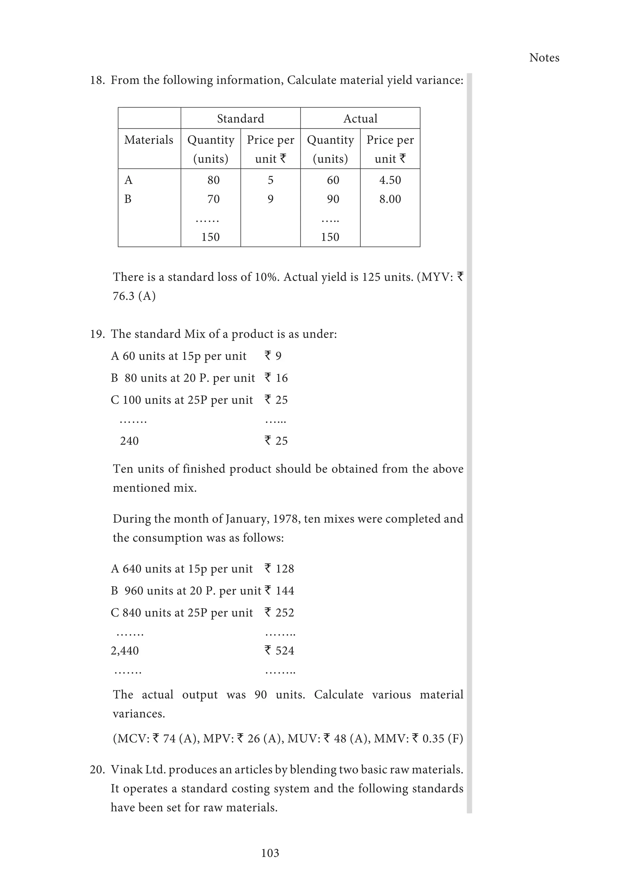
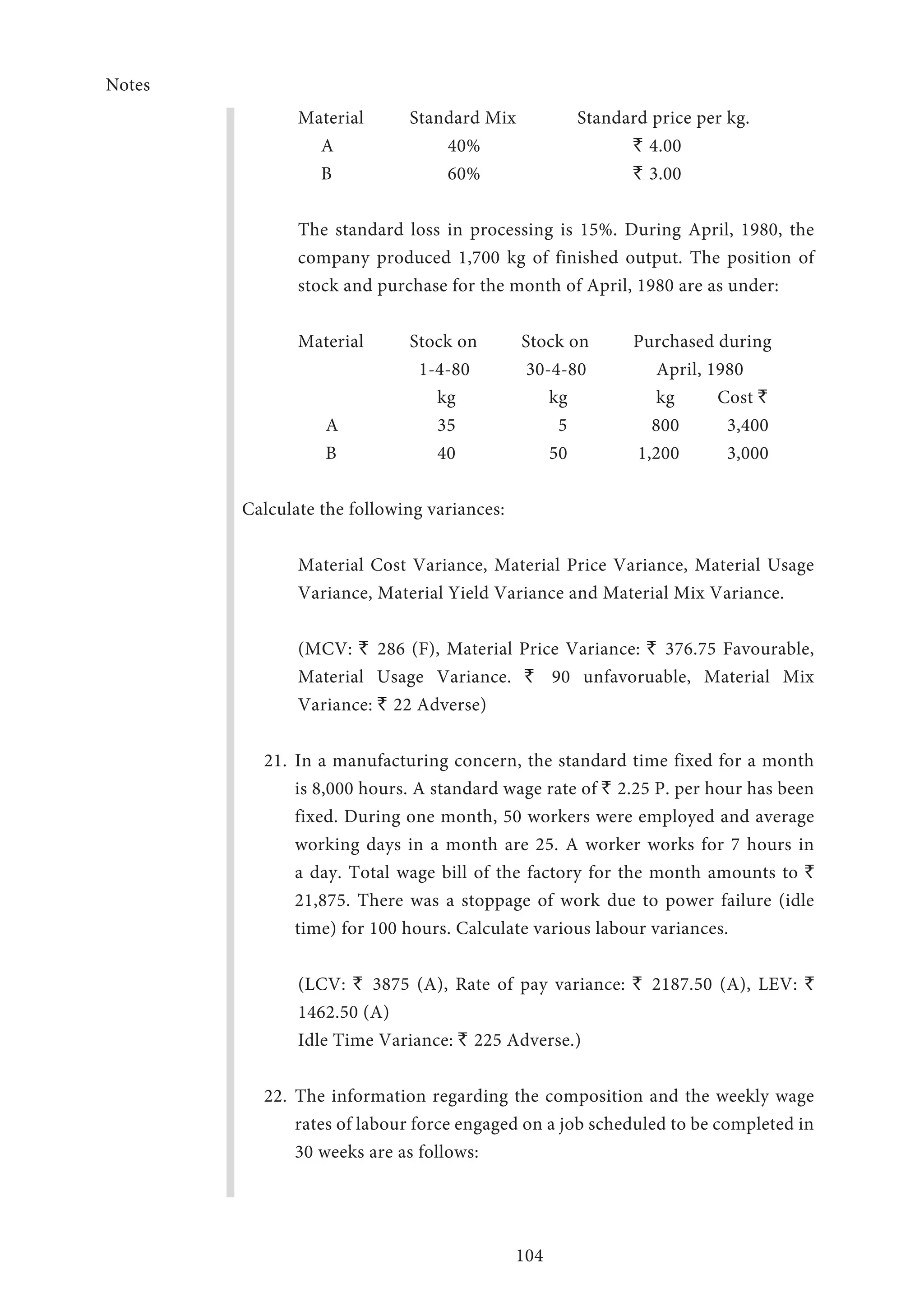
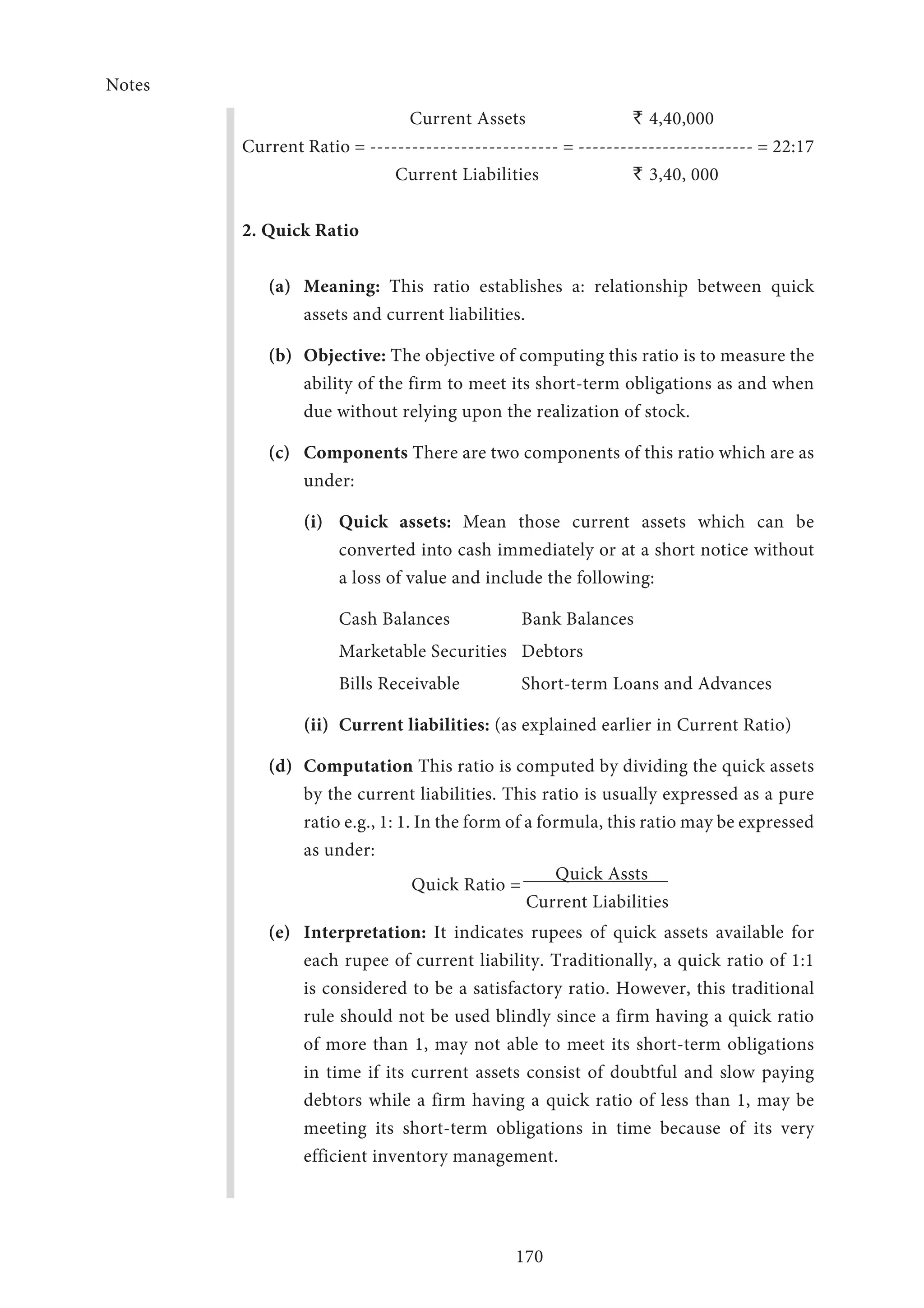
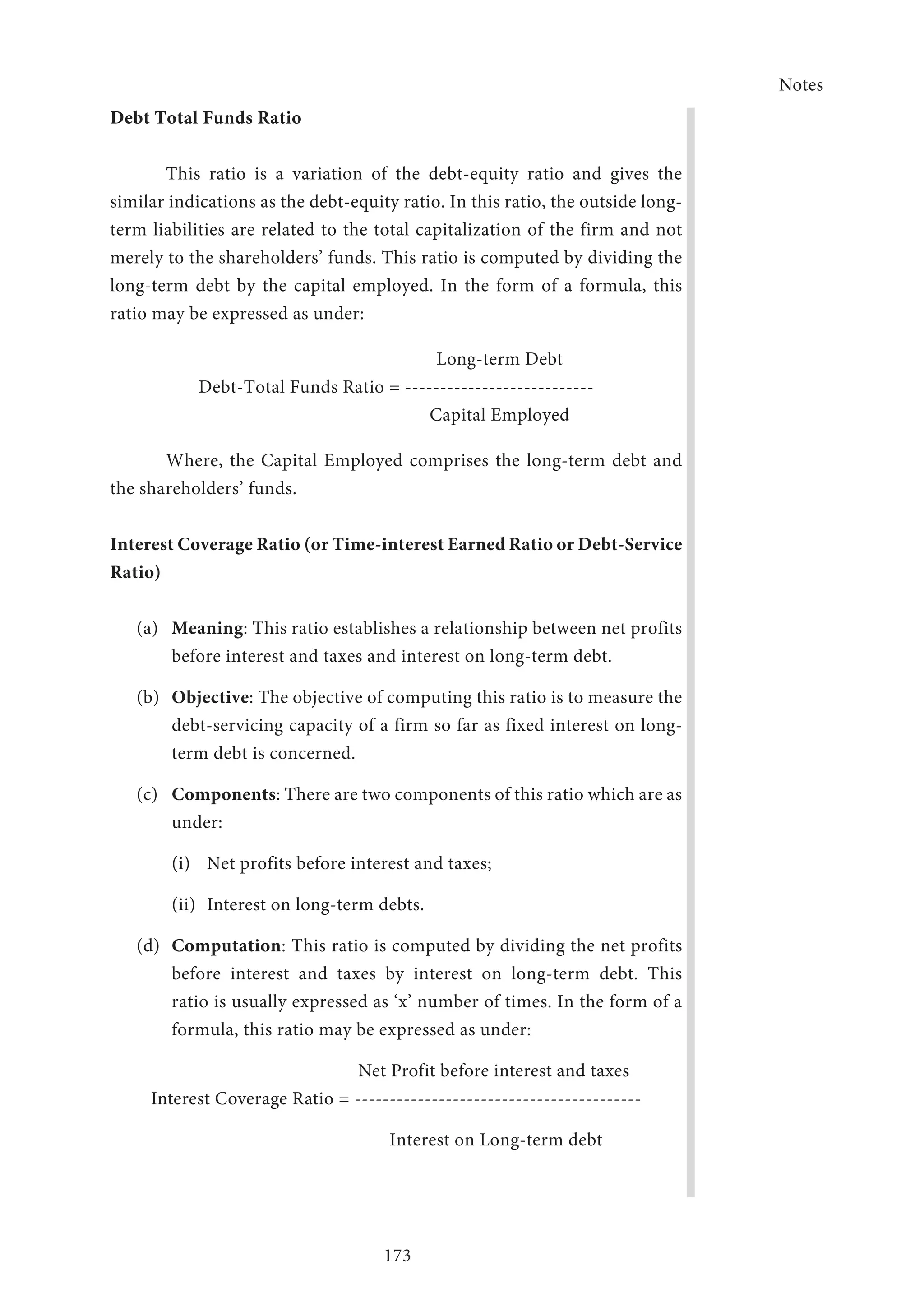
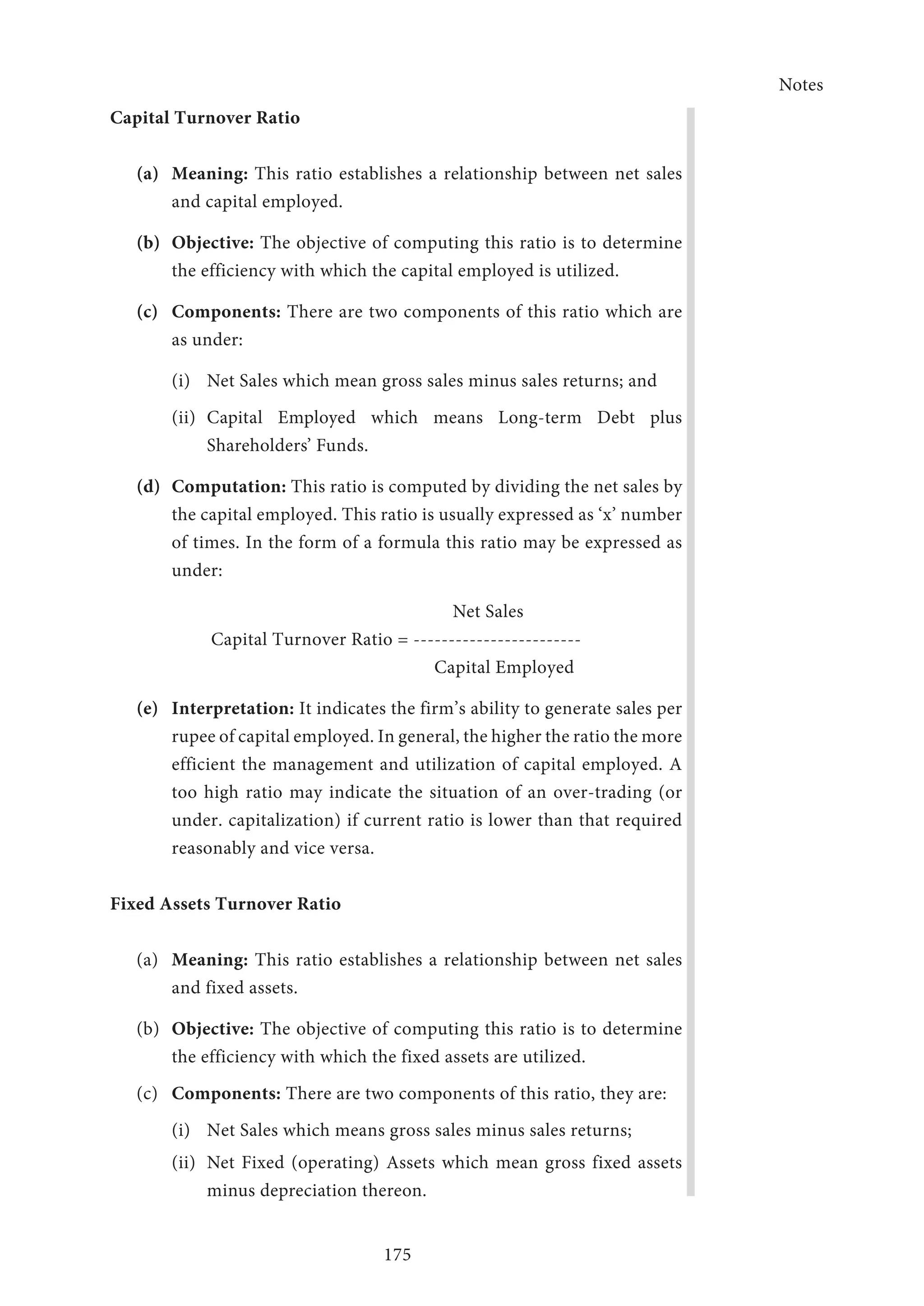
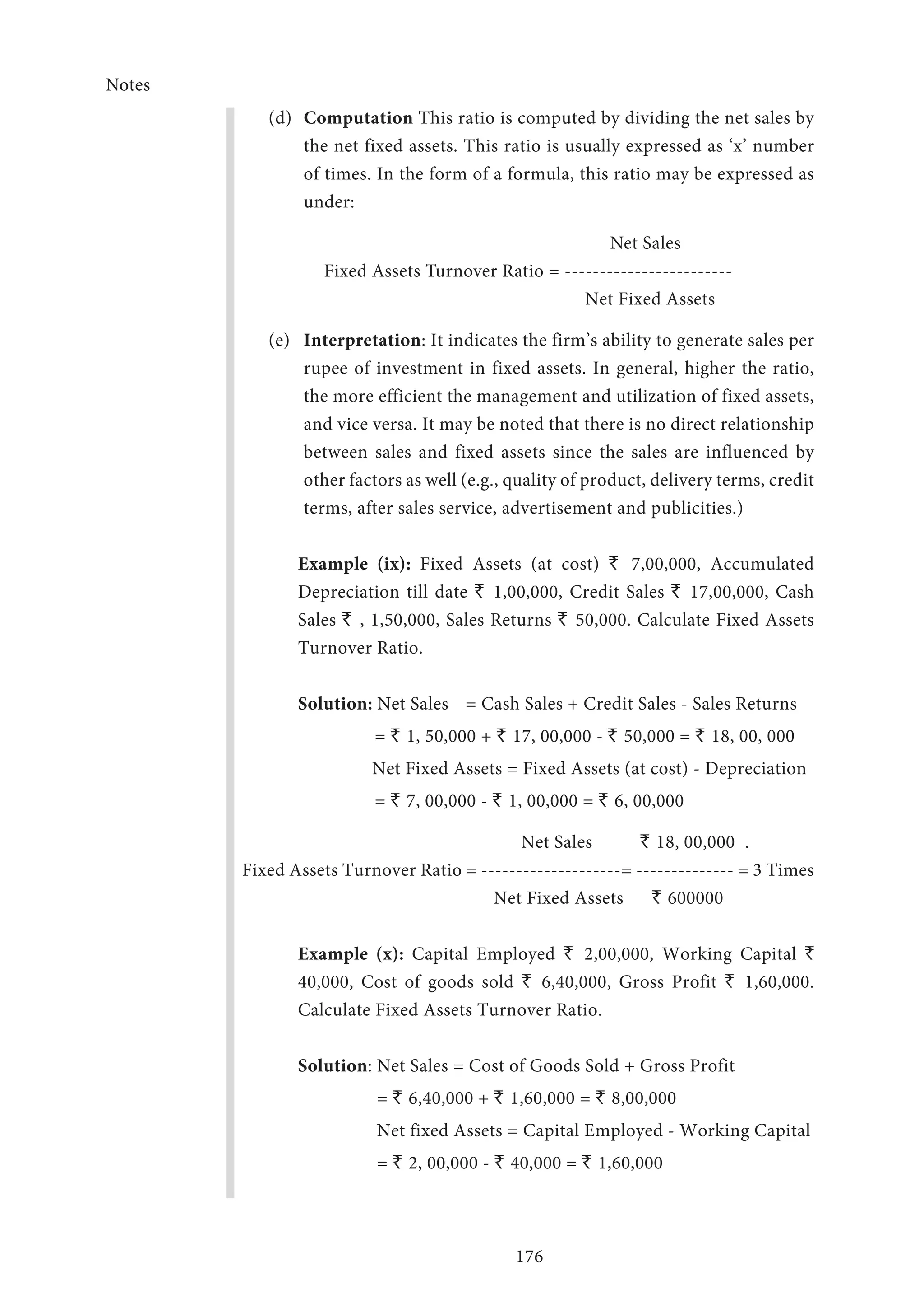
Download to read offline


![Notes
2
Unit – III
Marginal Costing and Break-even Analysis – Cost-Volume-Profit
(CVP) Analysis – Break-Even Analysis – Assumptions and practical
applications of Breakeven-Analysis – Decisions regarding Sales-mix –
Make or Buy Decisions – Limiting Factor Decision – Export Decision –
Plant Merger – Decision of Shutdown or Continuation of a product line.
Unit - IV
DuPont Analysis – Fund Flow Analysis – Cash flow analysis –
Contemporary Issues in Management Accounting – Value chain analysis
– Activity-Based Costing (ABC) – Quality Costing – Target and Life Cycle
Costing – Theory of Constraints accounting (TOC).
Unit – V
Social Cost Benefit Analysis – Decision Tree in Management –
Reporting to Management – Objectives of Reporting – Reporting needs
at different managerial levels – Types of reports – Modes of Reporting,
Reporting at different levels of Management.
[Note: Distribution of Questions between Problems and Theory
of this paper must be 60:40 i.e., Problem Questions: 60 % & Theory
Questions: 40%]
References
Dr Murthy, S Gurusamy, MANAGEMENT ACCOUNTING, McGraw
Hill, Delhi, 2009
Khan. MY, Jain P., MANAGEMENT ACCOUNTING, McGraw Hill, Delhi,
2009
Singhvi. NM, MANAGEMENT ACCOUNTING, PHI, Delhi, 2010](https://image.slidesharecdn.com/accountingmanagement230813-200304093208/75/Accounting-management230813-6-2048.jpg)


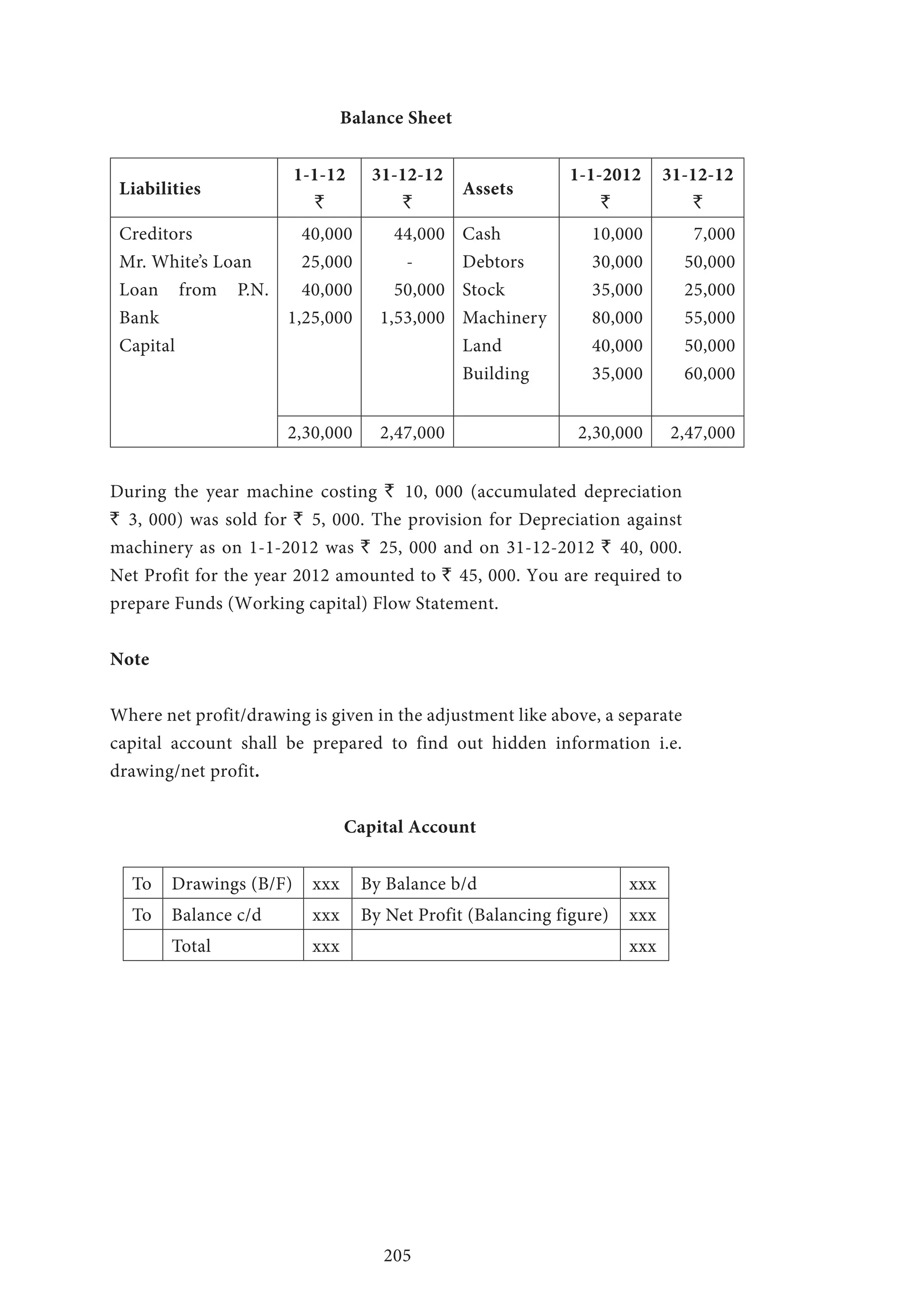


This document provides an overview of management accounting. It defines accounting as the process of recording, classifying, summarizing, analyzing and interpreting financial transactions of a business. It then discusses the three branches of accounting: financial accounting, cost accounting, and management accounting. Financial accounting is concerned with preparing financial statements to ascertain results and financial position. However, financial accounting has limitations and does not provide all the information managers need for planning, decision making, and control. Management accounting aims to address these limitations.


