Download to read offline


![ie e viene descritta dalla birth-deah master equation [8], che descrive la probabilità P(n, t)
data specie al tempo t di avere una popolazione di n individui
dP
dt
(n, t) = b(n 1) · P(n 1, t) [b(n) + d(n)] · P(n, t) + d(n + 1) · P(n + 1, t)
e b(n) e d(n) sono rispettivamente i parametri di nascita e morte, dati dalle seguenti
b(n) = (1 n) ·
n
J
J n
J 1
d(n) = (1 n) ·
n
J
J n
J 1
+ n ·
n
J
Notiamo che queste definizioni sono consistenti con le due regole della dinamica del V
del:
con probabilità 1 n si ha la morte di un individuo della comunità non appartenente
specie data (con probabilità J n
J ) accompagnata dalla nascita di un individuo della sp
scelta ( n
J 1 );
con probabiltà n
J si ha la morte di un individuo appartenente alla specie data accompag
ta o dalla migrazione di un individuo proveniente da una delle altre specie presenti
probabilità (1 n)
⇣
J n
J 1
⌘
) o dalla comparsa di una nuova specie (con probabilità n).
oluzione stazionaria o di equilibrio P⇤(n) per la (3.1) è la seguente [8]
escritta dalla birth-deah master equation [8], che descrive la probabilità P(n, t) per
al tempo t di avere una popolazione di n individui
) = b(n 1) · P(n 1, t) [b(n) + d(n)] · P(n, t) + d(n + 1) · P(n + 1, t) (3.1)
) sono rispettivamente i parametri di nascita e morte, dati dalle seguenti
b(n) = (1 n) ·
n
J
J n
J 1
(3.2)
d(n) = (1 n) ·
n
J
J n
J 1
+ n ·
n
J
(3.3)
e queste definizioni sono consistenti con le due regole della dinamica del Voter
bilità 1 n si ha la morte di un individuo della comunità non appartenente alla
a (con probabilità J n
J ) accompagnata dalla nascita di un individuo della specie
);
biltà n
J si ha la morte di un individuo appartenente alla specie data accompagna-
migrazione di un individuo proveniente da una delle altre specie presenti (con
à (1 n)
⇣
J n
J 1
⌘
) o dalla comparsa di una nuova specie (con probabilità n).
zionaria o di equilibrio P⇤(n) per la (3.1) è la seguente [8]
Ciascun nodo è un individuo rappresentato da un label che ne identifi
za. Denotiamo con C la collezione di tutti gli individui appartenenti a
~n = {n1, n2, . . . , nS} il vettore delle abbondanze per C, dove nj indica
della j-esima specie.
Ci poniamo nell’ensemble microcanonico, imponendo che ogni in
sostituito immediatamente da un altro della stessa o di un’altra specie
J =
S
Â
i=1
ni
La dinamica del mean field Voter Model a ogni istante di tempo è
selezionato casualmente muore e viene sostituito con un individuo di
probabilità n, mentre con probabilità 1 n il sito viene colonizzato d
presente su un nodo selezionato casualmente nella griglia. A differe
del Voter Model, dove l’interazione avveniva tra primi vicini, nel mode
con qualsiasi nodo della griglia, senza che però ci sia dispersione sulla
Il parametro n, detto diversification rate, gioca un ruolo fondamental
da che esso sia o meno nullo, la dinamica è completamente differente
parla di mean field Voter Model senza speciazione e in questo caso s
specie: in un tempo finito tutti i nodi saranno occupati da individui
popolazione dei votanti ha raggiunto un consenso). Se, invece, n > 0
Model con speciazione: in questo caso, in un tempo finito si raggiun
della distribuzione delle specie presenti.
P⇤
(n) = P(0)
n
’
z=1
b(z 1)
d(z)
(3.4)
e dedotta dalla condizione di normalizzazione
Â
n
P⇤
(n) = 1
esto risultato, imponiamo la condizione di equilibrio dP
dt (n, t) = 0 e notiamo
ere l’equazione come
I(n + 1) I(n) = 0 (3.5)
to
I(n) = d(n)P⇤
(n) b(n 1)P⇤
(n 1)
zione fisica che non si possa avere un numero di individui negativo, si ha che
quindi, I(0) = 0. Inoltre, supporre che quando una specie si estingue con-
na nuova la rimpiazza è equivalente a imporre condizioni al contorno riflet-
a ipotesi è ragionevole sulle scale temporali di nostro interesse. Sommando
otteniamo
1
[I(z + 1) I(z)] = I(n) I(0) = 0 =) I(n) = 0
La soluzione stazionaria o di equilibrio P⇤(n) per la (3.1) è la segue
P⇤
(n) = P(0)
n
’
z=1
b(z 1)
d(z)
dove P(0) può essere dedotta dalla condizione di normalizzazione
Â
n
P⇤
(n) = 1
Per arrivare a questo risultato, imponiamo la condizione di equ
che possiamo riscrivere l’equazione come
I(n + 1) I(n) = 0
dove abbiamo definito
I(n) = d(n)P⇤
(n) b(n 1)P⇤
(n 1
Imponendo la condizione fisica che non si possa avere un numero d
b( 1) = d(0) = 0 e, quindi, I(0) = 0. Inoltre, supporre che quan
temporaneamente una nuova la rimpiazza è equivalente a imporr
tenti alla (3.1): questa ipotesi è ragionevole sulle scale temporali d
Per arrivare a questo ri
che possiamo riscrivere l’e
dove abbiamo definito
Imponendo la condizione
b( 1) = d(0) = 0 e, quin
temporaneamente una nu
tenti alla (3.1): questa ipot
su tutti gli n la (3.5) ottenia
n 1
Â
z=0
[I(z +
da cui segue che P⇤(n) è ri
z=1
dove P(0) può essere dedotta dalla condizione di normali
Â
n
P⇤
(n) = 1
Per arrivare a questo risultato, imponiamo la condizio
che possiamo riscrivere l’equazione come
I(n + 1) I(n) = 0
dove abbiamo definito
I(n) = d(n)P⇤
(n) b(n 1)
Imponendo la condizione fisica che non si possa avere un
b( 1) = d(0) = 0 e, quindi, I(0) = 0. Inoltre, supporre c
temporaneamente una nuova la rimpiazza è equivalente
tenti alla (3.1): questa ipotesi è ragionevole sulle scale tem
su tutti gli n la (3.5) otteniamo
n 1
Â
z=0
[I(z + 1) I(z)] = I(n) I(0) = 0
e P(0) può essere dedotta dalla condizione di normalizzazione
Â
n
P⇤
(n) = 1
Per arrivare a questo risultato, imponiamo la condizione di equilibrio dP
dt (n, t) = 0 e notiamo
possiamo riscrivere l’equazione come
I(n + 1) I(n) = 0 (3.5
e abbiamo definito
I(n) = d(n)P⇤
(n) b(n 1)P⇤
(n 1)
onendo la condizione fisica che non si possa avere un numero di individui negativo, si ha che
1) = d(0) = 0 e, quindi, I(0) = 0. Inoltre, supporre che quando una specie si estingue con
poraneamente una nuova la rimpiazza è equivalente a imporre condizioni al contorno riflet
i alla (3.1): questa ipotesi è ragionevole sulle scale temporali di nostro interesse. Sommando
utti gli n la (3.5) otteniamo
n 1
Â
z=0
[I(z + 1) I(z)] = I(n) I(0) = 0 =) I(n) = 0
ui segue che P⇤(n) è ricorsiva, come si voleva: d(n)P⇤(n) = b(n 1)P⇤(n 1).
Â
n
P⇤
(n) = 1
niamo la condizione di equilibrio dP
dt (n, t) = 0 e notiamo
e
n + 1) I(n) = 0 (3.5)
)P⇤
(n) b(n 1)P⇤
(n 1)
si possa avere un numero di individui negativo, si ha che
noltre, supporre che quando una specie si estingue con-
za è equivalente a imporre condizioni al contorno riflet-
ole sulle scale temporali di nostro interesse. Sommando
I(n) I(0) = 0 =) I(n) = 0
si voleva: d(n)P⇤(n) = b(n 1)P⇤(n 1).
dP
dt
(n, t) = b(n 1) · P(n 1, t) [b(n) + d(n)] · P(n, t) + d(n + 1) ·
dove b(n) e d(n) sono rispettivamente i parametri di nascita e morte, dati dal
b(n) = (1 n) ·
n
J
J n
J 1
d(n) = (1 n) ·
n
J
J n
J 1
+ n ·
n
J
Notiamo che queste definizioni sono consistenti con le due regole della
Model:
• con probabilità 1 n si ha la morte di un individuo della comunità no
specie data (con probabilità J n
J ) accompagnata dalla nascita di un ind
scelta ( n
J 1 );
• con probabiltà n
J si ha la morte di un individuo appartenente alla specie
ta o dalla migrazione di un individuo proveniente da una delle altre s
probabilità (1 n)
⇣
J n
J 1
⌘
) o dalla comparsa di una nuova specie (con p
La soluzione stazionaria o di equilibrio P⇤(n) per la (3.1) è la seguente [8]
P⇤
(n) = P(0)
n
’
z=1
b(z 1)
d(z)
dove P(0) può essere dedotta dalla condizione di normalizzazione
Mapping birth-death ME with Voter Model: Analytical Solution
Birth rate
Death rate
BCCurrent of probability
Solution](https://image.slidesharecdn.com/udinesummerschool-suweis-180909213937/75/A-statistical-physics-approach-to-system-biology-27-2048.jpg)


![Connected components in a network
Laplacian matrix!
The Laplacian matrix is a similarly useful matrix defined by:!
L = K - A!
dΨ[t]/dt=-DLΨ[t]
Eigenvalues of L
Connected Compone](https://image.slidesharecdn.com/udinesummerschool-suweis-180909213937/75/A-statistical-physics-approach-to-system-biology-39-2048.jpg)

![y health
of com-
m patho-
nt (3–6).
s ecolog-
different
tends to
periods
for host
res that
unctions
espond-
ity com-
h (4, 13).
en char-
al work.
erstand-
rticular,
y. There
heory to
erns for
n made
dels (14)
ities (15).
y diverse
), which
llenging
ecology
dels that
rge and
develop
he gen-
where the types of interactions between species
are randomly distributed, meaning that +/+ (coop-
eration) and –/– (competition) interactions occur
with half the probability of +/– (exploitation) inter-
actions. Also, whereas ecological competition is
thought to be prevalent in natural microbial com-
munities (20), it is commonly assumed that the
functioning of microbiome communities restsupon
species that engage in cooperative metabolism (+/+)
potentialcommunitytypes,coveringthefullrangeof
possible interactions and species diversities [Fig. 1
and supplementary method 1 (31)]. We develop
our theory for unstructured ecological networks
because, unlike in plant-pollinator communities
or food webs (32, 33), there is no evidence of strong
structuring within microbial communities (16).
However, although no single structure type dom-
inates in these communities, our mathematics
Fig. 1. Ecological theory and microbiota stability. (A) Ecological network theory captures networks of
microbial species that interact with themselves (–s) and other genotypes (aij). (B) Coupled ordinary differential
onNovemwww.sciencemag.orgDownloadedfromonNovemwww.sciencemag.orgDownloadedfromonNovemwww.sciencemag.orgDownloadedfromonNovemwww.sciencemag.orgDownloadedfrom
tion of cooperative interactions within communi-
ties nearly always decreases the overall return
rate and the likelihood of stability [Fig. 2 and
lysis, we find the same
is destabilizing. Howe
plementary materials
Fig. 2. Cooperation reduces community stability. (A) Illustration of changin
the proportion of cooperative links in networks. Pm, proportion of cooperative in
MICROBIOME
The ecology of the microbiome:
Networks, competition, and stability
Katharine Z. Coyte,1,2
* Jonas Schluter,1,2,3
*† Kevin R. Foster1,2
†
The human gut harbors a large and complex community of beneficial microbes that remain stable
over long periods.This stability is considered critical for good health but is poorly understood.
Here we develop a body of ecological theory to help us understand microbiome stability.
Although cooperating networks of microbes can be efficient, we find that they are often unstable.
Counterintuitively, this finding indicates that hosts can benefit from microbial competition when
this competition dampens cooperative networks and increases stability. More generally, stability is
promoted by limiting positive feedbacks and weakening ecological interactions.We have analyzed
host mechanisms for maintaining stability—including immune suppression, spatial structuring, and
feeding of community members—and support our key predictions with recent data.
T
he human microbiome contains hundreds
of species and trillions of cells that reside
predominantly in the gastrointestinal tract
(1, 2). These microbes provide many health
benefits, including the breakdown of com-
plex molecules in food, protection from patho-
gens, and healthy immune development (3–6).
The gut microbiome is often noted for its ecolog-
ical stability. Different people may carry different
microbial species, but any one individual tends to
carry the same key set of species for long periods
(6–8). This stability is considered critical for host
Seminal work by May suggests that species di-
versity can be problematic for community stability
(17, 19). However, May’s work focused on networks
where the types of interactions between species
are randomly distributed, meaning that +/+ (coop-
eration) and –/– (competition) interactions occur
with half the probability of +/– (exploitation) inter-
actions. Also, whereas ecological competition is
thought to be prevalent in natural microbial com-
munities (20), it is commonly assumed that the
functioning of microbiome communities restsupon
species that engage in cooperative metabolism (+/+)
and
The
Com
num
tera
anti
coop
prod
ly re
olism
alth
tent
ecol
T
biom
fects
with
crob
ics. T
of th
subs
gene
pote
poss
and
our
beca
or fo
stru
How
inat](https://image.slidesharecdn.com/udinesummerschool-suweis-180909213937/75/A-statistical-physics-approach-to-system-biology-42-2048.jpg)


![Why do physicists care ?
PPLEMENTARY INFORMATION
50 100 200 500
0.02
0.05
0.10
0.20
0.50
Number of Species [S]
Connectance[CΓ
]
C~1/S](https://image.slidesharecdn.com/udinesummerschool-suweis-180909213937/75/A-statistical-physics-approach-to-system-biology-50-2048.jpg)


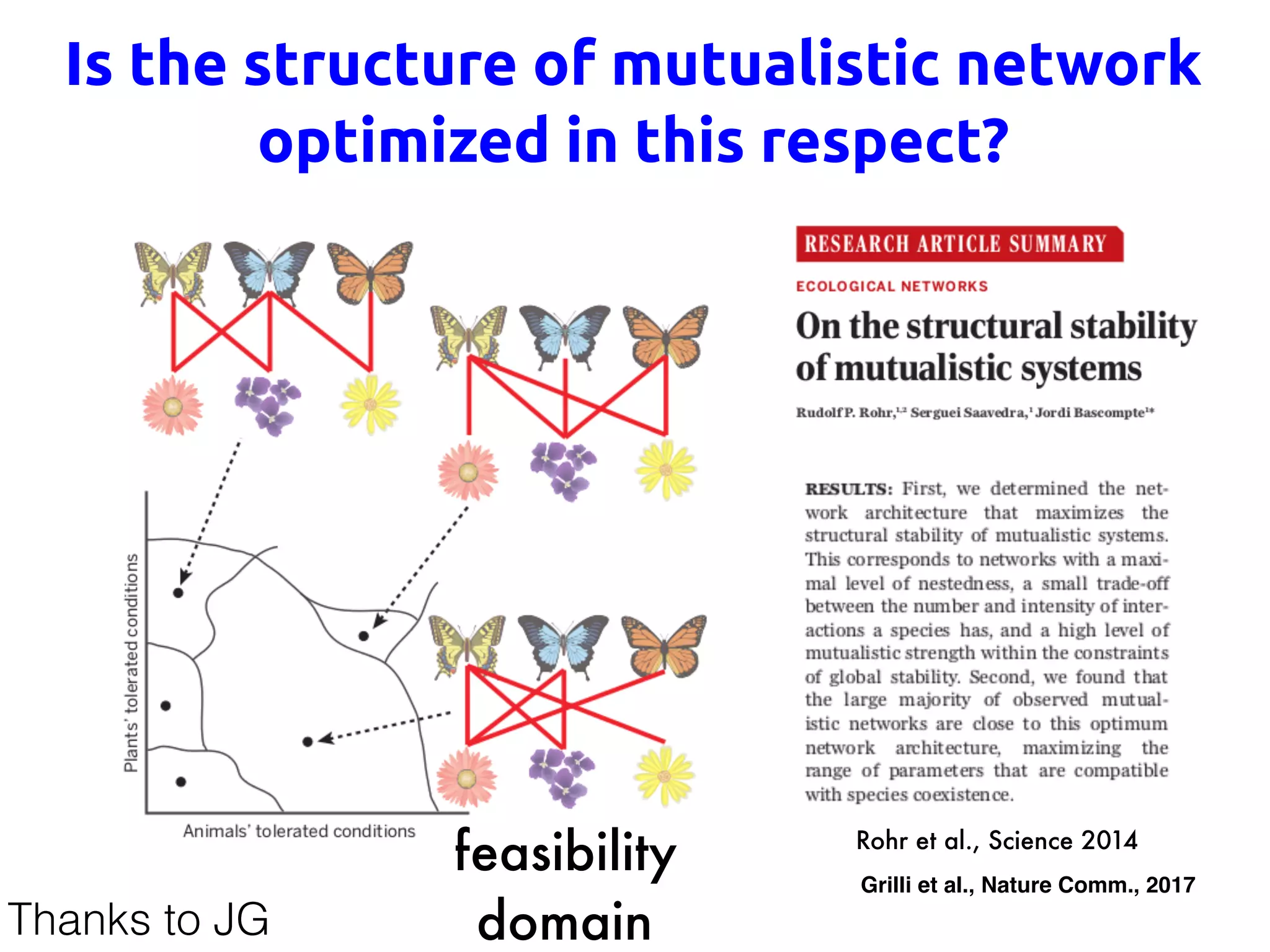
![Why this recurrent topological properties?
Optimization Principles to explain
emergent patterns
UPPLEMENTARY INFORMATION
50 100 200 500
0.02
0.05
0.10
0.20
0.50
Number of Species [S]
Connectance[CΓ
]
e S1: Best fit (red solid line) of the connectivity as a function of the number of
es for 56 mutualistic communities. Dashed gray lines represent the region within
±1 standard deviation confidence interval for the exponent estimate. The plot is in
g scale.
C~1/S
Busiello et al., Scientific Report
The Origin of Sparsity in the Interaction Networks of Living Systems
This talk](https://image.slidesharecdn.com/udinesummerschool-suweis-180909213937/75/A-statistical-physics-approach-to-system-biology-54-2048.jpg)

![Network data vs Randomization 1
Null model 1: we keep fixed S and C,
and place at random the edges
# Species [S]
Nestedness[NODF]
20 40 60 80 100 120 140 160 180 200
0
0.1
0.2
0.3
0.4
0.5
0.6
0.7
0.8
Random
Data](https://image.slidesharecdn.com/udinesummerschool-suweis-180909213937/75/A-statistical-physics-approach-to-system-biology-57-2048.jpg)


![Relation between sigle species and total abundance
i
li
j
|γij
|=0.0017
|γij
|=0
T=n
i
li
j
|γij
|=0.0017
|γij
|=0
T=n+1
swap
0.803522
1.08178
1.05803
1.05014
0.977939
1.01422
0.958128
1.13397
1.04078
1.0356
0.9664
1.02013
1.00682
0.67361
1.10131
1.07571
1.10289
0.959658
0.996913
0.918892
1.15298
1.03813
1.0223
1.01314
0.958794
1.00217
::
x* = x* =
T T+1
i j
l
k j
l
swap
δWilMil
x⇤
= M 1
· ↵
���� �����
����������[��]
Suweis et al., Nature 2013](https://image.slidesharecdn.com/udinesummerschool-suweis-180909213937/75/A-statistical-physics-approach-to-system-biology-72-2048.jpg)
![Overlap and community abundance are correlated!
M = M0 + V =
I + ⌦ O
O I + ⌦
+
O
T
O
xtot
= K + Co ) o / C 1
xtot
+ constant
0.2 0.3 0.4 0.5 0.6 0.7 0.8
50
54
58
62
66
Nestedness [NODF]
Abundance[x]
C
ij =
⇢
with probability C ( > 0)
0 with probability 1 C
⌦ij = C!(1 ij) ! > 0
x⇤
= M 1
· ↵
Suweis et al., Nature 2013
x⇤
= M 1
· ↵ x⇤
+ x⇤
= (M + M) 1
· ↵
0 200 400 600 800 100012001400160018002000
9.8
10
10.2
10.4
10.6
10.8
11
11.2
11.4
11.6
11.8
STEPS [T]
Population
0 200 400 600 800 100012001400160018002000
9.8
10
10.2
10.4
10.6
10.8
11
11.2
11.4
11.6
11.8
STEPS [T]
Population
Averaged over 100 realizations
0 200 400 600 800 100012001400160018002000
19.5
20
20.5
21
21.5
22
22.5
STEPS [T]
TotoalPopulation
mean
1 realiz
if x⇤
k > 0 ) x⇤
tot > 0
Cooperation in nested mutualistic community!](https://image.slidesharecdn.com/udinesummerschool-suweis-180909213937/75/A-statistical-physics-approach-to-system-biology-73-2048.jpg)
![# Species [S]
Nestedness[NODF]
σΓ
=0.0025
σΓ
=0.05
20 40 60 80 100 120 140 160 180 200
0
0.1
0.2
0.3
0.4
0.5
0.6
0.7
0.8
Random σΓ
=0.025
DataA
Suweis et al., Nature 2013](https://image.slidesharecdn.com/udinesummerschool-suweis-180909213937/75/A-statistical-physics-approach-to-system-biology-74-2048.jpg)
![No! Optimal networks are less resilient
c
−0.05 −0.04 −0.03 −0.02 −0.01 0
0
0.01
0.02
0.03
0.04
0.05
Max[Re(λ)]RarestSpecies[x]
b
R2
=0.999
0 5 10 15 20 25
0
1
2
3
4
5
number of connections [k]
speciesabundance‹x›
si
=|∑j
γij
|
a
‹x›
pdf
Max[Re(λ)]
0 1 2
5
0
4
3
2
1
-0.8 -0.7 -0.6 -0.5 -0.4 -0.3
5
10
15
20
25
Suweis et al., Nature 2013
A CB
time
perturbationstrength
λH reactivity
λ1 resilience
amplitude1
d x
dt
= J x
Jv1 = 1v1
u1J = 1u1
Suweis et al., in Nature Communications 2015
Beyond Resilience: Localization](https://image.slidesharecdn.com/udinesummerschool-suweis-180909213937/75/A-statistical-physics-approach-to-system-biology-76-2048.jpg)


![0 200 400 600 800
1
2
5
10
20
50
Size S
rIPRleft
0 200 400 600 800
1.0
10.0
5.0
2.0
3.0
1.5
15.0
7.0
Size S
rIPRright
A B
Ecological networks are localized!
A1 = |⇠0|(
X
j
v1,j|)2
Localization attenuates perturbations
Max|{v1}
A1 = 1/
p
S
Min|{v1}
A1 = i,j⇤
●
●●
●
●
●
●
●
●●
●
●
●
●
●
●
●
●
●●
●
●
●
●
●
●
●
●
●
●
●
●
●
●●
●
●
●
●
●●
●
●
●
●
●
●
●
●
●
●
●
●●
●
●
●
●
●
■
■■
■
■
■
■
■
■■
■
■
■
■
■
■
■
■
■■
■
■
■■
■
■
■
■
■
■
■
■
■ ■■
■
■
■
■
■■
■
■
■
■
■
■
■
■
■
■
■
■
■
■
■
■
■
■
◆
◆
◆
◆◆
◆
◆
◆
◆
◆
◆
◆
◆
◆
◆
◆◆◆
◆◆
◆
◆
◆◆
◆
◆
◆
◆ ◆
◆
◆
◆
◆
◆
◆
◆
◆
◆
◆
◆◆
◆
◆
◆
◆
◆
◆
◆◆
◆
◆
◆
◆
◆◆
◆
◆
◆
◆
� ��� ��� ��� ���
���
���
���
���
���
���
���
���
���� [�]
/���
Trade Off with May!
Suweis et al., in Nature Communications 2015](https://image.slidesharecdn.com/udinesummerschool-suweis-180909213937/75/A-statistical-physics-approach-to-system-biology-80-2048.jpg)
![Localization occurs on the hubs
Suweis et al., in Nature Communications 2015
1.0
0.8
0.6
0.4
0.2
0 20 40 60
max=–0.27v1
u1
WH
s
smax
H=0.47
Species
TURE COMMUNICATIONS | DOI: 10.1038/ncomms10179
[| |]
#
#
Figure S33: Comparison between the histogram of all species degree and degree of lo-
calized species (✓ = 1.5/S) merging all the species in the 59 mutualistic networks (with
asymmetric interactions = 0.5).](https://image.slidesharecdn.com/udinesummerschool-suweis-180909213937/75/A-statistical-physics-approach-to-system-biology-81-2048.jpg)

![Generalized Lotka-Volterra
intrinsic
growth rates
interaction
matrix
fixed point
how many combinations of growth rates
are compatible with coexistence?
What is the effect of the interaction matrix?
[Grilli, Adorisio, Suweis, Barabas, Banavar, Allesina and Maritan, 1507.05337]
Stable &
Feasible
(n>0)
Thanks to JG
-](https://image.slidesharecdn.com/udinesummerschool-suweis-180909213937/75/A-statistical-physics-approach-to-system-biology-83-2048.jpg)
![Why this recurrent topological properties?
Optimization Principles to explain
emergent patterns
UPPLEMENTARY INFORMATION
50 100 200 500
0.02
0.05
0.10
0.20
0.50
Number of Species [S]
Connectance[CΓ
]
e S1: Best fit (red solid line) of the connectivity as a function of the number of
es for 56 mutualistic communities. Dashed gray lines represent the region within
±1 standard deviation confidence interval for the exponent estimate. The plot is in
g scale.
C~1/S](https://image.slidesharecdn.com/udinesummerschool-suweis-180909213937/75/A-statistical-physics-approach-to-system-biology-87-2048.jpg)
![Network Connectivity [C]
Explorability[E]
Ability of living system to adapt and
explore new states
Trade-off stability-adaptability?
Explorability:
fixed C
Varying strengths W
volume of feasible
and stable x* the
dynamics can visit
M = TC ⇤ W(t)
C~1/S](https://image.slidesharecdn.com/udinesummerschool-suweis-180909213937/75/A-statistical-physics-approach-to-system-biology-88-2048.jpg)
![1 ⇠ SC
Explorability[E]
Asymptotic stability [Λ]
Morestable,lessexplorable
Less stable, less explorable
Less stable, more explorable
Optimizing
Explorability
Optimizing Stability
Starting Random Networks
Increasing C
Optimal tree-like
Convergent Optimality
C~1/S
Busiello et al. Sci. Report 2017](https://image.slidesharecdn.com/udinesummerschool-suweis-180909213937/75/A-statistical-physics-approach-to-system-biology-89-2048.jpg)
![257
biomass[OD620]
time [hours]
0 10 20 30 40
0
0.05
0.1
0.15
0.2
on
ucts
Enterobacter
Raoultella
Citrobacter
Pseudomonas
Stenotrophomonas
44%
20%
26%
7%
3%
OD620nm
time [hours]
0 10 20 30
0.4
0.2
0.0
0.2% glucose
Enterobacter byproducts
Logistic fit
Citrobacter growth
r = 0.34
K = 0.35
M9 + Glucose
?
M9 + metabolic
byproducts
a b
c d
e
% change biomass after 24h
-40 0 40numberofcommunities
0
10
20
30
40
50
f
K
Pseudomonas Raoultella
EnterobacterCitrobacter
0.2% Glucose
Coexistence of bacteria species with 1 resource!
characterization of all dominant genera within a representative community (fig. S5).
1
2
3
4
5
6
inoculum
7
8
9
10
11
12
0
0
0.25
0.25
0.5
0.5
0.75
0.75
1
10
0.25
0.5
0.75
1
0
0
0.25
0.25
0.5
0.5
0.75
0.75
1
10
0.25
0.5
0.75
1
Enterobacteriaceae
Pseudomonadaceae Pseudomonadaceae
Otherfamilies
Otherfamilies
Enterobacteriaceae
Initial (t = 0) Final (t = 84)
a
Inoculate
growth
dilution
Cross feeding is
fundamental
for coexistence!
Goldford et al. BioArxiv 2017 - Emergent Simplicity](https://image.slidesharecdn.com/udinesummerschool-suweis-180909213937/75/A-statistical-physics-approach-to-system-biology-90-2048.jpg)


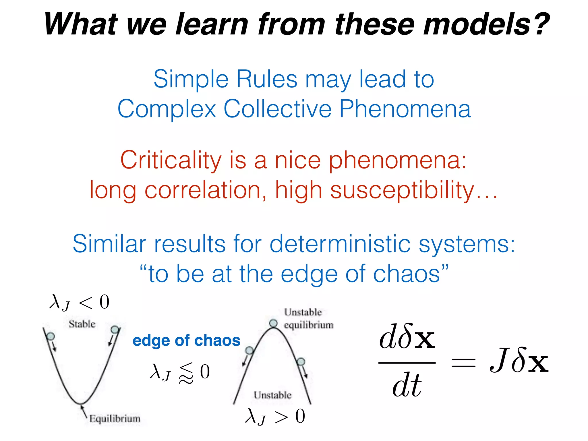
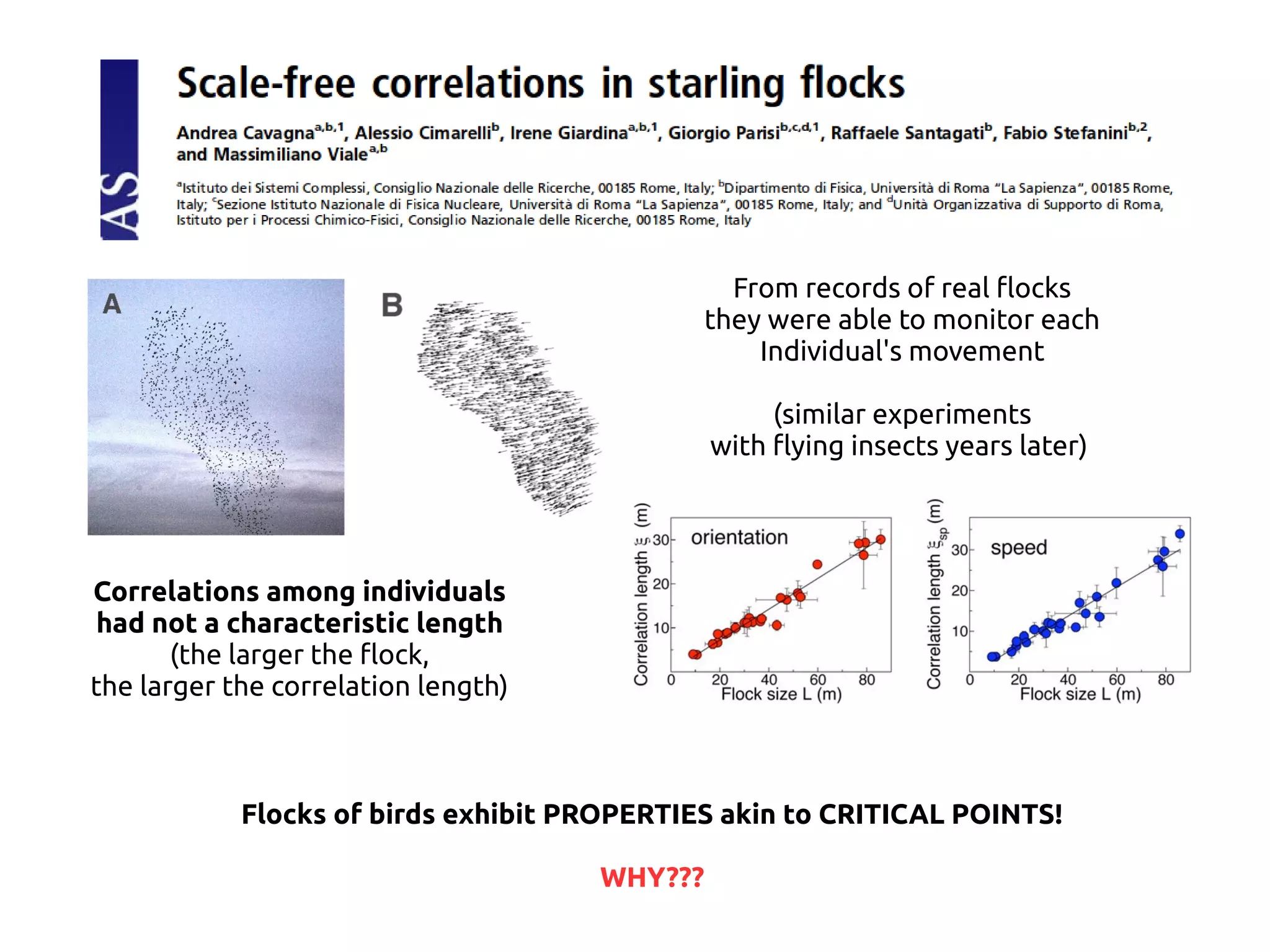
- Systems biology is an interdisciplinary field that studies biological systems using a holistic approach, focusing on complex interactions within systems. - Statistical physics approaches, like the Ising model of magnetism, can be applied to study biological systems and emergent phenomena. These simple models reveal how complex collective behavior can arise from local interactions. - Critical phenomena observed in models like the Ising model provide insights into how biological systems may benefit from operating near a critical point, with long-range correlations and sensitivity to perturbations.