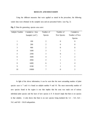
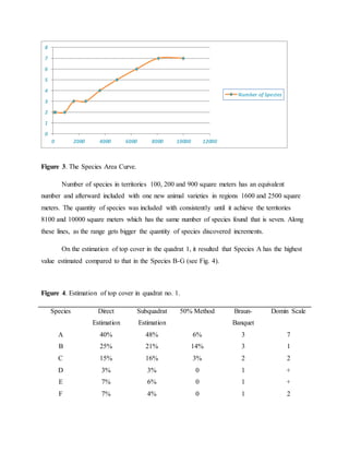
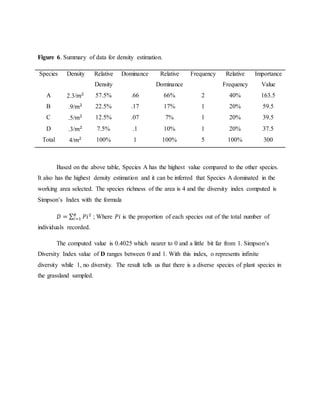
This document summarizes a scientific study that analyzed plant species abundance and diversity in a grassland ecosystem in Iligan City, Philippines. Quadrats and transect lines were used to sample vegetation and record data on species area curves, cover estimates, density, and diversity. Results showed species richness increased with area. One species, Species A, dominated the area based on cover and density estimates. The species richness was 4 and Simpson's Diversity Index value was 0.4025, indicating diverse plant species in the grassland.

1. AN ANALYZATION OF THE ABUNDANCE AND DIVERSITY
OF PLANT SPECIES IN GLOBAL STEEL SOCCER FIELD
GRASSLAND ECOSYSTEM, ILIGAN CITY
-------------------------
A Scientific Paper
Presented to:
Prof. Karyl Fabricante-Dagoc
Department of Biological Sciences
CSM, MSU – IIT
--------------------------
Presented by:
Mary Glydel P. Florin
In Partial Fulfilment of the course Bio 107.2
General Ecology Laboratory
Second Semester A.Y 2015-2016

2. ACKNOWLEDGEMENTS
I would like to express my profound gratitude to a number of people who cooperated in
performing the experiment. Aside from my effort as the researcher in completing this paper, the
accomplishment of this field sampling depended largely on the encouragement and guidelines of
many others. To my instructor, Prof. Karyl Fabricante-Dagoc, thank you for your extended
patience, and above all, to God be all the glory.

3. ABSTRACT
Grasslands are terrains with regular grass spreads, bushes and not very abundant secluded
trees. These grounds are predominantly utilized for cows eating and raising animals. The
fundamental motivation behind this study is to dissect the vegetation found on the chosen area.
Our point is to decide the species area curve, spread estimation of vegetation and density
estimation in the grassland community. Using quadrats for plot testing and the transect line for
transect inspecting strategies, information and results were recorded. A 10-m transect line was
laid and the 1 square meter quadrat was put toward the end of the 10m transect line and number
of species were tallied. Results demonstrate that the species area curve is directly proportional to
the quantity of species present, thus, the number species increases as the area sampled expands.
For the estimation of top spread, it is found that one species of plant is abundant than other types
of plant in the field. The thickness estimation yields similar results. The Species Richness during
the conduction of zonation and thickness estimation was 4 and the figured assorted qualities
record (Simpson's Index) worth is 0.4025 which suggests that the species in the Global Steel
Soccer Field Grassland ecosystem is diverse.

4. INTRODUCTION
Grassland ecosystem is a field where grasses are the dominant flora and is composed of
other plants, animals and micro-organisms that utilized the zone as their habitat. It occurs in
places which are excessively dry for a forest, but have sufficient soil water to support a closed
herbaceous plant covering that is lacking in desserts. In tropical and subtropical grasslands the
length of the growing season is determined by how long the rainy season lasts. But in the
temperate grasslands the length of the growing season is determined by temperature. Plants
usually start growing when the daily temperature reached about 50° F. (Sam M., 2000)
The intentions of this study are to train the students on the principles of plot and transect
sampling as correlated in ecological research and determine the diversity of plant species in a
grassland ecosystem, species area curve, cover and density estimates. This also aims to construct
a zonation diagram of a grassland ecosystem and helps the students to be able to illustrate the
connotation of different combined parameters. By using this method, important parameters can
be estimated and quantified which include the areas’ density, frequency and important value of
constitutive species.
In this experiment, the usage of plot sampling to analyse methods of vegetation will be
introduced. This method is utilized for acquiring tests samples of both terrestrial and aquatic
such as plants and slow moving organisms for example. Quadrat size will rely on the type of
vegetation to be sampled. For short grassland, a range from 0.5 to 1.0𝑚2
quadrats is suggested
and 2m quadrats might be the minimum requirement for taller grassland and shrubby habitat.

5. MATERIALS AND METHODS
A. Sampling Area
The fieldwork sampling was administered at Global Steel Soccer Field, Suarez, Iligan
City (Figure 1) on March 12, 2016, starting from 7:00 am to 9:00 am.
Figure 1. Actual photo of the grassland field.
In the preparation for the species area curve, each group in the class randomly selected
an area in the grassland field to be sampled. Plant species present in the subquadrat that is 10 cm
X 10 cm within the 1 square meter quadrat was counted and recorded. The size of the subquadrat
was doubled and the results were again recorded. The doubling and counting was repeated until
the number of species counted at each doubling of subquadrat size no longer gave any species.
In acquiring the cover estimation of vegetation, the area covered with grasses (top
cover) was visually estimated in each of the 1 m2 quadrat and the results were recorded.

6. a. Direct Estimation of Top Cover
The top cover was visually estimated by the students for the whole quadrat. The species
observed were recorded to the nearest percent, thus, the total for all species and bare ground
equalled to 100%.
b. Subquadrat Estimation of Top Cover
The results of the estimated percentage cover of each species found in the 25 of the 100
10 cm x 10 cm subquadrat were added and then the mean to obtain an estimate of the top cover
percentages for 1𝑚2
quadrat was calculated.
c. 50% Method
In the 50% method, 100 subquadrats were obtained, thus, species in the quadrat occupies
greater than or equal to 50%. The summed values for this method often lie below 100% since
many subquadrats contain a species mix where no single species (or bare ground) will reach
50%.
d. Braun – Blanquet 5 Point Scale
The top cover of each plant species was estimated visually and the bare ground for the
five 1 m2 plot using the following scale:
+very rare less than 1%
1 rare 1-5%
2 occasional 6-25%
3 frequent 26-50%

7. 4 Common 51-75%
5 abundant 76-100%
e. Domin Scale
The top cover was visually estimated of each species in 1 m x 1 m meter plot using the
following scale:
+ A single individual
1 Scarce, 1-2 individuals
2 Very scattered, cover small less than 1%
3 Scattered, cover small 1-4%
4 Abundant, cover 5-10%
5 Abundant, cover 11-25%
6 Abundant, cover 26-33%
7 Abundant, cover 34-50%
8 Abundant, cover 51-75%
9 Abundant, cover greatly than 75% but not complete
10 Cover practically complete
In deciding the Zonation and Density estimation, the calibrated 10 m transect line was
set down over the study zone by connecting two randomly selected points. Transect line must be
no less than 5m separation from those of different gatherings. The quantity of plants captured by
the transect line were checked and distinguished. Start toward one side of the line. It

8. incorporated those plants whose arial foliage overlies the transect line and those that are touched
by the line or blocked inside of a 1 cm portion of the line. The separation captured by every plant
in the line was measured with the utilization of the Tape measure. In making the Zonation
outline, sections were utilized to demonstrate the captured separation. Plant stature, kind of
substrate and profundity of standing water if present, might likewise be noted. Likewise, the side
and top perspective pictures must be illustrated.
In the density estimation, a 100 m transect line was established across the study area, that
is extending perpendicularly starting at one meter from the trail. A 1 m2 quadrat was plotted at
the end of each 10 m transect line with each of the species being counted. The quadrat was
repositioned at the end of the next transect line. Number of species was again estimated at each
new position in order for the total to be 10 sampling units or quadrats for the entire study area.
All observed data were recorded accordingly. Computation thus follows. (See figure 1b. in
Appendix A for the formula used in the computation.)

9. RESULTS AND DISCUSSION
Using the different measures that were applied as stated in the procedure, the following
varied data were obtained in the sampled area and are presented below. (see Fig. 2)
Fig. 2 Data for generating species area curve
Subplot Number Cumulative Area
Sampled (𝑐𝑚2
)
Number of
Species
Number of
New Species
Cumulative
Number of New
Species
1 100 2 0 0
2 200 2 0 0
3 900 2 0 0
4 1600 3 1 1
5 2500 3 0 1
6 3600 4 1 2
7 4900 5 1 3
8 6400 6 1 4
9 8100 7 1 5
10 10000 7 0 5
In light of the above information, it can be seen that the most astounding number of plant
species seen is 7 and it is found on subplot number 9 and 10. The most noteworthy number of
new species found in the region is one that implies that the zone was made out of various
individual plant species and the least of new species is 0. It doesn't imply that there is no species
in that subplot, it only shows that there is no new species being included the 1x1 - 3x3, 4x4 -
5x5, and 9x9 - 10x10 subquadrats.

10. Figure 3. The Species Area Curve.
Number of species in territories 100, 200 and 900 square meters has an equivalent
number and afterward included with one new animal varieties in regions 1600 and 2500 square
meters. The quantity of species was included with consistently until it achieve the territories
8100 and 10000 square meters which has the same number of species found that is seven. Along
these lines, as the range gets bigger the quantity of species discovered increments.
On the estimation of top cover in the quadrat 1, it resulted that Species A has the highest
value estimated compared to that in the Species B-G (see Fig. 4).
Figure 4. Estimation of top cover in quadrat no. 1.
Species Direct
Estimation
Subquadrat
Estimation
50% Method Braun-
Banquet
Domin Scale
A 40% 48% 6% 3 7
B 25% 21% 14% 3 1
C 15% 16% 3% 2 2
D 3% 3% 0 1 +
E 7% 6% 0 1 +
F 7% 4% 0 1 2
0
1
2
3
4
5
6
7
8
0 2000 4000 6000 8000 10000 12000
Number of Species

11. G 3% 2% 0 1 1
In the above table, it can be inferred that Species A had dominated the area being
conducted in the sample compared to the other species B-G. Species A was abundant in the area
that the rest of the species from B-G.
The zonation diagrams below are constructed using the data collected for the zonation
and density estimation (see Appendix A).
Figure 5. Zonation diagram of plant species showing intercepted length covered by each plant.
Side view
Top view
Species 1 Species 2 Species 3 Species 4 Species 1
Species 1 Species 2 Species 3 Species 4 Species 1

12. Figure 6. Summary of data for density estimation.
Species Density Relative
Density
Dominance Relative
Dominance
Frequency Relative
Frequency
Importance
Value
A 2.3/𝑚2 57.5% .66 66% 2 40% 163.5
B .9/𝑚2 22.5% .17 17% 1 20% 59.5
C .5/𝑚2 12.5% .07 7% 1 20% 39.5
D .3/𝑚2 7.5% .1 10% 1 20% 37.5
Total 4/𝑚2 100% 1 100% 5 100% 300
Based on the above table, Species A has the highest value compared to the other species.
It also has the highest density estimation and it can be inferred that Species A dominated in the
working area selected. The species richness of the area is 4 and the diversity index computed is
Simpson’s Index with the formula
𝐷 = ∑ 𝑃𝑖2𝑅
𝑖=1 ; Where 𝑃𝑖 is the proportion of each species out of the total number of
individuals recorded.
The computed value is 0.4025 which nearer to 0 and a little bit far from 1. Simpson’s
Diversity Index value of D ranges between 0 and 1. With this index, o represents infinite
diversity while 1, no diversity. The result tells us that there is a diverse species of plant species in
the grassland sampled.

13. CONCLUSION
The grassland ecosystem prepared the way of the students to encounter the principles of
plot and transect sampling and how it is used as applied in ecological research. These sampling
techniques enable them to get data to determine the species area curve, cover and density
estimates, and the diversity of plant species in a grassland ecosystem.
In the conducted study, taking into account the outcomes, the quantity of species present
in the sampled field ranges from 2-7. It can be gathered that the bigger the region, the bigger
number of species around the area, thus results show that species richness is directly proportional
to the area. In the estimation of top cover and the tabulation of raw data for density estimation, it
can be inferred that Species A had dominated the area being conducted compared to that of the
other species found within the transect line. Thus, species A was abundant in the area being
conducted and selected and had dominated it. Species A also had the greatest Importance Value
which could mean of it being the keystone species in the grassland ecosystem.

14. RECOMMENDATION
It is highly recommended to study the diversity and abundance of the grassland area
further to obtain better results especially in the Philippines to provide more information of the
different plant species in the grasslands and their abundance for future studies.
Few insufficiencies and some mistakes may include the uncertainty whether the plant
species present inside the quadrat were to be counted or left uncounted because half of its
entirety belongs inside the quadrat while the other belongs to the outside quadrat.

15. APPENDIX A
Figure 1b
C. Zonation and Density Estimation
Density of a species = No. of individuals of a species
Total area sampled
Relative Density = Density of a species . x 100
Total density of all species
Dominance of a species = Total area covered by a species
Total area sampled
Relative Dominance = Dominance of a species x 100 s
Total dominance of all species
Frequency of a species= number of quadrats where a species occurs
Relative Frequency = Frequency value for a species . x 100
Total frequency of all species
Importance Value= Relative Density= Relative Dominance+ Relative Frequency
The data from the different sampling techniques on the species composition and number
of individuals per species was computed using the Simpson’s and Shannon- Weiner’s Indices
for measuring diversity.
D. Diversity Measurements
Simpson’s Index 𝐷 = ∑ 𝑃𝑖2𝑅
𝑖=1
Shannon- Weiner Index HꞋ = - ∑ 𝑝₁𝑅
𝑖=1 𝑙𝑜𝑔 p₁

16. Where, Pi is the proportion of each species out of the total number of individuals
recorded. It can also be computed and analysed using the PAST software for an easier way
Figure 2. Raw data for Species Area Curve
Subquadrat Number of
Species
1x1 2
2x2 2
3x3 2
4x4 3
5x5 3
6x6 4
7x7 5
8x8 6
9x9 7
10x10 7
Figure 3. Raw data for Subquadrat Estimation of top cover
Species 1st subquadrat
(%)
2nd subquadrat
(%)
3rd subquadrat
(%)
4th subquadrat
(%)
A 44 43 43 63
B 24 15 26 17
C 16 32 16 0
D 6 2 2 2
E 6 5 5 9
F 4 3 4 5
G 0 0 4 4
Figure 4. Raw data for zonation and Density Estimation
Species Number of Individuals Height (cm)
A 23 25
B 9 85
C 5 7
D 3 77

17. REFERENCES
"Temperate Grasslands" Retrieved on April 3, 2016 from:
http://www.runet.edu/~swoodwar/CLASSES/GEOG235/biomes/tempgrass/tempgras.
html, (Oct. 2000).
"Grasslands", Retrieved on April 3, 2016 from:
http://www.ucmp.berkeley.edu/glossary/gloss5/biome/grasslan.html, (Oct. 2000).
“Grassland Ecosystem” Retrieved on April 3, 2016 from:
http://www.blueplanetbiomes.org/grasslands.htm