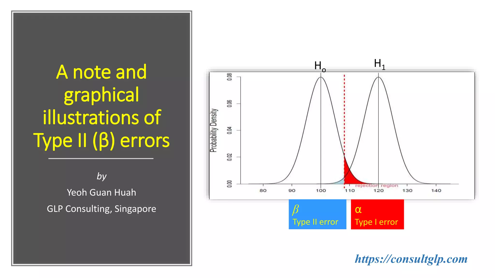
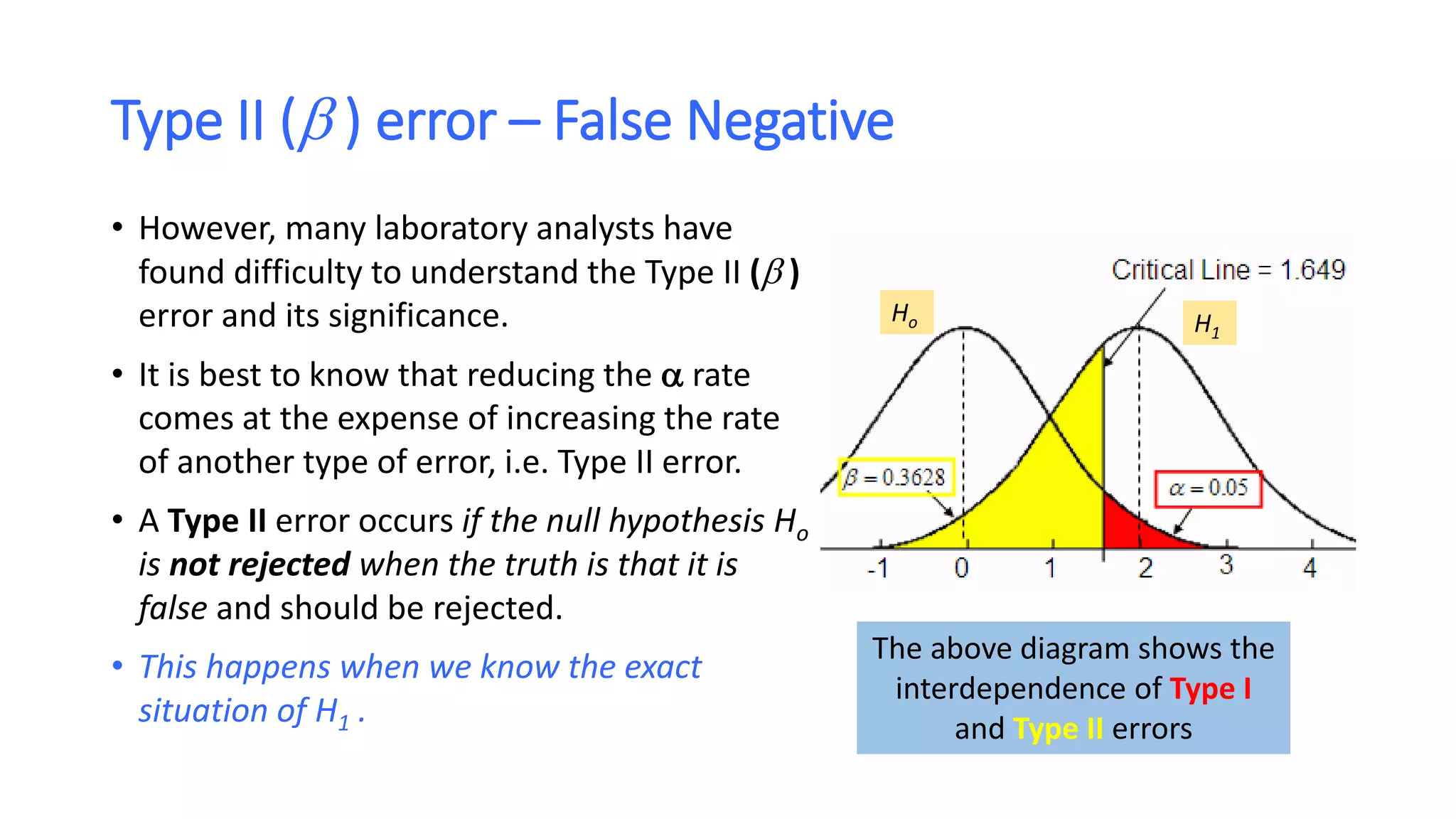
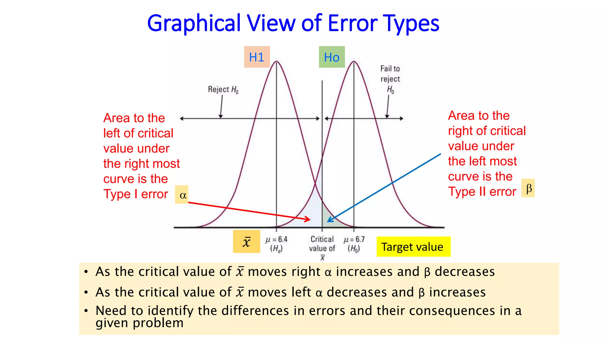
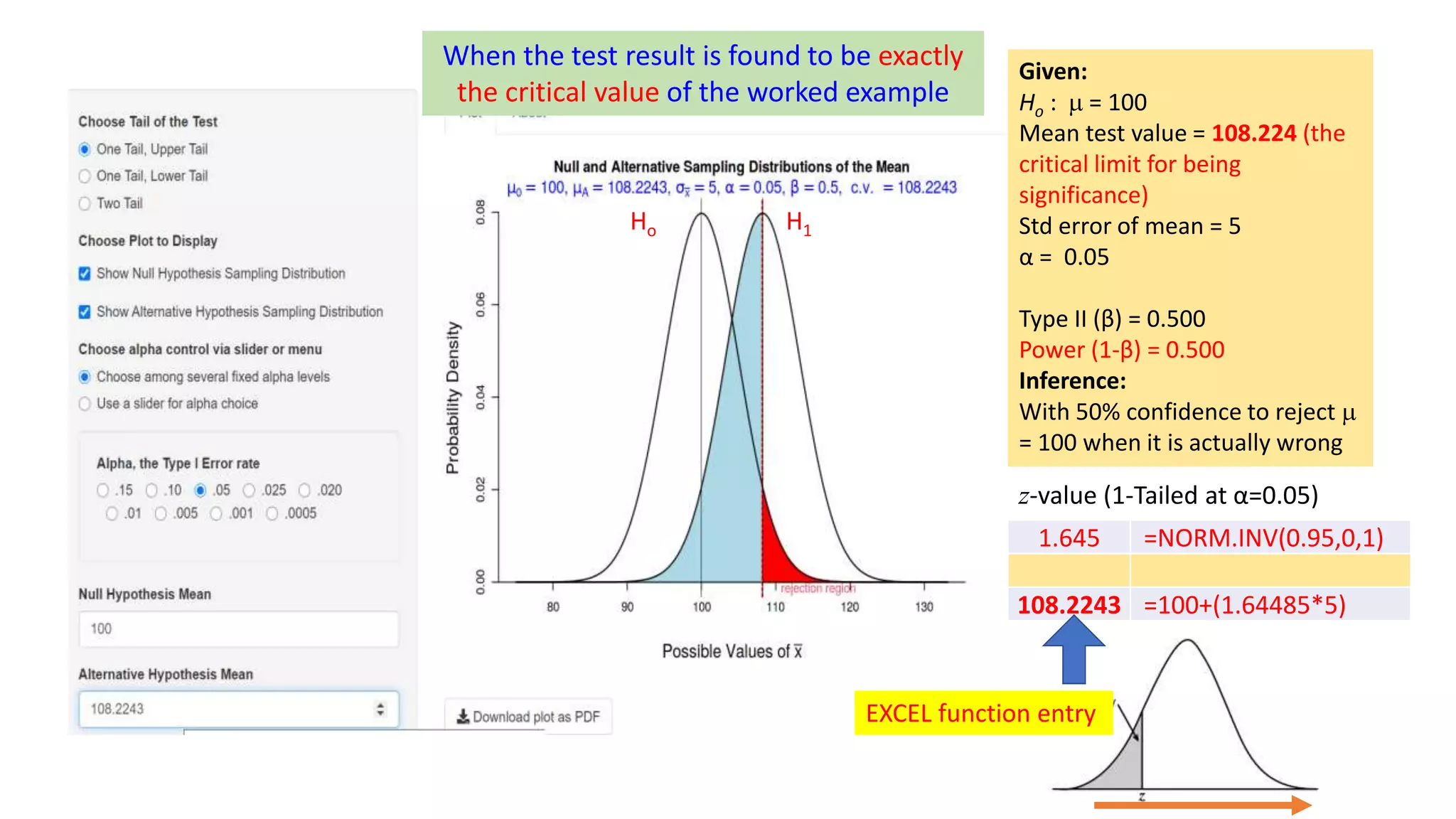
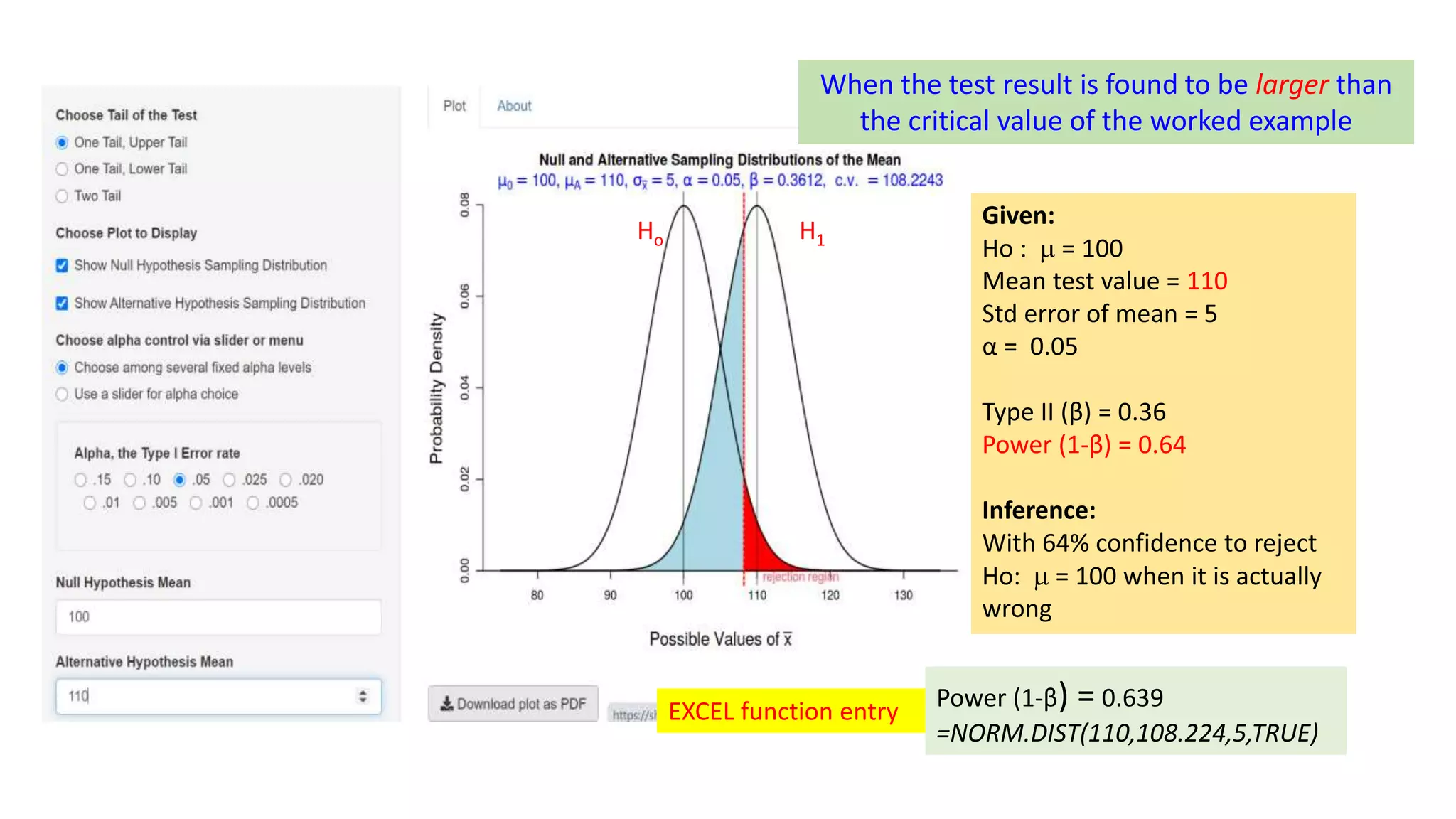
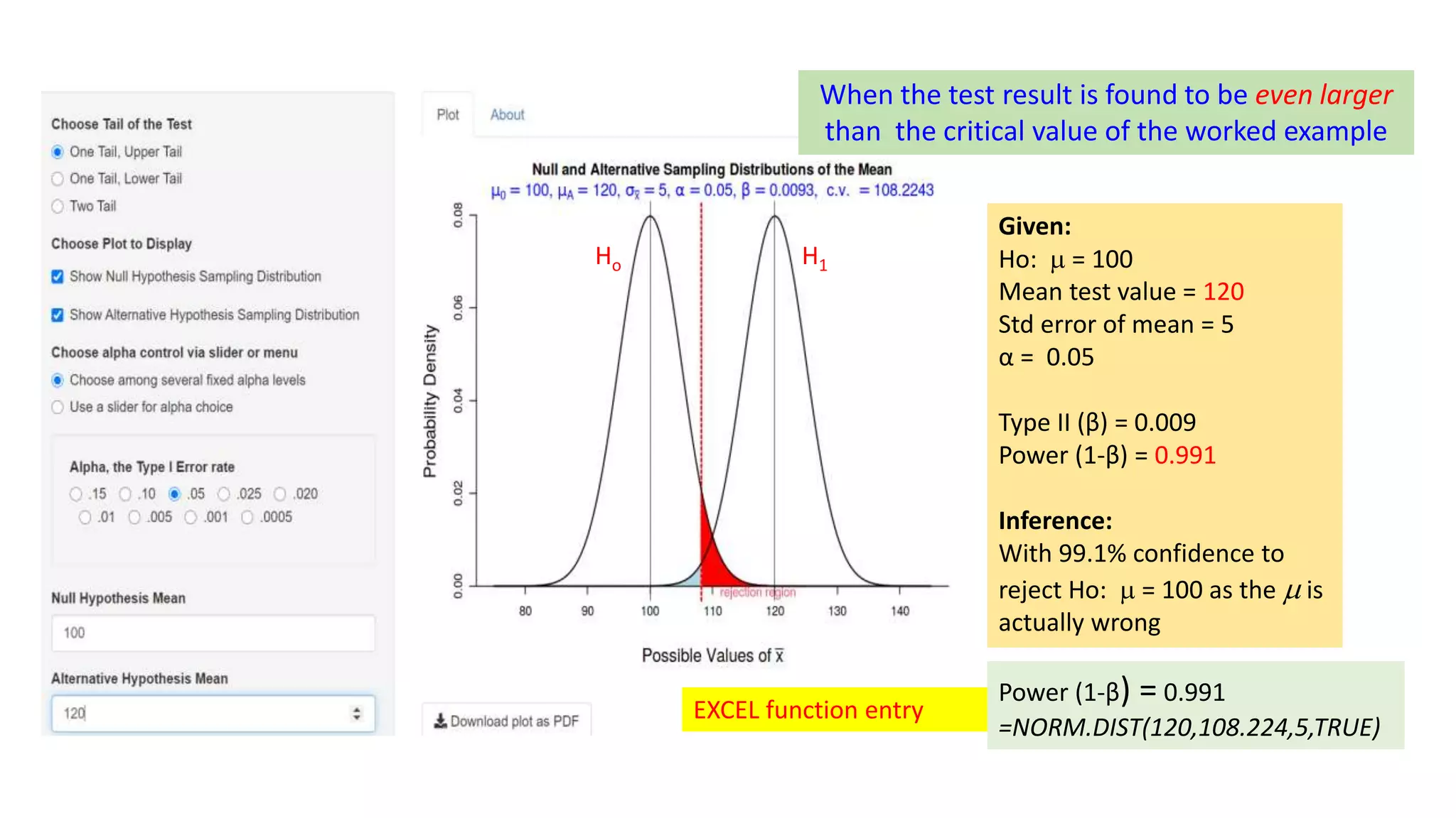
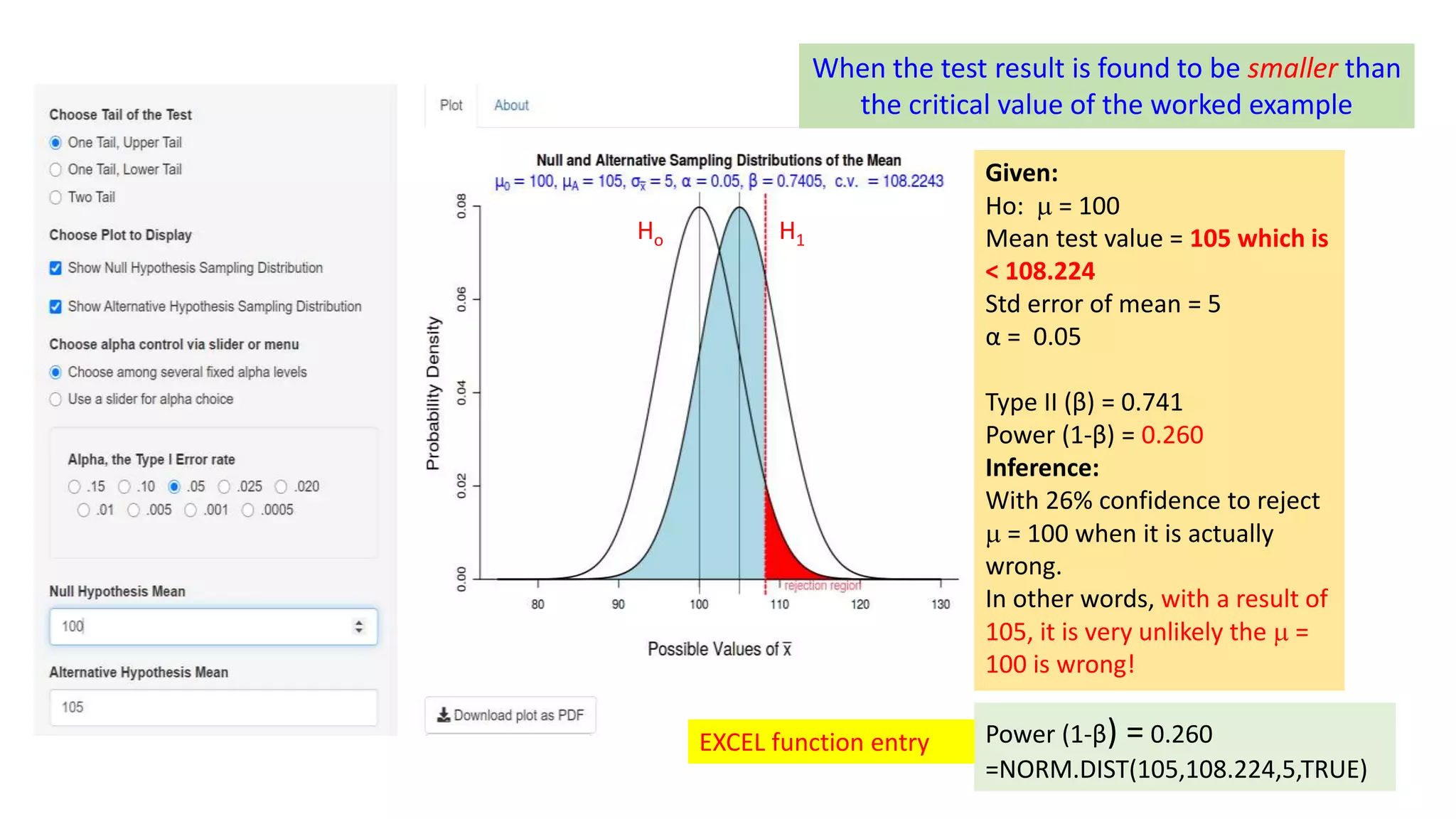
A note and
graphical
illustrations of
Type II (β) errors
by
Yeoh Guan Huah
GLP Consulting, Singapore α
Type I error
β
Type II error
Ho
H1
https://consultglp.com
Introduction
• When we are using a sample statistic to make decisions about a
population parameter, we run into a risk that an incorrect conclusion
might be reached.
• In product conformance testing, when we make a decision rule on
whether a measurement is in compliance with a specification limit, a
certain threshold or a regulatory control limit, we have a risk of
making an incorrect conclusion: either falsely accept or falsely reject
the situation.
• To make a decision, we can do a hypothesis testing. There are 2
different types of errors which can occur for carrying out this test.
• These are referred to as type I and type II errors.
Types of errors and level of significance
• No matter which hypothesis represents the claim, we always
begin a hypothesis test by assuming that the equality condition
in the null hypothesis Ho is true.
• So, in performing a hypothesis test, we make one of the two decisions:
• Reject the null hypothesis, or
• Fail to reject the null hypothesis (i.e. accepting the alternative
hypothesis H1 or Ha.
• As the decision is based on a sample rather than the entire
population, there is always a possibility that we will make a wrong
decision:
• We might reject a null hypothesis when it is actually true.
• Or, we might fail to reject a null hypothesis when it is actually false.
Type I and Type II errors
• A type I ( ) error consists of rejecting the null hypothesis H0 when it
is true. Normally we ‘control’ the probability of making a type I error
by fixing  = 0.05, 0.01, etc., depending on our confidence level.
• A type II ( ) error consists of not rejecting H0 when H0 is false.
• Note: Statisticians often recommend to use statement “do not reject
H0” instead of “accept H0”, because of uncertainty associated with
making a type II error. Using this no rejection statement, we may
have to withhold judgment and action.
•  and  are the probabilities of type I and type II error, respectively.
Type I (α) error – False Positive
• Most laboratory analysts do understand the meaning of Type I (α error) and its
significance.
• A Type I error occurs if the null hypothesis Ho is rejected when in fact, it is true
and should not be rejected. The probability that a Type I error occurs is a
prefixed  (level of significance).
• Since the level of significance is specified before the hypothesis test is
performed, the risk of committing a Type I error,  is directly under our control
• Traditionally,  = 0.05 or smaller is selected. So we can have 95% confidence for
not rejecting Ho, i.e. confidence coefficient is 1-0.05 = 0.95.
• Once an  level is selected, the critical value or values that divide the rejection
from the non-rejection region(s) are then determined (either by z- or t-values
for normal distribution or t-distribution, respectively).
Type II ( ) error – False Negative
• However, many laboratory analysts have
found difficulty to understand the Type II ( )
error and its significance.
• It is best to know that reducing the  rate
comes at the expense of increasing the rate
of another type of error, i.e. Type II error.
• A Type II error occurs if the null hypothesis Ho
is not rejected when the truth is that it is
false and should be rejected.
• This happens when we know the exact
situation of H1 .
The above diagram shows the
interdependence of Type I
and Type II errors
Ho H1
 error and power of statistics (1 -  )
• If the difference between the hypothesized value and the actual corresponding
population parameter measured is large, , the probability of committing a
Type II error, will likely be small.
• From confidence point of view, we report its statistical power, which is a
complement of , i.e. ( 1-  )
• Statistical Power
• Statistical power: the probability of not making a type II ( ) error. It represents
the probability that we reject the null hypothesis when it is false. Power = 1 - 
• In other words, power is the probability that the data gathered in an
experiment will be sufficient to reject a wrong null hypothesis Ho.
Graphical View of Error Types
• As the critical value of 𝑥 moves right α increases and β decreases
• As the critical value of 𝑥 moves left α decreases and β increases
• Need to identify the differences in errors and their consequences in a
given problem
Area to the
left of critical
value under
the right most
curve is the
Type I error
Area to the
right of critical
value under
the left most
curve is the
Type II error
HoH1

Target value𝑥
Some worked examples to
show different situations of
Type II ( ) error
Given:
Ho :  = 100
Mean test value = 108.224 (the
critical limit for being
significance)
Std error of mean = 5
α = 0.05
Type II (β) = 0.500
Power (1-β) = 0.500
Inference:
With 50% confidence to reject 
= 100 when it is actually wrong
Ho H1
1.645 =NORM.INV(0.95,0,1)
108.2243 =100+(1.64485*5)
z-value (1-Tailed at α=0.05)
EXCEL function entry
When the test result is found to be exactly
the critical value of the worked example
Given:
Ho :  = 100
Mean test value = 110
Std error of mean = 5
α = 0.05
Type II (β) = 0.36
Power (1-β) = 0.64
Inference:
With 64% confidence to reject
Ho:  = 100 when it is actually
wrong
Ho H1
When the test result is found to be larger than
the critical value of the worked example
Power (1-β) = 0.639
=NORM.DIST(110,108.224,5,TRUE)
EXCEL function entry
Given:
Ho:  = 100
Mean test value = 120
Std error of mean = 5
α = 0.05
Type II (β) = 0.009
Power (1-β) = 0.991
Inference:
With 99.1% confidence to
reject Ho:  = 100 as the  is
actually wrong
Ho H1
When the test result is found to be even larger
than the critical value of the worked example
Power (1-β) = 0.991
=NORM.DIST(120,108.224,5,TRUE)
EXCEL function entry
Given:
Ho:  = 100
Mean test value = 105 which is
< 108.224
Std error of mean = 5
α = 0.05
Type II (β) = 0.741
Power (1-β) = 0.260
Inference:
With 26% confidence to reject
 = 100 when it is actually
wrong.
In other words, with a result of
105, it is very unlikely the  =
100 is wrong!
Ho H1
When the test result is found to be smaller than
the critical value of the worked example
Power (1-β) = 0.260
=NORM.DIST(105,108.224,5,TRUE)
EXCEL function entry
Conclusion
• Whilst we can control our risk to wrongly reject a null hypothesis Ho
when it is true by fixing the Type I (α) error magnitude, any attempt
to reduce this  rate comes at the expense of increasing the rate of
another type of error, namely Type II (β ) error. This is because type I
is not the only possible type of error in hypothesis testing.
• In fact, Type II error is not difficult to understand if we remember the
very point that it is an error measured when we had accepted a false
null hypothesis.
• The magnitude of Type II error can be confirmed if the actual test
value is found to be significantly larger or smaller than the critical
value on the right hand tail or left hand tail of the normal distribution
curve, respectively.

A note and graphical illustration of type II error

  • 1.
    A note and graphical illustrationsof Type II (β) errors by Yeoh Guan Huah GLP Consulting, Singapore α Type I error β Type II error Ho H1 https://consultglp.com
  • 2.
    Introduction • When weare using a sample statistic to make decisions about a population parameter, we run into a risk that an incorrect conclusion might be reached. • In product conformance testing, when we make a decision rule on whether a measurement is in compliance with a specification limit, a certain threshold or a regulatory control limit, we have a risk of making an incorrect conclusion: either falsely accept or falsely reject the situation. • To make a decision, we can do a hypothesis testing. There are 2 different types of errors which can occur for carrying out this test. • These are referred to as type I and type II errors.
  • 3.
    Types of errorsand level of significance • No matter which hypothesis represents the claim, we always begin a hypothesis test by assuming that the equality condition in the null hypothesis Ho is true. • So, in performing a hypothesis test, we make one of the two decisions: • Reject the null hypothesis, or • Fail to reject the null hypothesis (i.e. accepting the alternative hypothesis H1 or Ha. • As the decision is based on a sample rather than the entire population, there is always a possibility that we will make a wrong decision: • We might reject a null hypothesis when it is actually true. • Or, we might fail to reject a null hypothesis when it is actually false.
  • 4.
    Type I andType II errors • A type I ( ) error consists of rejecting the null hypothesis H0 when it is true. Normally we ‘control’ the probability of making a type I error by fixing  = 0.05, 0.01, etc., depending on our confidence level. • A type II ( ) error consists of not rejecting H0 when H0 is false. • Note: Statisticians often recommend to use statement “do not reject H0” instead of “accept H0”, because of uncertainty associated with making a type II error. Using this no rejection statement, we may have to withhold judgment and action. •  and  are the probabilities of type I and type II error, respectively.
  • 5.
    Type I (α)error – False Positive • Most laboratory analysts do understand the meaning of Type I (α error) and its significance. • A Type I error occurs if the null hypothesis Ho is rejected when in fact, it is true and should not be rejected. The probability that a Type I error occurs is a prefixed  (level of significance). • Since the level of significance is specified before the hypothesis test is performed, the risk of committing a Type I error,  is directly under our control • Traditionally,  = 0.05 or smaller is selected. So we can have 95% confidence for not rejecting Ho, i.e. confidence coefficient is 1-0.05 = 0.95. • Once an  level is selected, the critical value or values that divide the rejection from the non-rejection region(s) are then determined (either by z- or t-values for normal distribution or t-distribution, respectively).
  • 6.
    Type II () error – False Negative • However, many laboratory analysts have found difficulty to understand the Type II ( ) error and its significance. • It is best to know that reducing the  rate comes at the expense of increasing the rate of another type of error, i.e. Type II error. • A Type II error occurs if the null hypothesis Ho is not rejected when the truth is that it is false and should be rejected. • This happens when we know the exact situation of H1 . The above diagram shows the interdependence of Type I and Type II errors Ho H1
  • 7.
     error andpower of statistics (1 -  ) • If the difference between the hypothesized value and the actual corresponding population parameter measured is large, , the probability of committing a Type II error, will likely be small. • From confidence point of view, we report its statistical power, which is a complement of , i.e. ( 1-  ) • Statistical Power • Statistical power: the probability of not making a type II ( ) error. It represents the probability that we reject the null hypothesis when it is false. Power = 1 -  • In other words, power is the probability that the data gathered in an experiment will be sufficient to reject a wrong null hypothesis Ho.
  • 8.
    Graphical View ofError Types • As the critical value of 𝑥 moves right α increases and β decreases • As the critical value of 𝑥 moves left α decreases and β increases • Need to identify the differences in errors and their consequences in a given problem Area to the left of critical value under the right most curve is the Type I error Area to the right of critical value under the left most curve is the Type II error HoH1  Target value𝑥
  • 9.
    Some worked examplesto show different situations of Type II ( ) error
  • 10.
    Given: Ho : = 100 Mean test value = 108.224 (the critical limit for being significance) Std error of mean = 5 α = 0.05 Type II (β) = 0.500 Power (1-β) = 0.500 Inference: With 50% confidence to reject  = 100 when it is actually wrong Ho H1 1.645 =NORM.INV(0.95,0,1) 108.2243 =100+(1.64485*5) z-value (1-Tailed at α=0.05) EXCEL function entry When the test result is found to be exactly the critical value of the worked example
  • 11.
    Given: Ho : = 100 Mean test value = 110 Std error of mean = 5 α = 0.05 Type II (β) = 0.36 Power (1-β) = 0.64 Inference: With 64% confidence to reject Ho:  = 100 when it is actually wrong Ho H1 When the test result is found to be larger than the critical value of the worked example Power (1-β) = 0.639 =NORM.DIST(110,108.224,5,TRUE) EXCEL function entry
  • 12.
    Given: Ho:  =100 Mean test value = 120 Std error of mean = 5 α = 0.05 Type II (β) = 0.009 Power (1-β) = 0.991 Inference: With 99.1% confidence to reject Ho:  = 100 as the  is actually wrong Ho H1 When the test result is found to be even larger than the critical value of the worked example Power (1-β) = 0.991 =NORM.DIST(120,108.224,5,TRUE) EXCEL function entry
  • 13.
    Given: Ho:  =100 Mean test value = 105 which is < 108.224 Std error of mean = 5 α = 0.05 Type II (β) = 0.741 Power (1-β) = 0.260 Inference: With 26% confidence to reject  = 100 when it is actually wrong. In other words, with a result of 105, it is very unlikely the  = 100 is wrong! Ho H1 When the test result is found to be smaller than the critical value of the worked example Power (1-β) = 0.260 =NORM.DIST(105,108.224,5,TRUE) EXCEL function entry
  • 14.
    Conclusion • Whilst wecan control our risk to wrongly reject a null hypothesis Ho when it is true by fixing the Type I (α) error magnitude, any attempt to reduce this  rate comes at the expense of increasing the rate of another type of error, namely Type II (β ) error. This is because type I is not the only possible type of error in hypothesis testing. • In fact, Type II error is not difficult to understand if we remember the very point that it is an error measured when we had accepted a false null hypothesis. • The magnitude of Type II error can be confirmed if the actual test value is found to be significantly larger or smaller than the critical value on the right hand tail or left hand tail of the normal distribution curve, respectively.