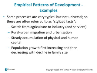
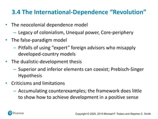
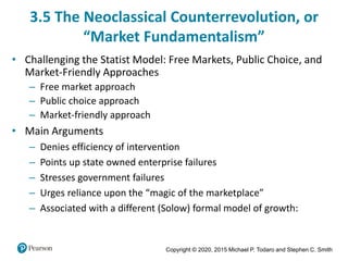
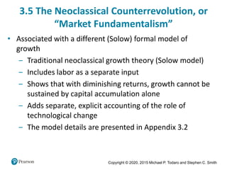
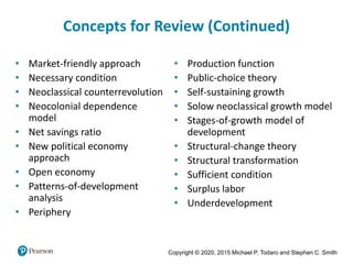
1. The document summarizes several classic theories of economic growth and development, including linear stages of growth, structural change models, dependency theory, and neoclassical counterrevolution theories.
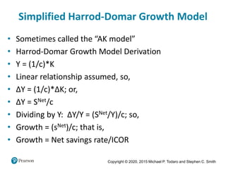
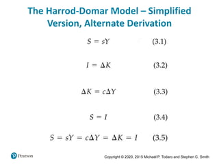
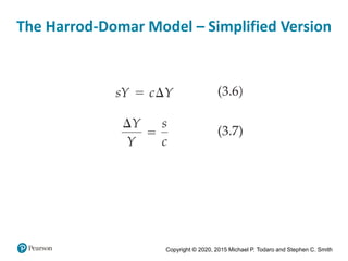
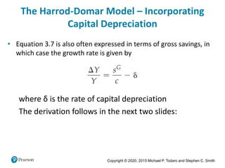
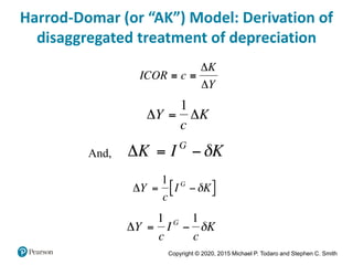
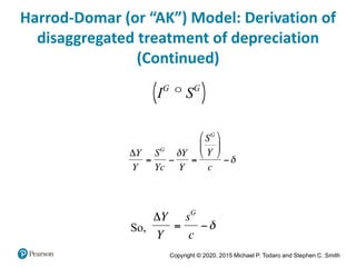
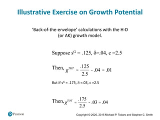
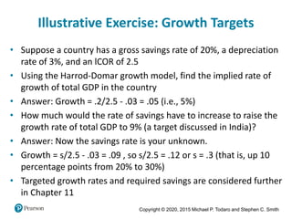
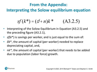
2. It outlines Rostow's stages of growth model and the Harrod-Domar growth model, describing their key assumptions and equations.
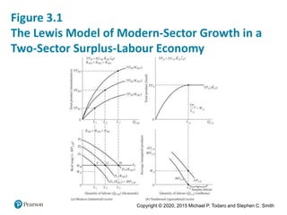
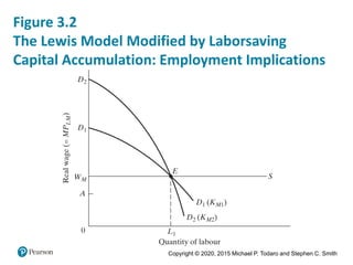
3. Lewis' two-sector model of labor transferring from subsistence agriculture to higher productivity industry is also introduced, along with its limitations.