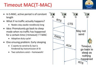
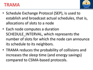
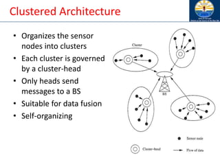
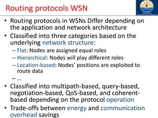
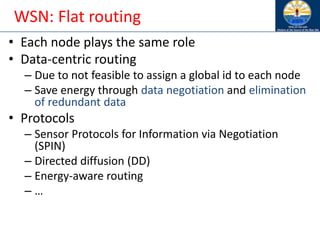
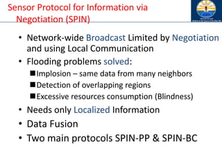
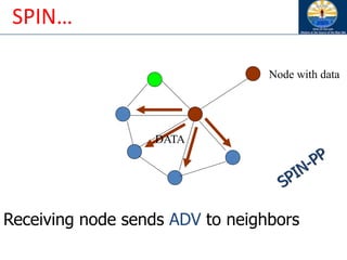
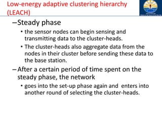
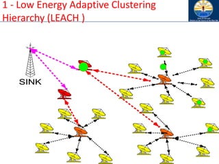
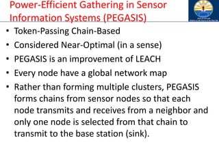
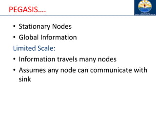
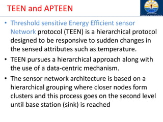
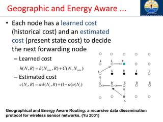
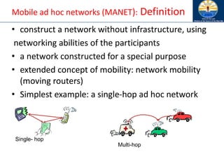
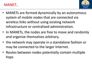
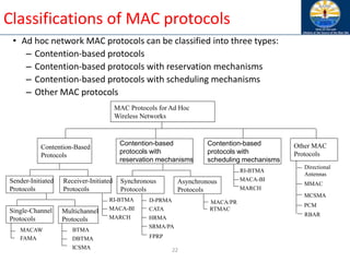
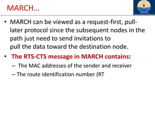
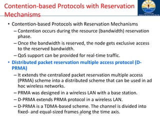
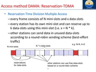
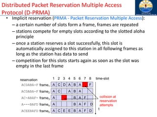
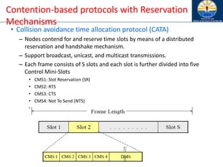
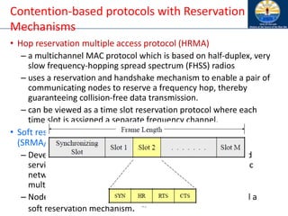
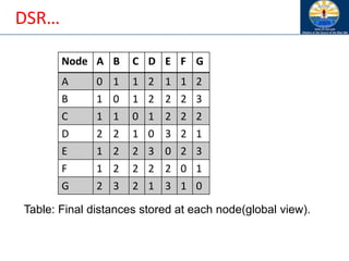
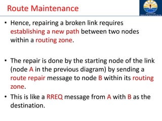
The document discusses mobile ad hoc networks (MANETs) and wireless sensor networks, focusing on their characteristics, functionalities, and protocols. MANETs are decentralized networks that enable communication among mobile nodes without a fixed infrastructure, facing challenges like mobility, energy constraints, and security. It also covers Media Access Control (MAC) protocols designed for efficiency and quality of service in these dynamic environments.

1. 8. Mobile ad hoc and wireless
sensor networks
1 Ad hoc Networks
2 Routing protocols
3 MAC protocol for MANET
4 TCP in ad hoc network
5 Wireless Sensor Networks
S,K.Sarkar, etal., Ad hoc Mobile wireless networks: Pinciples,
protocols and Applications. 2008

2. 1. Ad hoc networks

3. Mobile ad hoc networks (MANET): Definition
• construct a network without infrastructure, using
networking abilities of the participants
• a network constructed for a special purpose
• extended concept of mobility: network mobility
(moving routers)
• Simplest example: a single-hop ad hoc network
Single- hop
Multi-hop

4. MANET..
• MANETs are formed dynamically by an autonomous
system of mobile nodes that are connected via
wireless links without using existing network
infrastructure or centralized administration.
• In MANETs, the nodes are free to move and randomly
and organize themselves arbitrary.
• the network may operate in a standalone fashion or
may be connected to the larger Internet.
• Routes between nodes potentially contain multiple
hops

5. Difference between Cellular and Ad hoc
Wireless Networks
Cellular Ad Hoc Wireless Networks
Infrastructure Networks Infrastructureless Networks
Fixed, prelocated cell sites, and
base station
No base station and rapid
deployment
Static backbone network
topology
Highly dynamic network
topologies with multihop
Relatively caring environment
and stable connectivity
Hostile environment (nosie,
losses) and irregular connectivity
Detailed planning before base
station can be installed
Ad hoc network automatically
forms and adapts to changes
High setup costs Cost-effective
Large setup time Less setup time

6. Characteristics of ad hoc network
• Infrastructure-less or with minimum
infrastructure support
• Self-organizing and self-managing
• Most or some of the nodes are mobile
• Multi-hop
• Energy constraint
• ….

7. Infrastructure-less or with minimum
infrastructure support
• A pure ad hoc network does not have, or simply
does not rely on infrastructure support (for routing,
network management, et al.)
• A hybrid ad hoc network consists of both client
nodes and infrastructure nodes, i.e. nodes whose
function is merely transporting traffic for the client
nodes. Hybrid networks are more common
• Dynamic network topology
– Nodes are mobile, and at any one time there are nodes
joining in or leaving
– Frequent, temporary, and unannounced loss of network
connectivity is common

8. Self-organizing and self-managing
• Without a central entity (like a base station),
participants must organize themselves into a
network (Self organization)
• For example
– Node is both a host and a router
– Medium access control: no base station can assign
transmission resources, must be decided in a
distributed fashion
– Finding a route from one participant to another

9. Most or some of the nodes are mobile
• Mobility calls for suitable, adaptive
protocols
• In many (not all!) ad hoc network
applications, participants move around
– In cellular network: simply hand over to
another base station
• In mobile ad hoc networks (MANET)
– Mobility changes neighborhood r
relationship
– Must be compensated for
– E.g., routes in the network have to be changed
• Complicated by scale
– Large number of such nodes difficult to support

10. Multi-hop
• Limited range --> multi-hopping
• For many scenarios, communication with peers outside
immediate communication range is required
– Direct communication limited because of distance,
obstacle,...
– Solution: multi-hop network

11. Energy Constraint
• Battery-operated devices -> energy-efficient operations
• Often (not always!), participants in an ad hoc network
draw energy from batteries
• Desirable: long run time for
– Individual devices
– Network as as whole
• Energy-efficient networking protocols
– E.g., use multi-hop routes with low energy consumption
(energy/bit)
– E.g., take available battery capacity of devices into
account
– How to resolve conflicts between different optimizations?

12. Many applications
• Personal area networking cell
– cell phone, laptop, ear phone, wrist watch
• Civilian environments
– meeting rooms
– sports stadiums
– groups of boats, small aircraft (wired REALLY impractical!!)
• Emergency operations
– search-and-rescue
– policing and fire fighting
• Sensor networks
– Groups of sensors embedded in the environment or scattered
over a target area

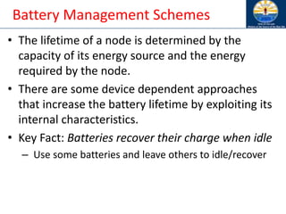
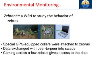
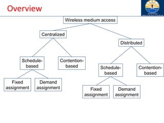
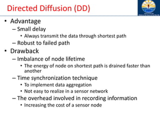
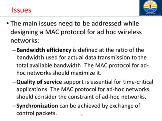
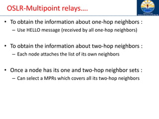
13. Basic Issues
• Mobility: nodes are not fixed at same position
• Energy: nodes may run out of battery and might not be
easy to get to them to recharge
• Scalability [?]: in some applications there is high traffic or
high number of nodes
• Communications limitation of the wireless medium
• Security: depends on the application

14. Problems/challenges for ad hoc
networks
• Without a central infrastructure, things become much
more difficult
• Problems are due to
– Lack of central entity for organization available
– Limited range of wireless communication
– Mobility of participants
– Battery-operated entities
• Ease of snooping on wireless transmissions (security
hazards)
• Sensor networks: resource -constrained

15. Mobility −→ Suitable, adaptive
protocols
• In many (not all!) ad hoc network applications,
participants move around
– In cellular network: simply hand over to another base station
• In mobile ad hoc networks (MANET)
– Mobility changes neighborhood relationship
– Must be compensated for
– E.g., routes in the network have to be changed
• Complicated by scale : Large number of such nodes
difficult to support

16. Battery-operated devices −→ energy-efficient
operation
• Often (not always!), participants in an ad hoc network
draw energy from batteries
• Desirable: long run time for
– Individual devices
– Network as a whole
• −→ Energy-efficient networking protocols
– E.g., use multi-hop routes with low energy consumption
(energy/bit)
– E.g., take available battery capacity of devices into account
– How to resolve conflicts between different optimizations?

17. 2. MAC Protocols for Ad
hoc Wireless Networks

18. 18
Issues
• The main issues need to be addressed while
designing a MAC protocol for ad hoc wireless
networks:
–Bandwidth efficiency is defined at the ratio of the
bandwidth used for actual data transmission to the
total available bandwidth. The MAC protocol for ad-
hoc networks should maximize it.
–Quality of service support is essential for time-critical
applications. The MAC protocol for ad-hoc networks
should consider the constraint of ad-hoc networks.
–Synchronization can be achieved by exchange of
control packets.

19. 19
Issues
• The main issues need to be addressed while designing a
MAC protocol for ad hoc wireless networks:
– Hidden and exposed terminal problems:
• Hidden nodes:
– Hidden stations: Carrier sensing may fail to detect another station.
For example, A and D.
– Fading: The strength of radio signals diminished rapidly with the
distance from the transmitter. For example, A and C.
• Exposed nodes:
– Exposed stations: B is sending to A. C can detect it. C might want to
send to E but conclude it cannot transmit because C hears B.
– Collision masking: The local signal might drown out the remote
transmission.
– Error-Prone Shared Broadcast Channel
– Distributed Nature/Lack of Central Coordination
– Mobility of Nodes: Nodes are mobile most of the time.

20. 20
The 802.11 MAC Sublayer Protocol
(a) The hidden station problem.
(b) The exposed station problem.

21. 21
Design goals of a MAC Protocol
• Design goals of a MAC protocol for ad hoc wireless networks
– The operation of the protocol should be distributed.
– The protocol should provide QoS support for real-time traffic.
– The access delay, which refers to the average delay experienced by any
packet to get transmitted, must be kept low.
– The available bandwidth must be utilized efficiently.
– The protocol should ensure fair allocation of bandwidth to nodes.
– Control overhead must be kept as low as possible.
– The protocol should minimize the effects of hidden and exposed terminal
problems.
– The protocol must be scalable to large networks.
– It should have power control mechanisms.
– The protocol should have mechanisms for adaptive data rate control.
– It should try to use directional antennas.
– The protocol should provide synchronization among nodes.

22. 22
Classifications of MAC protocols
• Ad hoc network MAC protocols can be classified into three types:
– Contention-based protocols
– Contention-based protocols with reservation mechanisms
– Contention-based protocols with scheduling mechanisms
– Other MAC protocols
MAC Protocols for Ad Hoc
Wireless Networks
Contention-Based
Protocols
Contention-based
protocols with
reservation mechanisms
Other MAC
Protocols
Contention-based
protocols with
scheduling mechanisms
Sender-Initiated
Protocols
Receiver-Initiated
Protocols
Synchronous
Protocols
Asynchronous
Protocols
Single-Channel
Protocols
Multichannel
Protocols
MACAW
FAMA
BTMA
DBTMA
ICSMA
RI-BTMA
MACA-BI
MARCH
D-PRMA
CATA
HRMA
RI-BTMA
MACA-BI
MARCH
SRMA/PA
FPRP
MACA/PR
RTMAC
Directional
Antennas
MMAC
MCSMA
PCM
RBAR

23. 23
Classifications of MAC Protocols
• Contention-based protocols
– Sender-initiated protocols: Packet transmissions are initiated by
the sender node.
• Single-channel sender-initiated protocols: A node that wins the contention to the
channel can make use of the entire bandwidth.
• Multichannel sender-initiated protocols: The available bandwidth is divided into
multiple channels.
– Receiver-initiated protocols: The receiver node initiates the
contention resolution protocol.
• Contention-based protocols with reservation
mechanisms
– Synchronous protocols: All nodes need to be synchronized.
Global time synchronization is difficult to achieve.
– Asynchronous protocols: These protocols use relative time
information for effecting reservations.

24. 24
Classifications of MAC Protocols
• Contention-based protocols with scheduling
mechanisms
–Node scheduling is done in a manner so that all nodes
are treated fairly and no node is starved of bandwidth.
–Scheduling-based schemes are also used for enforcing
priorities among flows whose packets are queued at
nodes.
–Some scheduling schemes also consider battery
characteristics.
• Other protocols are those MAC protocols that do
not strictly fall under the above categories.

25. 25
Contention-based protocols
• MACAW: A Media Access Protocol for Wireless LANs is based on
MACA (Multiple Access Collision Avoidance) Protocol
• MACA
– When a node wants to transmit a data packet, it first transmit a RTS
(Request To Send) frame.
– The receiver node, on receiving the RTS packet, if it is ready to receive the
data packet, transmits a CTS (Clear to Send) packet.
– Once the sender receives the CTS packet without any error, it starts
transmitting the data packet.
– If a packet transmitted by a node is lost, the node uses the binary
exponential back-off (BEB) algorithm to back off a random interval of time
before retrying.
• The binary exponential back-off mechanism used in MACA might
starves flows sometimes. The problem is solved by MACAW.

26. 26
MACA Protocol
The MACA protocol. (a) A sending
an RTS to B.
(b) B responding with a CTS to A.

27. 27
• MACA avoids the problem of hidden terminals
– A and C want to
send to B
– A sends RTS first
– C waits after receiving
CTS from B
• MACA avoids the problem of exposed terminals
– B wants to send to A, C
to another terminal
– now C does not have
to wait for it cannot
receive CTS from A
MACA examples
A B C
RTS
CTS
CTS
A B C
RTS
CTS
RTS

28. 28
MACAW
• Variants of this method can be found in IEEE 802.11 as
DFWMAC (Distributed Foundation Wireless MAC),
• MACAW (MACA for Wireless) is a revision of MACA.
– The sender senses the carrier to see and transmits a RTS
(Request To Send) frame if no nearby station transmits a RTS.
– The receiver replies with a CTS (Clear To Send) frame.
– Neighbors
• see CTS, then keep quiet.
• see RTS but not CTS, then keep quiet until the CTS is back to the sender.
– The receiver sends an ACK when receiving an frame.
• Neighbors keep silent until see ACK.
– Collisions
• There is no collision detection.
• The senders know collision when they don’t receive CTS.
• They each wait for the exponential backoff time.

29. 29
MACA variant: DFWMAC in IEEE802.11
idle
wait for the
right to send
wait for ACK
sender receiver
packet ready to send; RTS
time-out;
RTS
CTS; data
ACK
RxBusy
idle
wait for
data
RTS; RxBusy
RTS;
CTS
data;
ACK
time-out 
data;
NAK
ACK: positive acknowledgement
NAK: negative acknowledgement
RxBusy: receiver busy
time-out 
NAK;
RTS

30. 30
Contention-based protocols
• Floor acquisition Multiple Access Protocols (FAMA)
– Based on a channel access discipline which consists of a carrier-
sensing operation and a collision-avoidance dialog between the
sender and the intended receiver of a packet.
– Floor acquisition refers to the process of gaining control of the
channel. At any time only one node is assigned to use the
channel.
– Carrier-sensing by the sender, followed by the RTS-CTS control
packet exchange, enables the protocol to perform as efficiently
as MACA.
– Two variations of FAMA
• RTS-CTS exchange with no carrier-sensing uses the ALOHA protocol for
transmitting RTS packets.
• RTS-CTS exchange with non-persistent carrier-sensing uses non-
persistent CSMA for the same purpose.

31. 31
Contention-based protocols
• Busy Tone Multiple Access Protocols (BTMA)
– The transmission channel is split into two:
• a data channel for data packet transmissions
• a control channel used to transmit the busy tone signal
– When a node is ready for transmission, it senses the channel to
check whether the busy tone is active.
• If not, it turns on the busy tone signal and starts data transmissions
• Otherwise, it reschedules the packet for transmission after some
random rescheduling delay.
• Any other node which senses the carrier on the incoming data channel
also transmits the busy tone signal on the control channel, thus,
prevent two neighboring nodes from transmitting at the same time.
• Dual Busy Tone Multiple Access Protocol (DBTMA) is an
extension of the BTMA scheme.
– a data channel for data packet transmissions
– a control channel used for control packet transmissions (RTS and
CTS packets) and also for transmitting the busy tones.

32. DBTMA..
• Uses two busy tone on the control channel BTt
(Transmitbusy tone) and BTr (Receive busy tone)
are used to notify neighboring nodes of any on-
going transmission.
– BT(t) used by the node that transmits data over the
data channel
– BT(r) used by the node receiving data

33. DBTMA…

34. 34
Contention-based protocols
• Receiver-Initiated Busy Tone Multiple Access Protocol (RI-BTMA)
– The transmission channel is split into two:
• a data channel for data packet transmissions
• a control channel used for transmitting the busy tone signal
– A node can transmit on the data channel only if it finds the busy
tone to be absent on the control channel.
– The data packet is divided into two portions: a preamble and the
actual data packet.
• MACA-By Invitation (MACA-BI) is a receiver-initiated MAC
protocol.
– By eliminating the need for the RTS packet it reduces the number
of control packets used in the MACA protocol which uses the
three-way handshake mechanism.
• Media Access with Reduced Handshake (MARCH) is a receiver-
initiated protocol.

35. MACA -BI
MACA -BI
MACA

36. Media Access with Reduced
Handshake: MARCH
• MARCH exploits the overhearing characteristic
associated with an ad hoc mobile network employing
omni-directional antenna.
• MARCH is a sender and receiver initiated protocol
• MARCH supports fast data transfer over a multi-hop
route
• MARCH provides data flow control by using a
sequence number contained inside the CTS packet
• Improves communication throughput in wireless
multihop Ad-hoc networks by reducing the amount of
control overhead.

37. MARCH;
• In MARCH, a node has knowledge of data packet arrivals at its
neighboring nodes from the overheard CTS packets. It can then
initiate an invitation for data to be relayed.
• Node C will receive the CTS 1 message sent by node B.
• Subsequently, after the data packet has been received by node B,
node C can invite node B to forward that data via the CTS2 packet.
Hence, the RTS 2 packet can be suppressed here.

38. MARCH…
• MARCH can be viewed as a request-first, pull-
later protocol since the subsequent nodes in the
path just need to send invitations to
pull the data toward the destination node.
• The RTS-CTS message in MARCH contains:
– The MAC addresses of the sender and receiver
– The route identification number (RT

39. 39
Contention-based Protocols with Reservation
Mechanisms
• Contention-based Protocols with Reservation Mechanisms
– Contention occurs during the resource (bandwidth) reservation
phase.
– Once the bandwidth is reserved, the node gets exclusive access
to the reserved bandwidth.
– QoS support can be provided for real-time traffic.
• Distributed packet reservation multiple access protocol (D-
PRMA)
– It extends the centralized packet reservation multiple access
(PRMA) scheme into a distributed scheme that can be used in ad
hoc wireless networks.
– PRMA was designed in a wireless LAN with a base station.
– D-PRMA extends PRMA protocol in a wireless LAN.
– D-PRMA is a TDMA-based scheme. The channel is divided into
fixed- and equal-sized frames along the time axis.

40. 40
Access method DAMA: Reservation-TDMA
• Reservation Time Division Multiple Access
–every frame consists of N mini-slots and x data-slots
–every station has its own mini-slot and can reserve up to
k data-slots using this mini-slot (i.e. x = N * k).
–other stations can send data in unused data-slots
according to a round-robin sending scheme (best-effort
traffic)
N mini-slots N * k data-slots
reservations
for data-slots
other stations can use free data-slots
based on a round-robin scheme
e.g. N=6, k=2

41. 41
Distributed Packet Reservation Multiple Access
Protocol (D-PRMA)
• Implicit reservation (PRMA - Packet Reservation Multiple Access):
– a certain number of slots form a frame, frames are repeated
– stations compete for empty slots according to the slotted aloha
principle
– once a station reserves a slot successfully, this slot is
automatically assigned to this station in all following frames as
long as the station has data to send
– competition for this slots starts again as soon as the slot was
empty in the last frame
frame1
frame2
frame3
frame4
frame5
1 2 3 4 5 6 7 8 time-slot
collision at
reservation
attempts
A C D A B A F
A C A B A
A B A F
A B A F D
A C E E B A F D
t
ACDABA-F
ACDABA-F
AC-ABAF-
A---BAFD
ACEEBAFD
reservation

42. Contention-based protocols with Reservation
Mechanisms
• Collision avoidance time allocation protocol (CATA)
– Nodes contend for and reserve time slots by means of a distributed
reservation and handshake mechanism.
– Support broadcast, unicast, and multicast transmissions.
– Each frame consists of S slots and each slot is further divided into five
Control Mini-Slots
• CMS1: Slot Reservation (SR)
• CMS2: RTS
• CMS3: CTS
• CMS4: Not To Send (NTS)
• DMS: Data transmission

43. 43
Contention-based protocols with Reservation
Mechanisms
• Hop reservation multiple access protocol (HRMA)
– a multichannel MAC protocol which is based on half-duplex, very
slow frequency-hopping spread spectrum (FHSS) radios
– uses a reservation and handshake mechanism to enable a pair of
communicating nodes to reserve a frequency hop, thereby
guaranteeing collision-free data transmission.
– can be viewed as a time slot reservation protocol where each
time slot is assigned a separate frequency channel.
• Soft reservation multiple access with priority assignment
(SRMA/PA)
– Developed with the main objective of supporting integrated
services of real-time and non-real-time application in ad hoc
networks, at the same time maximizing the statistical
multiplexing gain.
– Nodes use a collision-avoidance handshake mechanism and a
soft reservation mechanism.

44. • Five-Phase Reservation Protocol (FPRP)
– a single-channel time division multiple access (TDMA)-based
broadcast scheduling protocol.
– Nodes uses a contention mechanism in order to acquire time
slots.
– The protocol assumes the availability of global time at all nodes.
– The reservation takes five phases: reservation, collision report,
reservation confirmation, reservation acknowledgement, and
packing and elimination phase.
• MACA with Piggy-Backed Reservation (MACA/PR)
– Provide real-time traffic support in multi-hop wireless networks
– Based on the MACAW protocol with non-persistent CSMA
– The main components of MACA/PR are: A MAC protocol
• A reservation protocol
• A QoS routing protocol
Contention-based protocols with Reservation
Mechanisms

45. • Real-Time Medium Access Control Protocol
(RTMAC)
–Provides a bandwidth reservation mechanism for
supporting real-time traffic in ad hoc wireless
networks
–RTMAC has two components
• A MAC layer protocol is a real-time extension of the IEEE 802.11 DCF.
– A medium-access protocol for best-effort traffic
– A reservation protocol for real-time traffic
• A QoS routing protocol is responsible for end-to-end reservation and
release of bandwidth resources.
Contention-based protocols with Reservation
Mechanisms

46. • Protocols in this category focus on packet scheduling at the nodes
and transmission scheduling of the nodes.
• The factors that affects scheduling decisions
– Delay targets of packets
– Traffic load at nodes
– Battery power
• Distributed priority scheduling and medium access in Ad Hoc
Networks present two mechanisms for providing quality of
service (QoS)
– Distributed priority scheduling (DPS) – piggy-backs the priority tag of a
node’s current and head-of-line packets o the control and data packets
– Multi-hop coordination – extends the DPS scheme to carry out scheduling
over multi-hop paths.
Contention-based protocols with Scheduling
Mechanisms

47. • Distributed Wireless Ordering Protocol (DWOP)
– A media access scheme along with a scheduling mechanism
– Based on the distributed priority scheduling scheme
• Distributed Laxity-based Priority Scheduling (DLPS)
Scheme
– Scheduling decisions are made based on
– The states of neighboring nodes and feed back from
destination nodes regarding packet losses
– Packets are recorded based on their uniform laxity budgets
(ULBs) and the packet delivery ratios of the flows. The laxity of
a packet is the time remaining before its deadline.
Contention-based protocols with Scheduling
Mechanisms

48. • MAC protocols that use directional antennas have several
advantages:
– Reduce signal interference
– Increase in the system throughput
– Improved channel reuse
• MAC protocol using directional antennas
– Make use of an RTS/CTS exchange mechanism
– Use directional antennas for transmitting and receiving data packets
• Directional Busy Tone-based MAC Protocol (DBTMA)
– It uses directional antennas for transmitting the RTS, CTS, data frames, and
the busy tones.
• Directional MAC Protocols for Ad Hoc Wireless Networks
– DMAC-1, a directional antenna is used for transmitting RTS packets and
omni-directional antenna for CTS packets.
– DMAC-1, both directional RTS and omni-directional RTS transmission are
used.
MAC Protocols that use directional Antennas

49. Other MAC Protocols
• Multi-channel MAC Protocol (MMAC)
– Multiple channels for data transmission
– There is no dedicated control channel.
– Based on channel usage channels can be classified into three types: high
preference channel (HIGH), medium preference channel (MID), low
preference channel (LOW)
• Multi-channel CSMA MAC Protocol (MCSMA)
– The available bandwidth is divided into several channels
• Power Control MAC Protocol (PCM) for Ad Hoc Networks
– Allows nodes to vary their transmission power levels on a per-packet basis
• Receiver-based Autorate Protocol (RBAR)
– Use a rate adaptation approach
• Interleaved Carrier-Sense Multiple Access Protocol (ICSMA)
– The available bandwidth is split into tow equal channels
– The handshaking process is interleaved between the two channels.

50. 3. Routing Protocols

51. What is routing? First Issue
• routing is the act of moving information across network
from a source to a destination. (CISCO).
• no default router available, every node should be able to
forward
• a node does not have a priori knowledge of the network
topology, it will find its local topology by broadcasting its
presence and listening to broadcast announcement from
its neighbors.

52. First…
• Host mobility
– link failure/repair due to mobility may have different
characteristics than those due to other causes
– traditional routing algorithms assume relatively stable network
topology, few router failures
• Rate of link failure/repair may be high when nodes move
fast
• New performance criteria may be used
– route stability despite mobility
– energy consumption

53. Routing architecture: Flat vs.
Hierarchical
• Flat
– Nodes are equal position, each address serves as an
identifier, no requirement for mobility management
– Routing tables will include routes to all the
destinations
– Limitation in scalability
• Hierarchical
– Nodes are classified into different roles, there is some
kind of structure, such as clustering
– Cluster header will maintains the membership as well
as the routes
– Cost in maintaining the network architecture

54. Usage of SuperHosts
• In practice, some super nodes will be introduced
to maintain the topology
– Preponderant bandwidth, guaranteed power supply,
high-speed wireless links, …
• Two-level network architecture
– Backbone and subarea
• The backbone will be the prior routing path
• SuperHosts assumed to have lower mobility
• Normal hosts need not make routing decisions

55. QoS routing
• QoS routing selects routes with sufficient
resources for the requested QoS parameters
• Different QoS requirements
– Most reliable path
– Most stable path
– Max total power remained path
– Max available bandwidth path
– …
• QoS routing requires the mechanism to collect or
negotiate the status of network resources

56. Routing approaches (classification)
• Proactive approaches (table-driven)
– Each node maintains a route to every other node in the
network at all times.
– Periodic ( each node exchanges route information in set time
interval) and event-triggered (link addition or removal) routing
updates are used for creating and maintaining.
– Advantage: routes are available at moment they are needed.
– Disadvantage: control overhead, amount of routing state
maintained (O(n)).
– types
• Link-state routing
• distance vector
LS and DV do not scale in large MANETs:
• periodic or frequent route updates in large
networks may consume a significant part of
the available bandwidth,
• increase channel contention,
• and require each node to frequently recharge its
power supply.
To overcome these problems
a number of MANET routing
protocols are proposed

57. Routing approaches
• Reactive or on-demand approaches
– Routes are only discovered when they are actually
needed
– When a source node needs to send data packet to
some destination, it checks its route, if it doesn’t
exist, performs route discovery to find a path to the
destination.
– Route discovery consists of the network-wide flooding
of a request message. To reduce overhead, the
search area may be reduced by a number of
optimizations.

58. Routing approaches…
• Reactive or on-demand approaches
– Advantage: no need of maintaining routes of all nodes
– Disadvantage: route acquisition latency
– types
• Ad hoc On-demand distance vector routing
• Dynamic source routing
• distance vector
• Hybrid approaches
– Combined both proactive and reactive protocols
(approaches)

59. Routing approaches (classification)…
• Structuring and delegating the routing task
– Zone-based routing
– Cluster-based routing
– Core-node-based routing
• Exploiting network metrics for routing
– Number of hops
– Link stability
– Signal strength
– QoS metrics

60. Routing approaches:
Trade-off: proactive vs. Reactive
• Latency of route discovery
– Proactive protocols may have lower latency since routes are
maintained at all times
– Reactive protocols may have higher latency because a route
from X to Y will be found only when X attempts to send to Y
• Overhead of route discovery/maintenance
– Reactive protocols may have lower overhead since routes are
determined only if needed
– Proactive protocols can (but not necessarily) result in higher
overhead due to continuous route updating
• Which approach achieves a better tradeoff depends on
the traffic and mobility patterns

61. Traditional routing protocols: flooding
• a source sends a message to all its neighbors; when a
node other than destination t receives the message the
first time it re-sends it to all its neighbors
S
b
a t
c
Figure: flooding

62. Flooding for data delivery: advantages
• Simplicity
• More efficient than other protocols when the rate of
information transmission is low enough that the overhead
of explicit route discovery/maintenance incurred by other
protocols is relatively higher
– this scenario may occur, for instance, when nodes transmit
small data packets relatively infrequently, and many topology
changes occur between consecutive packet transmissions
• Potentially higher reliability of data delivery
– Because packets may be delivered to the destination on
multiple paths
• For high mobility patterns, it may be the only reasonable
choice

63. Flooding for data delivery:
disadvantages
• Potentially, very high overhead
– Data packets may be delivered to too many nodes
that do not need to receive them
• Potentially, lower reliability of data delivery
– Flooding uses broadcasting –hard to implement
reliable broadcast delivery without significantly
increasing overhead
• Broadcasting in IEEE 802.11 MAC is unreliable
– In our example, nodes a and b may transmit to node t
simultaneously, resulting in loss of the packet
• in this case destination would not receive the packet at all

64. Traditional routing: Flooding for control packets
• Many protocols perform (potentially limited) flooding of
control packets, instead of data packets
• The control packets are used to discover routes
• Discovered routes are subsequently used to send data
packets without flooding
• Overhead of control packet flooding is amortized over
data packets transmitted between consecutive control
packet floods

65. Traditional routing protocols:-Link-State Routing
Protocols
• Link-state routing protocols are a preferred method (within
an autonomous system) in the Internet
• periodic notification of all routers about the current state of
all physical links (bidirectional), a router gets a complete
picture of the network
• Routers then forward a message along (for example) the
shortest path in the graph
• (+) message follows shortest path
• (-) every node needs to store whole graph, even links that are
not on any path
• (-) every node needs to send and receive messages that
describe the whole graph regularly

66. Link-State Routing
S
b
a t
c
Figure: Link State Routing

67. Distance vector routing
• The predominant method for wired networks
• each node stores a routing table that has an entry to each
destination (destination, distance, neighbor)
• If a router notices a change in its neighborhood or receives
an update message from a neighbor, it updates its routing
table accordingly and sends an update to all its neighbors
• (+) message follows shortest path
• (+) only send updates when topology changes
• (-) most topology changes are irrelevant for a given
source/destination pair
• (-) every node needs to store a big table
• (-) count-to-infinity problem

68. Distance Vector Routing
• Assumption: each node knows the cost of the link to
each of its directly connected neighbors, a link that is
down is assigned an infinite cost
A
B
E
C
D
F G
1
1
1
1
1
1
1
1
Figure: Distance Vector Routing
N A B C D E F G
A 0 1 1 X 1 1 X
B 1 0 1 X X X X
C 1 1 0 1 X X X
D X X 1 0 X X 1
E 1 X X X 0 X X
F 1 X X X X 0 1
G X X X 1 X 1 0
Table: Initial distances stored at each
node(global view).

69. Distance Vector Routing….
• Each node only knows the information in one row
• Every node sends a message to its directly connected
neighbors containing its personal list of distance. ( e.g., A
sends its information to its neighbors B,C,E, and F. )
• if recipients of the information from A find that A is
advertising a path shorter than the one they currently know
about, they update their list to give the new path length and
note that they should send packets for that destination
through A.
• For example, node B learns from A that node E can be
reached at a cost of 1; B also knows it can reach A at a cost of
1, so it adds these to get the cost of reaching E by means of
A.

70. DVR…
• B records that it can reach E at a cost of 2 by going through A.
• Every node has exchanged a few updates with its directly
• connected neighbors, all nodes will know the least-cost path
to all the other nodes.
• In addition to updating their list of distances when they
• receive updates, the nodes need to keep track of which
• node told them about the path that they used to calculate
the cost, so that they can create their forwarding table. ( for
example, B knows that it was A who said ” I can reach E in
one hop” and so B puts an entry in its table that says ” To
reach E, use the link to A.)

71. DSR…
Node A B C D E F G
A 0 1 1 2 1 1 2
B 1 0 1 2 2 2 3
C 1 1 0 1 2 2 2
D 2 2 1 0 3 2 1
E 1 2 2 3 0 2 3
F 1 2 2 2 2 0 1
G 2 3 2 1 3 1 0
Table: Final distances stored at each node(global view).

72. DSR…
• In practice, each node’s forwarding table consists
of a set of triples of the form: ( Destination, Cost,
NextHop).
Destination Cost Next Hop
A 1 A
C 1 C
D 2 C
E 2 A
F 2 A
G 3 A
Table: Routing table maintained at node B.

73. Routing in MANET

74. Unicast Routing Protocols
• Many protocols have been proposed
• Some specifically invented for MANET
• Others adapted from protocols for wired networks
• No single protocol works well in all environments
– some attempts made to develop adaptive/hybrid protocols
• Standardization efforts in IETF
– MANET, MobileIP working groups
– http://www.ietf.org

75. Routing Protocols
• Proactive protocols
• Reactive protocols
• Hybrid protocols

76. Proactive Routing Protocols

77. Proactive routing
• Take reference from wired Routing algorithm and
protocol
– Distance vector routing algorithm, DSDV protocol
– Link state routing algorithm, OSPF protocol
• Then extended into ad hoc cases
– Information exchange in ad hoc à flooding
– Dynamic topology in ad hoc à detection of route loop

78. Proactive…
• Distance vector-based
– DSDV: Destination-Sequenced Distance-Vector
– WRP: Wireless routing protocol
• Link state-based
– OLSR: Optimized Link State Routing
• Combine DV and LS together
– FSR: Fisheye State Routing

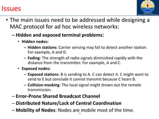
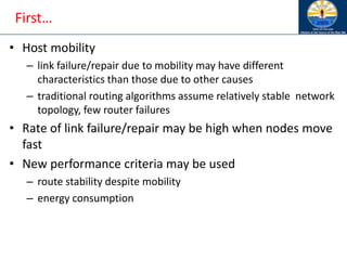
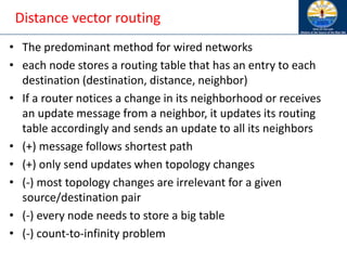
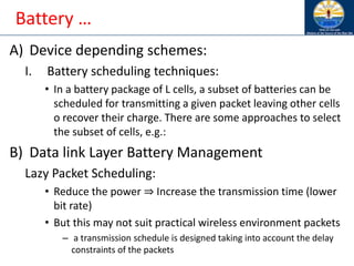
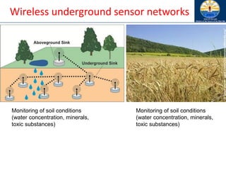
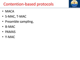
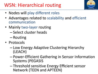
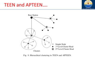
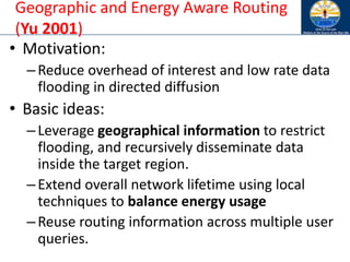
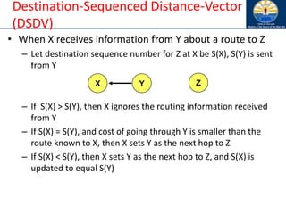
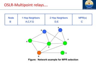
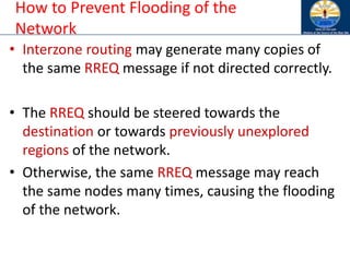
79. Destination-Sequenced Distance-Vector
(DSDV) [Perkins94Sigcomm]
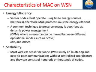
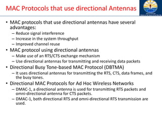
• Each node maintains a routing table which stores
– next hop, cost metric towards each destination
– a sequence number that is created by the destination itself
• Each node periodically forwards routing table to neighbors
– Each node increments and appends its sequence number when sending its
local routing table
• Each route is tagged with a sequence number; routes with greater
sequence numbers are preferred
• Each node advertises a monotonically increasing even sequence
number for itself
• When a node decides that a route is broken, it increments the
sequence number of the route and advertises it with infinite
metric
• Destination advertises new sequence number

80. Destination-Sequenced Distance-Vector
(DSDV)
• When X receives information from Y about a route to Z
– Let destination sequence number for Z at X be S(X), S(Y) is sent
from Y
– If S(X) > S(Y), then X ignores the routing information received
from Y
– If S(X) = S(Y), and cost of going through Y is smaller than the
route known to X, then X sets Y as the next hop to Z
– If S(X) < S(Y), then X sets Y as the next hop to Z, and S(X) is
updated to equal S(Y)
X Y Z

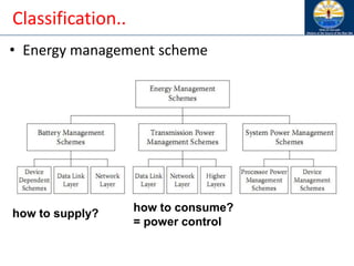
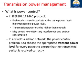
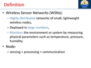
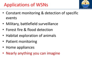
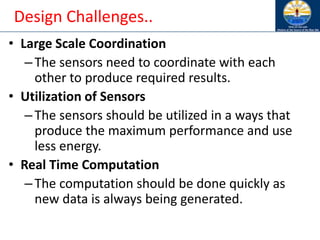
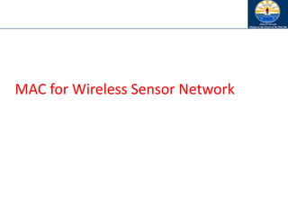
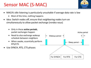
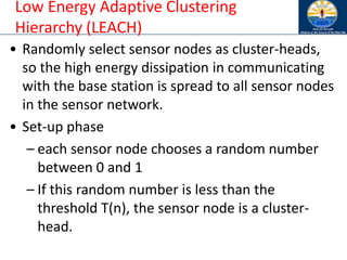
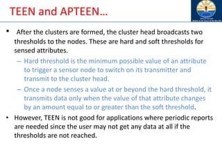
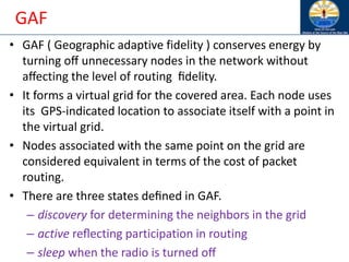
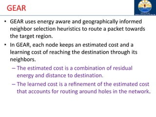
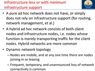
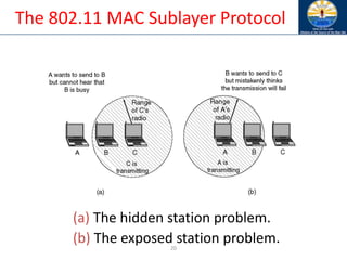
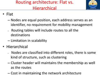
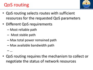
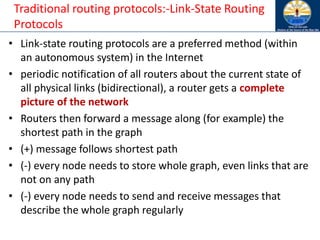
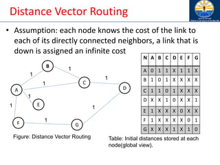
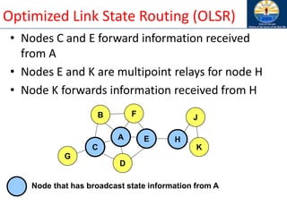
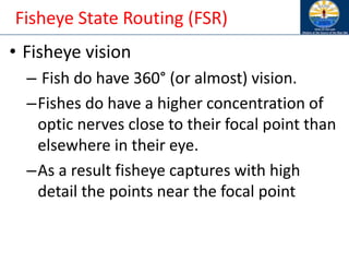
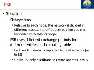
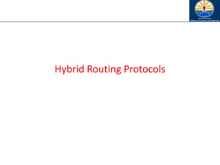
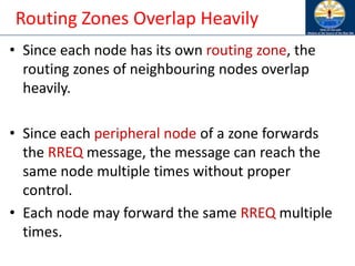
81. Optimized Link State Routing (OLSR)
[Jacquet00ietf]
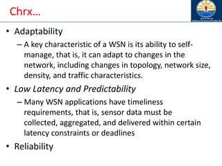
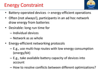
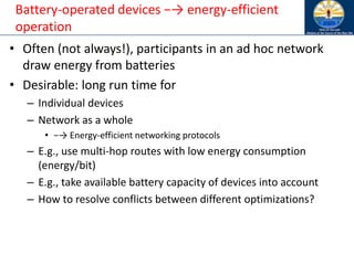
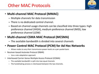
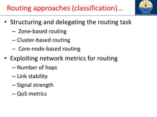
• Nodes C and E are multipoint relays of node A
– Multipoint relays of A are its neighbors such that each two-
hop neighbor of A is a one-hop neighbor of one multipoint
relay of A
– Nodes exchange neighbor lists to know their 2-hop neighbors
and choose the multipoint relays
A
B F
C
D
E H
G
K
J
Node that has broadcast state information from A

82. Optimized Link State Routing (OLSR)
• Nodes C and E forward information received
from A
• Nodes E and K are multipoint relays for node H
• Node K forwards information received from H
A
B F
C
D
E H
G
K
J
Node that has broadcast state information from A

83. OSLR….
• OLSR
– Inherits Stability of Link-state protocol
– Selective Flooding
– only MPR retransmit control messages:
• Minimize flooding
– Suitable for large and dense networks

84. OSLR-Multipoint relays
• MPRs = Set of selected neighbor nodes
• Minimize the flooding of broadcast packets
• Each node selects its MPRs among its on hop neighbors
– The set covers all the nodes that are two hops away
• MPR Selector = a node which has selected node as MPR
• The information required to calculate the multipoint relays :
– The set of one-hop neighbors and the two-hop neighbors
• Set of MPRs is able to transmit to all two-hop neighbors
• Link between node and it’s MPR is bidirectional.

85. OSLR-Multipoint relays….
• To obtain the information about one-hop neighbors :
– Use HELLO message (received by all one-hop neighbors)
• To obtain the information about two-hop neighbors :
– Each node attaches the list of its own neighbors
• Once a node has its one and two-hop neighbor sets :
– Can select a MPRs which covers all its two-hop neighbors

86. OSLR-Multipoint relays….
Node 1 Hop Neighbors 2 Hop Neighbors MPR(s)
B A,C,F,G D,E C
A
B
C
D
E
F
G
Figure: Network example for MPR selection

87. Fisheye State Routing (FSR)
• Fisheye vision
– Fish do have 360° (or almost) vision.
–Fishes do have a higher concentration of
optic nerves close to their focal point than
elsewhere in their eye.
–As a result fisheye captures with high
detail the points near the focal point

88. FSR
• Observation and problem
– When destination is far away, details about path are
not relevant – only in vicinity are details required
– reducing control traffic at the expense of routing table
accuracy
• Motivation
– Look at the graph as if through a fisheye lens, to
reduce the size of the routing update messages
– Regions of different accuracy of routing information
• Solution
– Fisheye State Routing

89. FSR
• Solution
–Fisheye lens
• Relative to each node, the network is divided in
different scopes, more frequent routing updates
for nodes with smaller scope
–FSR uses different exchange periods for
different entries in the routing table
• Each node maintains topology table of network (as
in LS)
• Unlike LS: only distribute link state updates locally.

90. Scope of FSR

91. FSR
• Routing update frequency decreases with distance to
destination
• Higher frequency updates within a close zone and lower
frequency updates to a remote zone
• Highly accurate routing information about the
immediate neighborhood of a node; progressively less
detail for areas further away from the node
• Major scalability benefit
– control traffic decreases significantly
• Unsolved problems
– Route table size still grows linearly with network size
– Out of date routes to remote destinations

92. Summary of proactive routing
• Table-Driven Routing Protocol:
–continuously evaluate the routes
–attempt to maintain consistent, up-to-date
routing information
• when a route is needed, one may be ready
immediately
–when the network topology changes
• the protocol responds by propagating updates
throughout the network to maintain a consistent
view

93. Reactive Routing Protocols

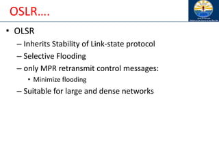
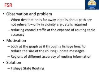
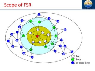
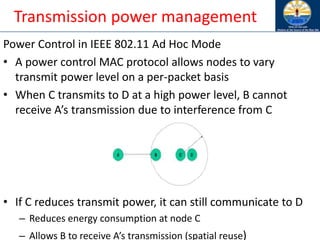
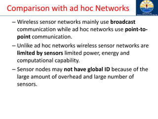
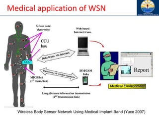
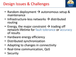
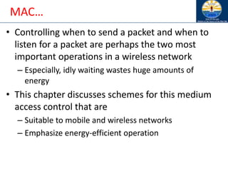
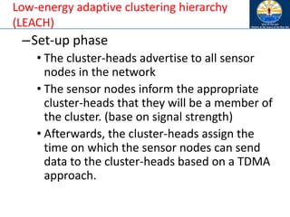
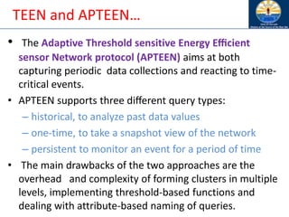
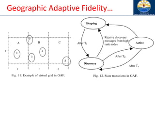
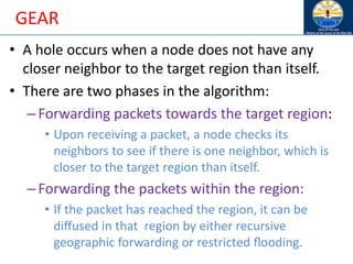
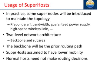
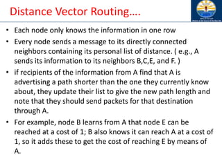
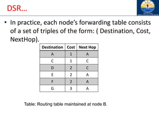
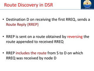
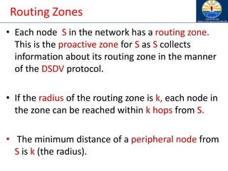
94. Dynamic Source Routing (DSR)
[Johnson96]
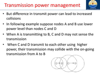
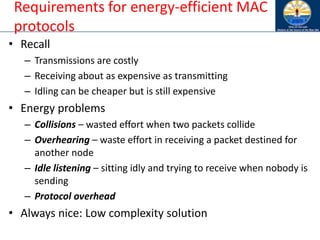
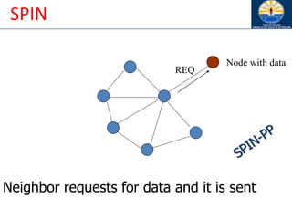
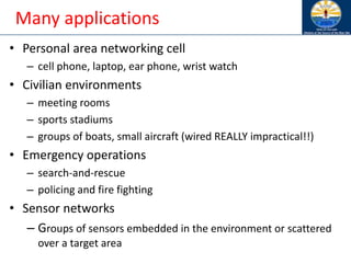
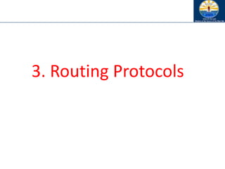
• When node S wants to send a packet to node D,
but does not know a route to D, node S initiates a
route discovery
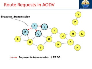
• Source node S floods Route Request (RREQ)
• Each node appends own identifier when
forwarding RREQ

95. Route Discovery in DSR
B
A
S E
F
H
J
D
C
G
I
K
Z
Y
Represents a node that has received RREQ for D from S
M
N
L

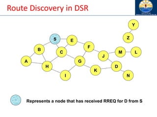
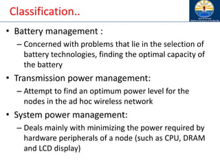
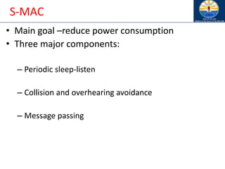
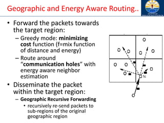
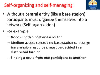
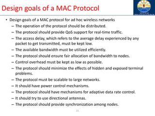
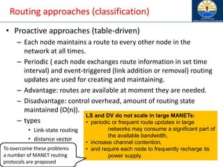
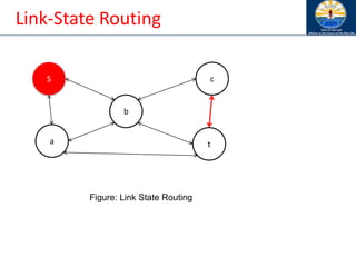
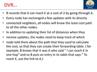
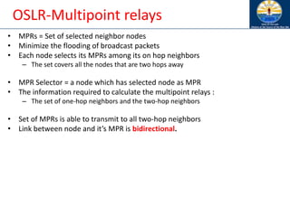
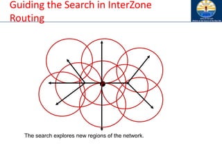
96. Route Discovery in DSR
B
A
S
E
F
H
J
D
C
G
I
K
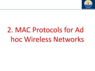
Represents transmission of RREQ
Z
Y
Broadcast transmission
M
N
L
[S]
[X,Y] Represents list of identifiers appended to RREQ

97. Route Discovery in DSR
B
A
S E
F
H
J
D
C
G
I
K
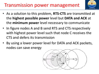
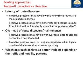
• Node H receives packet RREQ from two neighbors:
potential for collision
Z
Y
M
N
L
[S,E]
[S,C]

98. Route Discovery in DSR
B
A
S E
F
H
J
D
C
G
I
K
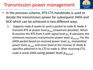
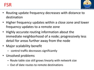
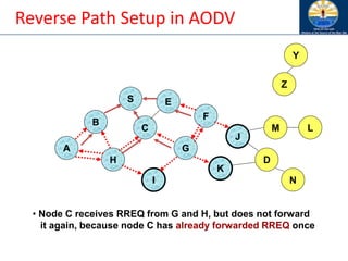
• Node C receives RREQ from G and H, but does not forward
it again, because node C has already forwarded RREQ once
Z
Y
M
N
L
[S,C,G]
[S,E,F]

99. Route Discovery in DSR
B
A
S E
F
H
J
D
C
G
I
K
Z
Y
M
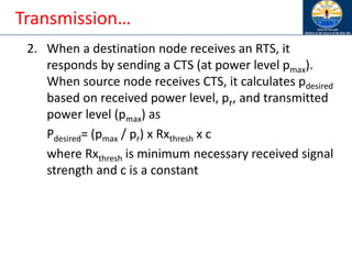
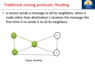
• Nodes J and K both broadcast RREQ to node D
• Since nodes J and K are hidden from each other, their
transmissions may collide
N
L
[S,C,G,K]
[S,E,F,J]

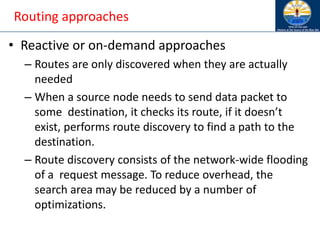
100. Route Discovery in DSR
B
A
S E
F
H
J
D
C
G
I
K
Z
Y
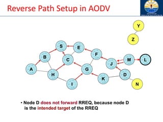
• Node D does not forward RREQ, because node D
is the intended target of the route discovery
M
N
L
[S,E,F,J,M]

101. Route Discovery in DSR
• Destination D on receiving the first RREQ, sends a
Route Reply (RREP)
• RREP is sent on a route obtained by reversing the
route appended to received RREQ
• RREP includes the route from S to D on which
RREQ was received by node D

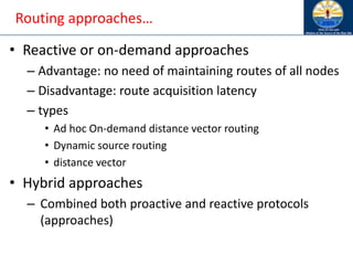
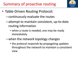
102. Route Reply in DSR
B
A
S E
F
H
J
D
C
G
I
K
Z
Y
M
N
L
RREP [S,E,F,J,D]
Represents RREP control message

103. Dynamic Source Routing (DSR)
• Node S on receiving RREP, caches the route
included in the RREP
• When node S sends a data packet to D, the entire
route is included in the packet header
– hence the name source routing
• Intermediate nodes use the source route
included in a packet to determine to whom a
packet should be forwarded

104. Data Delivery in DSR
B
A
S E
F
H
J
D
C
G
I
K
Z
Y
M
N
L
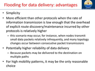
DATA [S,E,F,J,D]
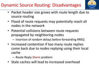
Packet header size grows with route length

105. DSR Optimization: Route Caching
• Each node caches a new route it learns by any means
• When node S finds route [S,E,F,J,D] to node D, node S
also learns route [S,E,F] to node F
• When node K receives Route Request [S,C,G] destined
for node, node K learns route [K,G,C,S] to node S
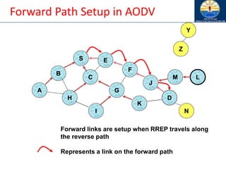
• When node F forwards Route Reply RREP [S,E,F,J,D],
node F learns route [F,J,D] to node D
• When node E forwards Data [S,E,F,J,D] it learns route
[E,F,J,D] to node D
• A node may also learn a route when it overhears Data
• Problem: Stale caches may increase overheads

106. Dynamic Source Routing: Advantages
• Routes maintained only between nodes who
need to communicate
– reduces overhead of route maintenance
• Route caching can further reduce route discovery
overhead
• A single route discovery may yield many routes to
the destination, due to intermediate nodes
replying from local caches

107. Dynamic Source Routing: Disadvantages
• Packet header size grows with route length due to
source routing
• Flood of route requests may potentially reach all
nodes in the network
• Potential collisions between route requests
propagated by neighboring nodes
– insertion of random delays before forwarding RREQ
• Increased contention if too many route replies
come back due to nodes replying using their local
cache
– Route Reply Storm problem
• Stale caches will lead to increased overhead

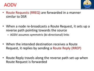
108. Ad Hoc On-Demand Distance Vector
Routing (AODV) [Perkins99Wmcsa]
• DSR includes source routes in packet headers
• Resulting large headers can sometimes degrade
performance
– particularly when data contents of a packet are small
• AODV attempts to improve on DSR by maintaining
routing tables at the nodes, so that data packets do not
have to contain routes
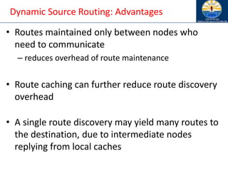
• AODV retains the desirable feature of DSR that routes
are maintained only between nodes which need to
communicate

109. AODV
• Route Requests (RREQ) are forwarded in a manner
similar to DSR
• When a node re-broadcasts a Route Request, it sets up a
reverse path pointing towards the source
– AODV assumes symmetric (bi-directional) links
• When the intended destination receives a Route
Request, it replies by sending a Route Reply (RREP)
• Route Reply travels along the reverse path set-up when
Route Request is forwarded

110. Route Requests in AODV
B
A
S E
F
H
J
D
C
G
I
K
Z
Y
Represents a node that has received RREQ for D from S
M
N
L

111. Route Requests in AODV
B
A
S E
F
H
J
D
C
G
I
K
Represents transmission of RREQ
Z
Y
Broadcast transmission
M
N
L

112. Route Requests in AODV
B
A
S E
F
H
J
D
C
G
I
K
Represents links on Reverse Path
Z
Y
M
N
L

113. Reverse Path Setup in AODV
B
A
S E
F
H
J
D
C
G
I
K
• Node C receives RREQ from G and H, but does not forward
it again, because node C has already forwarded RREQ once
Z
Y
M
N
L

114. Reverse Path Setup in AODV
B
A
S E
F
H
J
D
C
G
I
K
Z
Y
M
N
L

115. Reverse Path Setup in AODV
B
A
S E
F
H
J
D
C
G
I
K
Z
Y
• Node D does not forward RREQ, because node D
is the intended target of the RREQ
M
N
L

116. Forward Path Setup in AODV
B
A
S E
F
H
J
D
C
G
I
K
Z
Y
M
N
L
Forward links are setup when RREP travels along
the reverse path
Represents a link on the forward path

117. Route Request and Route Reply
• Route Request (RREQ) includes the last known sequence number for the
destination
• An intermediate node may also send a Route Reply (RREP) provided that it
knows a more recent path than the one previously known to sender
• Intermediate nodes that forward the RREP, also record the next hop to
destination
• A routing table entry maintaining a reverse path is purged after a timeout
interval
• A routing table entry maintaining a forward path is purged if not used for a
active_route_timeout interval

118. Link Failure
• A neighbor of node X is considered active for a routing table entry if the
neighbor sent a packet within active_route_timeout interval which was
forwarded using that entry
• Neighboring nodes periodically exchange hello message
• When the next hop link in a routing table entry breaks, all active neighbors are
informed
• Link failures are propagated by means of Route Error (RERR) messages, which
also update destination sequence numbers

119. Route Error
• When node X is unable to forward packet P (from node S to node D) on link
(X,Y), it generates a RERR message
• Node X increments the destination sequence number for D cached at node X
• The incremented sequence number N is included in the RERR
• When node S receives the RERR, it initiates a new route discovery for D using
destination sequence number at least as large as N
• When node D receives the route request with destination sequence number N,
node D will set its sequence number to N, unless it is already larger than N

120. AODV: Summary
• Routes need not be included in packet headers
• Nodes maintain routing tables containing entries only for
routes that are in active use
• At most one next-hop per destination maintained at
each node
– DSR may maintain several routes for a single destination
• Sequence numbers are used to avoid old/broken routes
• Sequence numbers prevent formation of routing loops
• Unused routes expire even if topology does not change

121. Hybrid Routing Protocols

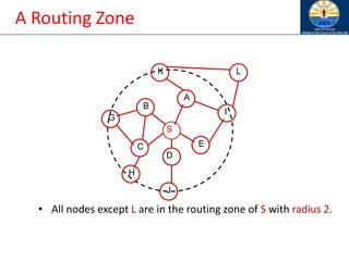
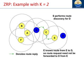
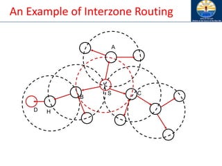
122. Zone Routing Protocol (ZRP) [Haas98]
• ZRP combines proactive and reactive approaches
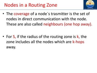
• All nodes within hop distance at most d from a node X
are said to be in the routing zone of node X
• All nodes at hop distance exactly d are said to be
peripheral nodes of node X’s routing zone
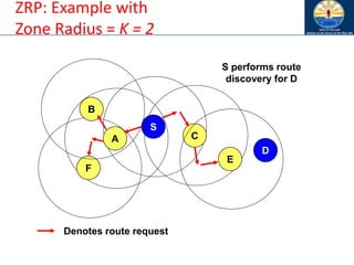
• Intra-zone routing: Proactively maintain routes to all
nodes within the source node’s own zone.
• Inter-zone routing: Use an on-demand protocol (similar
to DSR or AODV) to determine routes to outside zone.
Zone Routing Protocol (ZRP), Nicklas Beijar

123. Routing Zones
• Each node S in the network has a routing zone.
This is the proactive zone for S as S collects
information about its routing zone in the manner
of the DSDV protocol.
• If the radius of the routing zone is k, each node in
the zone can be reached within k hops from S.
• The minimum distance of a peripheral node from
S is k (the radius).

124. A Routing Zone
S
L
K
G
H
I
J
A
B
C
D
E
• All nodes except L are in the routing zone of S with radius 2.

125. Nodes in a Routing Zone
• The coverage of a node´s trasmitter is the set of
nodes in direct communication with the node.
These are also called neighbours (one hop away).
• For S, if the radius of the routing zone is k, the
zone includes all the nodes which are k-hops
away.

126. Neighbour Discovery Protocol
• Like other ad hoc routing protocols, each node
executes ZRP to know its current neighbours.
• Each node transmits a hello message at regular
intervals to all nodes within its transmission
range.
• If a node P does not receive a hello message from
a previously known neighbour Q, P removes Q
from its list of neighbours.

127. ZRP: Example with
Zone Radius = K = 2
S
C
A
E
F
B
D
S performs route
discovery for D
Denotes route request

128. ZRP: Example with K = 2
S
C
A
E
F
B
D
S performs route
discovery for D
Denotes route reply
E knows route from E to D,
so route request need not be
forwarded to D from E

129. ZRP: Example with K = 2
S
C
A
E
F
B
D
S performs route
discovery for D
Denotes route taken by Data

130. Interzone Routing
• The interzone routing discovers routes to the
destination reactively.
• Consider a source (S) and a destination (D). If D is
within the routing zone of S, the routing is
completed in the intrazone routing phase.
• Otherwise, S sends the packet to the peripheral
nodes of its zone through bordercasting.

131. Bordercasting
• The bordercasting to peripheral nodes can be
done mainly in two ways :
– By maintaining a multicast tree for the peripheral
nodes. S is the root of this tree.
– Otherwise, S maintains complete routing table for its
zone and routes the packet to the peripheral nodes by
consulting this routing table.

132. Interzone Route Discovery
• S sends a route request (RREQ) message to the
peripheral nodes of its zone through
bordercasting.
• Each peripheral node P executes the same
algorithm.
– First, P checks whether the destination D is within its
routing zone and if so, sends the packet to D.
– Otherwise, P sends the packet to the peripheral nodes
of its routing zone through bordercasting.

133. An Example of Interzone Routing
S
D
B
H
A
C

134. Route Reply in Interzone Routing
• If a node P finds that the destination D is within
its routing zone, P can initiate a route reply.
• Each node appends its address to the RREQ
message during the route request phase. This is
similar to route request phase in DSR.
• This accumulated address can be used to send
the route reply (RREP) back to the source node S.

135. Route Reply in Interzone Routing
• An alternative strategy is to keep forward and
backward links at every node´s routing table
similar to the AODV protocol. This helps in
keeping the packet size constant.
• A RREQ usually results in more than one RREP
and ZRP keeps track of more than one path
between S and D. An alternative path is chosen in
case one path is broken.

136. Route Maintenance
• When there is a broken link along an active
path between S and D, a local path repair
procedure is initiated.
• A broken link is always within the routing zone
of some node.
A
B

137. Route Maintenance
• Hence, repairing a broken link requires
establishing a new path between two nodes
within a routing zone.
• The repair is done by the starting node of the link
(node A in the previous diagram) by sending a
route repair message to node B within its routing
zone.
• This is like a RREQ message from A with B as the
destination.

138. How to Prevent Flooding of the
Network
• Interzone routing may generate many copies of
the same RREQ message if not directed correctly.
• The RREQ should be steered towards the
destination or towards previously unexplored
regions of the network.
• Otherwise, the same RREQ message may reach
the same nodes many times, causing the flooding
of the network.

139. Routing Zones Overlap Heavily
• Since each node has its own routing zone, the
routing zones of neighbouring nodes overlap
heavily.
• Since each peripheral node of a zone forwards
the RREQ message, the message can reach the
same node multiple times without proper
control.
• Each node may forward the same RREQ multiple
times.

140. Guiding the Search in InterZone
Routing
The search explores new regions of the network.

141. Routing Summary
• Protocols
– Typically divided into proactive, reactive and hybrid
– Plenty of routing protocols. Discussion here is far from exhaustive
• Performance Studies
– Typically studied by simulations using ns, discrete event simulator
– Nodes (10-30) remains stationary for pause time seconds (0-900s)
and then move to a random destination (1500m X300m space) at
a uniform speed (0-20m/s). CBR traffic sources (4-30 packets/sec,
64-1024 bytes/packet)
– Attempt to estimate latency of route discovery, routing overhead
…
• Actual trade-off depends a lot on traffic and mobility
patterns
– Higher traffic diversity (more source-destination pairs) increases
overhead in on-demand protocols
– Higher mobility will always increase overhead in all protocols

142. Transport in MANET

143. User Datagram Protocol (UDP)
• Studies comparing different routing protocols for MANET typically
measure UDP performance
• Several performance metrics are used
– routing overhead per data packet
– packet delivery delay
– throughput/loss
• Many variables affect performance
– Traffic characteristics
– Mobility characteristics
– Node capabilities
• Difficult to identify a single scheme that will perform well in all
environments
• Several relevant studies [Broch98Mobicom, Das9ic3n,
Johansson99Mobicom, Das00Infocom, Jacquet00Inria]
On the evaluation of TCP in MANETs,

144. Transmission Control Protocol (TCP)
• Reliable ordered delivery
– Reliability achieved by means of retransmissions if necessary
• End-to-end semantics
– Receiver sends cumulative acknowledgements for in-sequence packets
– Receiver sends duplicate acknowledgements for out-of-sequence packets
• Implements congestion avoidance and control using sliding-window
– Window size is minimum of
• receiver’s advertised window - determined by available buffer space at the
receiver
• congestion window - determined by the sender, based on feedback from the
network
– Congestion window size bounds the amount of data that can be sent per round-trip
time

145. Detection of packet loss in TCP
• Retransmission timeout (RTO)
– sender sets retransmission timer for only one packet
– if Ack not received before timer expiry, the packet is assumed
lost
– RTO dynamically calculated, doubles on each timeout
• Duplicate acks
– sender assumes packet loss if it receives three consecutive
duplicate acknowledgements (dupacks)
• On detecting a packet loss, TCP sender assumes that
network congestion has occurred and drastically reduces
the congestion window

146. TCP in MANET
Several factors affect TCP performance in MANET:
• Wireless transmission errors
– may cause fast retransmit, which results in
• retransmission of lost packet
• reduction in congestion window
– reducing congestion window in response to errors is
unnecessary
• Multi-hop routes on shared wireless medium
– Longer connections are at a disadvantage compared to shorter
connections, because they have to contend for wireless
access at each hop
• Route failures due to mobility

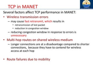
147. Impact of Multi-hop Wireless Paths
TCP throughput degrades with increase in number of hops
Packet transmission can occur on at most one hop among
three consecutive hops
– Increasing the number of hops from 1 to 2, 3 results in
increased delay, and decreased throughput
• Increasing number of hops beyond 3 allows
simultaneous transmissions on more than one link,
however, degradation continues due to contention
between TCP Data and Acks traveling in opposite
directions
• When number of hops is large enough (>6), throughput
stabilizes [Holland99]

148. mobility causes
link breakage,
resulting in route
failure
TCP data and acks
en route discarded
Impact of Node Mobility
TCP sender times out.
Starts sending packets again
Route is
repaired
No
throughput
No throughput
despite route repair
TCP throughput degrades with increase in mobility but not always
Larger route repair
delays are especially
harmful

149. Improved Throughput with Increased
Mobility
▪Low speed: (Route from A to D is broken for ~1.5 seconds)
•When TCP sender times after 1 second, route still broken.
•TCP times out after another 2 seconds, and only then resumes
▪High speed: (Route from A to D is broken for ~0.75 seconds)
•When TCP sender times out after 1 second, route is repaired
▪TCP timeout interval somewhat (not entirely) independent of speed
▪Network state at higher speed may sometimes be more favorable than
lower speed
C
B
D
A
C
B
D
A
C
B
D
A

150. Impact of Route Caching
TCP performance typically degrades when caches are used for route
repair
• When a route is broken, route discovery returns a cached route from
local cache or from a nearby node
• After a time-out, TCP sender transmits a packet on the new route.
However, typically the cached route has also broken after it was
cached
• Another route discovery, and TCP time-out interval
• Process repeats until a good route is found
timeout due
to route failure
timeout, cached
route is broken
timeout, second cached
route also broken

151. Caching and TCP performance
• Caching can result in faster route repair
– Faster does not necessarily mean correct
– If incorrect repairs occur often enough, caching performs
poorly
• If cache accuracy is not high enough, gains in routing
overhead may be offset by loss of TCP performance due
to multiple time-outs
• Need mechanisms for determining when cached routes
are stale

152. Impact of Acknowledgements
• TCP Acks (and link layer acks) share the wireless bandwidth with
TCP data packets
• Data and Acks travel in opposite directions
– In addition to bandwidth usage, acks require additional receive-send
turnarounds, which also incur time penalty
• Reduction of contention between data and acks, and frequency of
send-receive turnaround
• Mitigation [Balakrishnan97]
– Piggybacking link layer acks with data
– Sending fewer TCP acks - ack every d-th packet (d may be chosen
dynamically)
– Ack filtering - Gateway may drop an older ack in the queue, if a new ack
arrives

153. TCP Parameters after Route Repair
• Window Size after route repair
– Same as before route break: may be too optimistic
– Same as startup: may be too conservative
– Better be conservative than overly optimistic
– Reset window to small value; let TCP learn the window size
• Retransmission Timeout (RTO) after route repair
– Same as before route break: may be too small for long routes
– Same as TCP start-up: may be too large and respond slowly to
packet loss
– new RTO could be made a function of old RTO and route
lengths

154. Improving TCP Throughput
• Network feedback
– Network knows best (why packets are lost)
– Need to modify transport & network layer to receive/send
feedback
- Need mechanisms for information exchange between layers
• Inform TCP of route failure by explicit message
• Let TCP know when route is repaired
– Probing
– Explicit notification
– Better route caching mechanisms
• Reduces repeated TCP timeouts and backoff

155. Conclusion
Issues other than routing have received much less
attention
Other interesting problems:
• Applications for MANET
• Address assignment
• QoS issues
• Improving interaction between protocol layers

156. 4. Energy in MANET

157. Introduction
• In ad hoc networks the devices are battery
powered
• So the computation and communication capacity
of each device is constrained
• Devices that expend their whole energy can be
recharged when they leave the network
• Energy resources and computation workloads
have different distributions within the network
• Therefore it is beneficial to redistribute spare
energy resources to satisfy varying workloads in
the network

158. Main reason for Energy management in
ad hoc networks
• Limited Energy Reserve: The improvement in battery
technologies is very slow
• Difficulties in replacing the batteries: E.g. in battlefields
or emergency applications
• Lack of central coordination: In ad hoc networks as
distributed networks some nodes may work as relay
nodes; when relay traffic is heavy the power
consumption is high
• Constraints on the battery source: The batteries should
be small and not heavy; So low power is available at
each node
• Selection of optimal transmission power: Higher
transmission power results in high

159. Classification..
• Energy management scheme
how to supply?
how to consume?
= power control

160. Classification..
• Battery management :
– Concerned with problems that lie in the selection of
battery technologies, finding the optimal capacity of
the battery
• Transmission power management:
– Attempt to find an optimum power level for the
nodes in the ad hoc wireless network
• System power management:
– Deals mainly with minimizing the power required by
hardware peripherals of a node (such as CPU, DRAM
and LCD display)

161. Battery Management Schemes
• The lifetime of a node is determined by the
capacity of its energy source and the energy
required by the node.
• There are some device dependent approaches
that increase the battery lifetime by exploiting its
internal characteristics.
• Key Fact: Batteries recover their charge when idle
– Use some batteries and leave others to idle/recover

162. Battery …
A) Device depending schemes:
I. Battery scheduling techniques:
• In a battery package of L cells, a subset of batteries can be
scheduled for transmitting a given packet leaving other cells
o recover their charge. There are some approaches to select
the subset of cells, e.g.:
B) Data link Layer Battery Management
Lazy Packet Scheduling:
• Reduce the power ⇒ Increase the transmission time (lower
bit rate)
• But this may not suit practical wireless environment packets
– a transmission schedule is designed taking into account the delay
constraints of the packets

163. Transmission power management
• What is power control?
– In IEEE802.11 MAC protocol:
• Each node transmits packets at the same power level:
maximal possible power level.
• Transmission power may be higher than enough
• May generate unnecessary interference and energy
consumption
– In a wireless ad hoc network, the power control
problem is to choose the appropriate transmit power
level for every packet to ensure that the transmitted
packet is received correctly.

164. Transmission power management
Power Control in IEEE 802.11 Ad Hoc Mode
• A power control MAC protocol allows nodes to vary
transmit power level on a per-packet basis
• When C transmits to D at a high power level, B cannot
receive A’s transmission due to interference from C
• If C reduces transmit power, it can still communicate to D
– Reduces energy consumption at node C
– Allows B to receive A’s transmission (spatial reuse)

165. Transmission power management
• But difference in transmit power can lead to increased
collisions
• In following example suppose nodes A and B use lower
power level than nodes C and D
• When A is transmitting to B, C and D may not sense the
transmission
• When C and D transmit to each other using higher
power, their transmission may collide with the on-going
transmission from A to B

166. Transmission power management
• As a solution to this problem, RTS-CTS are transmitted at
the highest possible power level but DATA and ACK at
the minimum power level necessary to communicate
• In figure nodes A and B send RTS and CTS respectively
with highest power level such that node C receives the
CTS and defers its transmission
• By using a lower power level for DATA and ACK packets,
nodes can save energy

167. Transmission power management
• In the previous scheme, RTS-CTS handshake is used to
decide the transmission power for subsequent DATA and
ACK which can be achieved in two different ways
1. Suppose node A wants to send a packet to node B. Node A
transmit RTS at power level pmax (maximum possible). When
B receives the RTS from A with signal level pr, B calculates the
minimum necessary transmission power level, pdesired. For the
DATA packet based on received power level, pr, transmitted
power level, pmax, and noise level at the receiver B. Node B
specifies pdesired in its CTS to node A. After receiving CTS,
node A sends DATA using power level pdesired.

168. Transmission…
2. When a destination node receives an RTS, it
responds by sending a CTS (at power level pmax).
When source node receives CTS, it calculates pdesired
based on received power level, pr, and transmitted
power level (pmax) as
Pdesired= (pmax / pr) x Rxthresh x c
where Rxthresh is minimum necessary received signal
strength and c is a constant

169. System power management scheme
• Efficient design of the hardware brings about
significant reduction in the power consumed.
• This can be effected by operating some of the
peripheral devices in power-saving mode by
turning them off under idle conditions.
• System power consists of the power used by all
hardware units of the node. This power can be
conserved significantly by applying the following
schemes:
– Processor power management schemes
– Device power management schemes

170. Summary
• Power control is important in wireless ad hoc
networks for at least two reasons:
(i) It can impact on battery life
(ii) It can impact on the traffic carrying capacity of
the network.

172. 9. Wireless Sensor Networks

173. Definition
• Wireless Sensor Networks (WSNs):
– Highly distributed networks of small, lightweight
wireless nodes,
– Deployed in large numbers,
– Monitors the environment or system by measuring
physical parameters such as temperature, pressure,
humidity.
• Node:
– sensing + processing + communication

174. Comparison with ad hoc Networks
– Wireless sensor networks mainly use broadcast
communication while ad hoc networks use point-to-
point communication.
– Unlike ad hoc networks wireless sensor networks are
limited by sensors limited power, energy and
computational capability.
– Sensor nodes may not have global ID because of the
large amount of overhead and large number of
sensors.

175. Characteristics of Wireless Sensor
Networks
• Wireless Sensor Networks mainly consists of
sensors. Sensors are -
–low power
–limited memory
–energy constrained due to their small size.
• Wireless networks can also be deployed in
extreme environmental conditions and may be
prone to enemy attacks.
• Although deployed in an ad hoc manner they
need to be self organized and self healing and
can face constant reconfiguration.

176. Chrx…
• Heterogeneity
–The devices deployed maybe of various types
and need to collaborate with each other.
• Distributed Processing
–The algorithms need to be centralized as the
processing is carried out on different nodes.
• Low Bandwidth Communication
–The data should be transferred efficiently
between sensors

177. Applications of WSNs
• Constant monitoring & detection of specific
events
• Military, battlefield surveillance
• Forest fire & flood detection
• Habitat exploration of animals
• Patient monitoring
• Home appliances
• Nearly anything you can imagine

178. Medical application of WSN
Wireless Body Sensor Network Using Medical Implant Band (Yuce 2007)

179. Environmental Monitoring..
Zebranet: a WSN to study the behavior of
zebras
• Special GPS-equipped collars were attached to zebras
• Data exchanged with peer-to-peer info swaps
• Coming across a few zebras gives access to the data

180. Wireless underground sensor networks
Monitoring of soil conditions
(water concentration, minerals,
toxic substances)
Monitoring of soil conditions
(water concentration, minerals,
toxic substances)

181. Design Challenges..
• Large Scale Coordination
–The sensors need to coordinate with each
other to produce required results.
• Utilization of Sensors
–The sensors should be utilized in a ways that
produce the maximum performance and use
less energy.
• Real Time Computation
–The computation should be done quickly as
new data is always being generated.

182. Design Issues & Challenges
• Random deployment → autonomous setup &
maintenance
• Infrastructure-less networks → distributed
routing
• Energy, the major constraint → trading off
network lifetime for fault tolerance or accuracy
of results
• Hardware energy efficiency
• Distributed synchronization
• Adapting to changes in connectivity
• Real-time communication, QoS
• Security

183. Operational Challenges
• Energy Efficiency
• Limited storage and computation
• Low bandwidth and high error rates
• Errors are common
–Wireless communication
–Noisy measurements
–Node failure are expected
• Scalability to a large number of sensor nodes
• Survivability in harsh environments
• Experiments are time- and space-intensive

184. Enabling Technologies
Embedded
Networked
Sensing
Control system w/
Small form factor
Untethered nodes
Exploit
collaborative
Sensing, action
Tightly coupled to physical world
Embed numerous distributed
devices to monitor and interact
with physical world
Network devices to coordinate
and perform higher-level tasks
Exploit spatially and temporally dense, in situ, sensing and actuation

185. MAC for Wireless Sensor Network

186. MAC…
• Controlling when to send a packet and when to
listen for a packet are perhaps the two most
important operations in a wireless network
– Especially, idly waiting wastes huge amounts of
energy
• This chapter discusses schemes for this medium
access control that are
– Suitable to mobile and wireless networks
– Emphasize energy-efficient operation

187. Principal options and difficulties
• Medium access in wireless networks is difficult mainly
because of
– Impossible (or very difficult) to sende and receive at the same
time
– Interference situation at receiver is what counts for
transmission success, but can be very different from what
sender can observe
– High error rates (for signaling packets) compound the issues
• Requirement
– As usual: high throughput, low overhead, low error rates, …
– Additionally: energy-efficient, handle switched off devices!

188. Characteristics of MAC on WSN
• Energy Efficiency
– Sensor nodes must operate using finite energy sources
(batteries), therefore MAC protocols must be energy-efficient
– A common technique to preserve energy is described as
dynamic power management
(DPM), where a resource can be moved between different
operational modes such as active,
idle, and asleep
• Scalability
– Most wireless sensor networks (WSNs) rely on multi-hop and
peer-to-peer communications without centralized coordinators
and they can consist of hundreds or thousands of nodes.

189. Chrx…
• Adaptability
– A key characteristic of a WSN is its ability to self-
manage, that is, it can adapt to changes in the
network, including changes in topology, network size,
density, and traffic characteristics.
• Low Latency and Predictability
– Many WSN applications have timeliness
requirements, that is, sensor data must be
collected, aggregated, and delivered within certain
latency constraints or deadlines
• Reliability

190. Requirements for energy-efficient MAC
protocols
• Recall
– Transmissions are costly
– Receiving about as expensive as transmitting
– Idling can be cheaper but is still expensive
• Energy problems
– Collisions – wasted effort when two packets collide
– Overhearing – waste effort in receiving a packet destined for
another node
– Idle listening – sitting idly and trying to receive when nobody is
sending
– Protocol overhead
• Always nice: Low complexity solution

191. Overview
Wireless medium access
Centralized
Distributed
Contention-
based
Schedule-
based
Fixed
assignment
Demand
assignment
Contention-
based
Schedule-
based
Fixed
assignment
Demand
assignment

192. Contention-based protocols
• MACA
• S-MAC, T-MAC
• Preamble sampling,
• B-MAC
• PAMAS
• Y-MAC

193. Sensor MAC (S-MAC)
• MACA’s idle listening is particularly unsuitable if average data rate is low
• Most of the time, nothing happens
• Idea: Switch nodes off, ensure that neighboring nodes turn on
simultaneously to allow packet exchange (rendez-vous)
• Only in these active periods,
packet exchanges happen
• Need to also exchange wakeup
schedule between neighbors
• When awake, essentially perform
RTS/CTS
• Use SYNCH, RTS, CTS phases
Wakeup period
Active period
Sleep period
For SYNCH For RTS For CTS

194. S-MAC
• Main goal –reduce power consumption
• Three major components:
– Periodic sleep-listen
– Collision and overhearing avoidance
– Message passing

195. Periodic Sleep-Listen
◼ Each node goes to sleep for some time,
and then wakes up and listens to see if any
other node wants to talk to it.
◼ During Sleep it turn off its radio.

196. Collision and Overhearing Avoidance
• Interfering nodes go to sleep after they hear an
RTS or CTS packet.
• Duration field in each transmitted packet
indicates how long the remaining transmission
will be.

197. S-MAC synchronized islands
• Nodes try to pick up schedule synchronization from neighboring
nodes
• If no neighbor found, nodes pick some schedule to start with
• If additional nodes join, some node might learn about two
different schedules from different nodes
• “Synchronized islands”
• To bridge this gap, it has to follow both schemes
Time
A A A A
C C C C
A
B B B B
D D D
A
C
B
D
E E E
E E E
E

198. Schedule Establishment
• Node listens for certain amount of time.
• If it does not hear a schedule, it chooses a time to
sleep and broadcast this information
immediately.
• This node is called the ‘Synchornizer’.
• If a node receives a schedule before establishing
its schedule, it just follows the received schedule.
• If a node receives a different schedule, after it has
established its schedule, it listens for both the
schedules

199. Timeout MAC(T-MAC)
• In S-MAC, active period is of constant
length
• What if no traffic actually happens?
• Nodes stay awake needlessly long
• Idea: Prematurely go back to sleep
mode when no traffic has happened
for a certain time (=timeout) ! T-MAC
• Adaptive duty cycle!
• One ensuing problem: Early sleeping
• C wants to send to D, but is
hindered by transmission A! B
• Two solutions exist – homework!
A B C D
CTS
May not
send
Timeout,
go back to
sleep as
nothing
happened

200. WiseMAC (Preamble Sampling)
• All nodes defined to have two communication
channels.
• Data channel uses TDMA
• Control channel uses CSMA
• Preamble sampling used to decrease idle listening
time.
• Nodes sample the medium periodically to see if
any data is going to arrive.

201. Preamble Sampling
Start transmission:
Long preamble Actual packet
Check
channel
Check
channel
Check
channel
Check
channel
• So far: Periodic sleeping supported by some means to
synchronize wake up of nodes to ensure rendez-vous
between sender and receiver
• Alternative option: Don’t try to explicitly synchronize nodes
• Have receiver sleep and only periodically sample the channel
• Use long preambles to ensure that receiver stays awake
to catch actual packet
• Example: WiseMAC

202. B-MAC - Berkeley MAC
• Combines several of the above discussed ideas
– Takes care to provide practically relevant solutions
• Clear Channel Assessment
– Adapts to noise floor by sampling channel when it is assumed
to be free
– Samples are exponentially averaged, result used in gain control
– For actual assessment when sending a packet, look at five
channel samples – channel is free if even a single one of them
is significantly below noise
– Optional: random backoff if channel is found busy
• Optional: Immediate link layer acknowledgements for
received packets

203. B-MAC II
• Low Power Listening (= preamble sampling)
– Uses the clear channel assessment techniques to decide
whether there is a packet arriving when node wakes up
– Timeout puts node back to sleep if no packet arrived
• B-MAC does not have
– Synchronization
– RTS/CTS
– Results in simpler, leaner implementation
– Clean and simple interface
• Currently: Often considered as the default WSN MAC
protocol

204. Power Aware Multiaccess with
Signaling – PAMAS
• Idea: combine busy tone with RTS/CTS
• Results in detailed overhearing avoidance, does not address idle listening
• Uses separate data and control channels
• Procedure
• Node A transmits RTS on control channel, does not sense channel
• Node B receives RTS, sends CTS on control channel if it can receive and
does not know about ongoing transmissions
• B sends busy tone as it starts to receive data
Time
Control
channel
Data
channel
RTS
A ! B
CTS
B ! A
Data
A ! B
Busy tone
sent by B

205. PAMAS – Already ongoing transmission
• Suppose a node C in vicinity of A is already receiving a packet
when A initiates RTS
• Procedure
• A sends RTS to B
• C is sending busy tone (as it receives data)
• CTS and busy tone collide, A receives no CTS, does not send data
A
B
C
?
Time
Control
channel
Data
channel
RTS
A ! B
CTS
B ! A
No data!
Busy tone by C
Similarly: Ongoing
transmission near B
destroys RTS by
busy tone

206. Traffic-Adaptive Medium Access(TRAMA)
• Aims to increase the network throughput and
energy-efficiency
• It uses a distributed election scheme based on information about
the traffic at each node to determine when nodes are allowed to
transmit.
• Helps to avoid assigning slots to nodes with no traffic to send and
to determine when nodes become idle.
• TRAMA divides time into periodic random access intervals
(signaling slots) and scheduled-access intervals (transmission
slots)
• During random-access intervals, the Neighbor Protocol (NP) is
used to propagate one-hop neighbor information among
neighboring nodes, allowing them to obtain consistent two-hop
topology information.

207. TRAMA
• Schedule Exchange Protocol (SEP), is used to
establish and broadcast actual schedules, that is,
allocations of slots to a node
• Each node computes a duration
SCHEDULE_INTERVAL, which represents the
number of slots for which the node can announce
its schedule to its neighbors.
• TRAMA reduces the probability of collisions and
increases the sleep time (and energy savings)
compared to CSMA-based protocols.

208. Y-MAC
• Similar to TDMA, Y-MAC divides time into frames
and slots, where each frame contains a broadcast
period and a unicast period.
• Every node must wake up at the beginning of a
broadcast period and nodes contend to access
the medium during this period.
• If there are no incoming broadcast messages,
each node turns off its radio awaiting its first
assigned slot in the unicast period.
• Each slot in the unicast period is assigned to
only one node for receiving data.

209. Y-MAC
• Y-MAC uses recover model
– Can be energy efficient under light traffic conditions,
because each node samples the medium only in its
own time slot
– Particularly important for radio transceivers , where
the energy costs for receiving is higher than that of
transmitting (error correction)

210. Y-MAC..
• Medium access in Y-MAC is based on synchronous low
power listening!
• The contention window (at beginning of each slot) resolves
contention between multiple senders!
• A node wishing to send data sets a random wait time (back-
off value) within the contention window!
• After this wait time, the node wakes up and senses the
medium for activity for a certain amount of time!
– if the medium is free, the node sends a preamble until
the end of the contention window to suppress competing
transmissions and the receiver wakes up at the end of the
contention window to wait for packets in its assigned slot!
– if the medium receives no signal from any of its
neighboring nodes, it turns off the radio and returns to the
sleep mode!

211. Routing Protocols in WSN

212. Introduction
• Routing in sensor networks is very challenging due to
several characteristics that distinguish them from
contemporary communication and wireless ad hoc
networks.
– First of all, it is not possible to build a global
addressing scheme for the deployment of sheer
number of sensor nodes.
– Second, in contrary to typical communication
networks almost all applications of sensor networks
require the flow of sensed data from multiple
regions (sources) to a particular sink (command
center).

213. Introduction….
– Third, generated data traffic has significant
redundancy in it since multiple sensors may generate
same data within the vicinity of a phenomenon.
– Fourth, sensor nodes are tightly constrained in terms
of transmission power, on-board energy, processing
capacity and storage and thus require careful resource
management.
• Due to such differences, many new algorithms have
been proposed for the problem of routing data in sensor
networks

214. Layered Architecture
• A single powerful base
station (BS)
• Layers of sensor nodes
around BS
• Layer i: All nodes i-hop away
from BS
• Applications:
– In-building: BS is an access
point
– Military
• Short-distance, low power tx

215. Clustered Architecture
• Organizes the sensor
nodes into clusters
• Each cluster is governed
by a cluster-head
• Only heads send
messages to a BS
• Suitable for data fusion
• Self-organizing

216. Routing protocols WSN
• Routing protocols in WSNs Differ depending on
the application and network architecture
• Classified into three categories based on the
underlying network structure:
– Flat: Nodes are assigned equal roles
– Hierarchical: Nodes will play different roles
– Location-based: Nodes’ positions are exploited to
route data
– …
• Classified into multipath-based, query-based,
negotiation-based, QoS-based, and coherent-
based depending on the protocol operation
• Trade-offs between energy and communication
overhead savings

217. WSN: Flat routing
• Each node plays the same role
• Data-centric routing
– Due to not feasible to assign a global id to each node
– Save energy through data negotiation and elimination
of redundant data
• Protocols
– Sensor Protocols for Information via Negotiation
(SPIN)
– Directed diffusion (DD)
– Energy-aware routing
– …

218. • Network-wide Broadcast Limited by Negotiation
and using Local Communication
• Flooding problems solved:
◼Implosion – same data from many neighbors
◼Detection of overlapping regions
◼Excessive resources consumption (Blindness)
• Needs only Localized Information
• Data Fusion
• Two main protocols SPIN-PP & SPIN-BC
Sensor Protocol for Information via
Negotiation (SPIN)

219. SPIN…
• Broadcast - Limited Scale –
every node handles O(n) messages
• Data is updated throughout network –
unnecessary in many cases
• Network lifetime - not clear
• High degree nodes = High power needs

220. SPIN…
SPIN-PP (Point-to-Point Communication)
• Data is described by meta-data ADV msg.
• Node has data  sends ADV to neighbors
• If neighbor do not have data  sends REQ
• Node responds by sending the DATA
• This process continues around the network
• Nodes may aggregate their data to ADV
• In a Lossy Network ADV may be repeated
periodically and REQ if not answered

221. SPIN…
SPIN-BC (Local Broadcast Communication)
ADV and DATA sending like PP (but in B.C.)
Since only one REQ answer is needed, any node
waits a random interval and B.C. REQ only if
none was received yet.
The rest – like SPIN-PP

222. ADV
Node with data
Node with data advertises to all its neighbors
SPIN

223. REQ
Node with data
Neighbor requests for data and it is sent
SPIN

224. DATA Node with data
Node with data advertises to all its neighbors
SPIN…

225. Node with data
ADV
Receiving node sends ADV to neighbors
SPIN…

226. Node with data
Receiving neighbors requests for data.
REQ
Already
has data
(or dead)
SPIN…

227. Node with data
DATA
Receiving node sends ADV to neighbors
SPIN…

228. SPIN
• Resource adaptive algorithm
– When energy is plentiful
• Communicate using the 3-stage handshake protocol
– When energy is approaching a low-energy threshold
• If a node receives ADV, it does not send out REQ
• Energy is reserved to sensing the event
• Advantage
– Simplicity
• Each node performs little decision making when it receives
new data
• Need not forwarding table
– Robust to topology change
• Drawback
– Large overhead
• Data broadcasting

229. Directed Diffusion (DD)
• Feature
– Data-centric routing protocol
– A path is established between sink node and source node
– Localized interactions
• The propagation and aggregation procedures are all based on local
information
• Four elements
– Interest
• A task description which is named by a list of attribute-value pairs that
describe a task
– Gradient
• Path direction, data transmission rate
– Data message
– Reinforcement
• To select a single path from multiple paths

230. Directed Diffusion (DD)
• Basic scheme
Sink
Source
Step 1 : Interest propagation
Interests
Event
Sink
Source
Step 2 : Initial gradients setup
Gradients
Event
Low rate
Sink
Source
Step 3 : Data delivery along reinforced path
Event
High rate

231. Interests Setting up
gradients
Source
Sink(BS)
Interest = Interrogation
Gradient = Who is interested
Directed Diffusion (DD)

232. Source
Sink
Low rate event
Sending data …
Directed Diffusion (DD)

233. Source
Sink
Low rate event
Directed Diffusion (DD)

234. Source
Sink
… and Reinforcing the
best path
Low rate event Reinforcement = Increased interest
Directed Diffusion (DD)

235. Recovering
from node failure
Source
Sink
Low rate event
High rate event
Reinforcement
Directed Diffusion (DD)

236. Source
Sink
Stable path
Low rate event
High rate event
Directed Diffusion (DD)

237. Recovering
from link failure
Source
Sink
Low rate event
High rate event
Reinforcement
Directed Diffusion (DD)

238. Stable path
Source
Sink
Low rate event
High rate event
Reinforcement
Use: “Interests set up gradients drawing down data”
Directed Diffusion (DD)

239. Directed Diffusion (DD)
• Advantage
– Small delay
• Always transmit the data through shortest path
– Robust to failed path
• Drawback
– Imbalance of node lifetime
• The energy of node on shortest path is drained faster than
another
– Time synchronization technique
• To implement data aggregation
• Not easy to realize in a sensor network
– The overhead involved in recording information
• Increasing the cost of a sensor node

240. WSN: Hierarchical routing
• Nodes will play different roles
• Advantages related to scalability and efficient
communication
• Mainly two-layer routing
– Select cluster heads
– Routing
• Protocols
– Low Energy Adaptive Clustering Hierarchy
(LEACH)
– Power-Efficient Gathering in Sensor Information
Systems (PEGASIS
– Threshold sensitive Energy Efficient sensor
Network (TEEN and APTEEN)

241. Low Energy Adaptive Clustering
Hierarchy (LEACH)
• Randomly select sensor nodes as cluster-heads,
so the high energy dissipation in communicating
with the base station is spread to all sensor nodes
in the sensor network.
• Set-up phase
– each sensor node chooses a random number
between 0 and 1
– If this random number is less than the
threshold T(n), the sensor node is a cluster-
head.

242. Low-energy adaptive clustering hierarchy
(LEACH)
–Set-up phase
• The cluster-heads advertise to all sensor
nodes in the network
• The sensor nodes inform the appropriate
cluster-heads that they will be a member of
the cluster. (base on signal strength)
• Afterwards, the cluster-heads assign the
time on which the sensor nodes can send
data to the cluster-heads based on a TDMA
approach.

243. Low-energy adaptive clustering hierarchy
(LEACH)
–Steady phase
• the sensor nodes can begin sensing and
transmitting data to the cluster-heads.
• The cluster-heads also aggregate data from the
nodes in their cluster before sending these data to
the base station.
–After a certain period of time spent on the
steady phase, the network
• goes into the set-up phase again and enters into
another round of selecting the cluster-heads.

244. 1 - Low Energy Adaptive Clustering
Hierarchy (LEACH )

245. Power-Efficient Gathering in Sensor
Information Systems (PEGASIS)
• Token-Passing Chain-Based
• Considered Near-Optimal (in a sense)
• PEGASIS is an improvement of LEACH
• Every node have a global network map
• Rather than forming multiple clusters, PEGASIS
forms chains from sensor nodes so that each
node transmits and receives from a neighbor and
only one node is selected from that chain to
transmit to the base station (sink).

246. PEGASIS….
• Stationary Nodes
• Global Information
Limited Scale:
• Information travels many nodes
• Assumes any node can communicate with
sink

247. PEGASIS…
• Greedy Algorithm Construct Chain –
Start at a node far from sink and gather
everyone neighbor by neighbor
• Node i (mod N) is the leader in round i
• Nodes passes token thru the chain to leader
from both sides
• Each node fuse its data with the rest
• Leader transmit to sink

248. PEGASIS…

249. PEGASIS…
• However, PEGASIS introduces excessive delay for
distant node on the chain. In addition the single
leader can become a bottleneck.
• Hierarchical-PEGASIS is an extension to PEGASIS,
which aims at decreasing the delay incurred for
packets during transmission to the base station
and proposes a solution to the data gathering
problem by considering energy☓delay metric.
• In order to reduce the delay in PEGASIS,
simultaneous transmissions of data messages are
pursued

250. PEGASIS…
• To avoid collisions and possible signal interference among the
sensors, two approaches have been investigated.
– The first approach incorporates signal coding, e.g. CDMA.
– In the second approach only spatially separated nodes are
allowed to transmit at the same time.

251. TEEN and APTEEN
• Threshold sensitive Energy Efficient sensor
Network protocol (TEEN) is a hierarchical protocol
designed to be responsive to sudden changes in
the sensed attributes such as temperature.
• TEEN pursues a hierarchical approach along with
the use of a data-centric mechanism.
• The sensor network architecture is based on a
hierarchical grouping where closer nodes form
clusters and this process goes on the second level
until base station (sink) is reached

252. TEEN and APTEEN….

253. TEEN and APTEEN…
• After the clusters are formed, the cluster head broadcasts two
thresholds to the nodes. These are hard and soft thresholds for
sensed attributes.
– Hard threshold is the minimum possible value of an attribute
to trigger a sensor node to switch on its transmitter and
transmit to the cluster head.
– Once a node senses a value at or beyond the hard threshold, it
transmits data only when the value of that attribute changes
by an amount equal to or greater than the soft threshold.
• However, TEEN is not good for applications where periodic reports
are needed since the user may not get any data at all if the
thresholds are not reached.

254. TEEN and APTEEN…
• The Adaptive Threshold sensitive Energy Efficient
sensor Network protocol (APTEEN) aims at both
capturing periodic data collections and reacting to time-
critical events.
• APTEEN supports three different query types:
– historical, to analyze past data values
– one-time, to take a snapshot view of the network
– persistent to monitor an event for a period of time
• The main drawbacks of the two approaches are the
overhead and complexity of forming clusters in multiple
levels, implementing threshold-based functions and
dealing with attribute-based naming of queries.

255. Location Based Routing: Overview
• Sensor nodes are addressed by means of their locations.
– The distance between neighboring nodes can be estimated on
the basis of incoming signal strengths.
– Relative coordinates of neighboring nodes can be obtained by
exchanging such information between neighbors.
• To save energy, some location based schemes demand that
nodes should go to sleep if there is no activity.
• More energy savings can be obtained by having as many
sleeping nodes in the network as possible
• Protocols:
– Geographic Adaptive Fidelity
– Geographic and Energy Aware Routing
– …

256. Geographic Adaptive Fidelity(Xu 2001)
• Core idea
–Turn off a node if it is equivalent from a routing
perspective
–Adaptively adjust routing fidelity use node
deployment density
• What’s fidelity
–Uninterrupted connectivity between
communicating nodes

257. GAF
• GAF ( Geographic adaptive fidelity ) conserves energy by
turning off unnecessary nodes in the network without
affecting the level of routing fidelity.
• It forms a virtual grid for the covered area. Each node uses
its GPS-indicated location to associate itself with a point in
the virtual grid.
• Nodes associated with the same point on the grid are
considered equivalent in terms of the cost of packet
routing.
• There are three states defined in GAF.
– discovery for determining the neighbors in the grid
– active reflecting participation in routing
– sleep when the radio is turned off

258. Geographic Adaptive Fidelity…

259. GAF…
• In order to handle the mobility, each node in the
grid estimates its leaving time of grid and sends
this to its neighbors.
• The sleeping neighbors adjust their sleeping time
accordingly in order to keep the routing fidelity.
• Although GAF is a location-based protocol, it may
also be considered as a hierarchical protocol,
where the clusters are based on geographic
location.

260. Geographic and Energy Aware Routing
(Yu 2001)
• Motivation:
–Reduce overhead of interest and low rate data
flooding in directed diffusion
• Basic ideas:
–Leverage geographical information to restrict
flooding, and recursively disseminate data
inside the target region.
–Extend overall network lifetime using local
techniques to balance energy usage
–Reuse routing information across multiple user
queries.

261. GEAR
• GEAR uses energy aware and geographically informed
neighbor selection heuristics to route a packet towards
the target region.
• In GEAR, each node keeps an estimated cost and a
learning cost of reaching the destination through its
neighbors.
– The estimated cost is a combination of residual
energy and distance to destination.
– The learned cost is a refinement of the estimated cost
that accounts for routing around holes in the network.

262. GEAR
• A hole occurs when a node does not have any
closer neighbor to the target region than itself.
• There are two phases in the algorithm:
–Forwarding packets towards the target region:
• Upon receiving a packet, a node checks its
neighbors to see if there is one neighbor, which is
closer to the target region than itself.
–Forwarding the packets within the region:
• If the packet has reached the region, it can be
diffused in that region by either recursive
geographic forwarding or restricted flooding.

263. Geographic and Energy Aware Routing..
• Forward the packets towards
the target region:
– Greedy mode: minimizing
cost function (f=mix function
of distance and energy)
– Route around
“communication holes” with
energy aware neighbor
estimation
• Disseminate the packet
within the target region:
– Geographic Recursive Forwarding
• recursively re-send packets to
sub-regions of the original
geographic region

264. Geographic and Energy Aware ...
• Each node has a learned cost
(historical cost) and an estimated
cost (present state cost) to decide
the next forwarding node
– Learned cost
– Estimated cost
min min
( , ) ( , ) ( , )
h N R h N R C N N
= +
( , ) ( , ) (1 ) ( )
i i i
c N R d N R e N
 
= + −
Geographical and Energy Aware Routing: a recursive data dissemination
protocol for wireless sensor networks. (Yu 2001)

265. • Minimize learned cost to each neighbor Ni
• Learned cost defaults to the estimated cost:
c(Ni, R) = ad(Ni, R) + (1 - a)e(Ni)
a : a tunable weight
d(Ni, R) : normalized distance from Ni to center
of
region R
e(Ni) : normalized consumed energy at Ni
NOTE: Estimated cost degenerates to greedy
geographic forwarding when energy levels are
equal

266. • The learned costs change when next hop
decisions are made
When a next hop Nmin is chosen, set current
node’s learned cost:
h(N, R) = h(Nmin, R) + C(N, Nmin)
C(N, Nmin) is the cost of sending a packet from
N to Nmin

267. Summary
•WSN will spread to many applications
•Properties and Requirements are both
unique and diversified
•Routing Protocol choice
is and probably will continue to be application driven
•More Analysis, Simulations and new Ideas are
needed for every category

268. References (1)
• Q. Jiang, D. Manivannan, Routing Protocols for Sensor Networks, IEEE
Consumer Communications and Networking Conference (CCNC'04), 2004.
• R. Jurdak, C. V. Lopes, P. Baldiy, A Framework for Modeling Sensor
Networks, 19th Annual ACM Conference on Object-Oriented
Programming, Systems, Languages, and Applications (OOPSLA'04), 2004.
• W. Heinzelman, A. Chandrakasan, and H. Balakrishnan, Energy-Efficient
Communication Protocol for Wireless Microsensor Networks, IEEE
Proceedings of the IEEE International Conference on System Sciences,
2000.
• S. Lindsey, C. S. Raghavendra, PEGASIS: Power Efficient GAthering in
Sensor Information Systems, IEEE Aerospace Conference, 2002.
• A. Manjeshwar and D. P. Agrawal, TEEN: A Protocol for Enhanced Efficiency
in Wireless Sensor Networks, Proceedings of the 1st International
Workshop on Parallel and Distributed Computing Issues in Wireless
Networks and Mobile Computing (with IPDPS'01), 2001.
• A. Manjeshwar and D. P. Agrawal, APTEEN: a hybrid protocol for efficient
routing and comprehensive information retrieval in wireless sensor
networks, Proceedings of the International Parallel and Distributed
Processing Symposium (IPDPS'02), 2002.

269. References (2)
• J. Kulik, W. Heinzelman, and H. Balakrishnan, Negotiation-Based Protocols
for Disseminating Information in Wireless Sensor Networks, Wireless
Networks, Vol. 8, pp. 169-185, 2002.
• C. Intanagonwiwat, R. Govindan, D. Estrin, J. S. Heidemann, and F. Silva,
Directed Diffusion for Wireless Sensor Networking, IEEE/ACM Transactions
on Networking, vol. 11, no. 1, pp. 2-16, 2003.
• F. Ye, A. Chen, S. Lu, L. Zhang, A Scalable Solution to Minimum Cost
Forwarding in Large Sensor Networks, Proceedings of the 10th IEEE
International Conference on Computer Communications and Networks
(ICCCN'01), 2001.
• F. Ye, H. Luo, J. Cheng, S. Lu, and L. Zhang, A Two-Tier Data Dissemination
Model for Large-scale Wireless Sensor Networks, ACM International
Conference on Mobile Computing and Networking (MOBICOM'02), 2002.
• S. D. Servetto, G. Barrenechea, Constrained Random Walks on Random
Graphs: Routing Algorithms for Large Scale Wireless Sensor Networks, In
the Proceedings of the 1st ACM International Workshop on Wireless
Sensor Networks and Applications (WSNA'02), 2002.
• D. Braginsky, D. Estrin, Rumor Routing Algorithm For Sensor Networks, In
the Proceedings of the 1st ACM International Workshop on Wireless
Sensor Networks and Applications (WSNA'02), 2002.