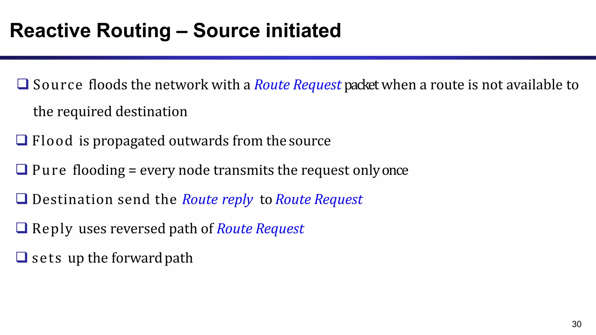
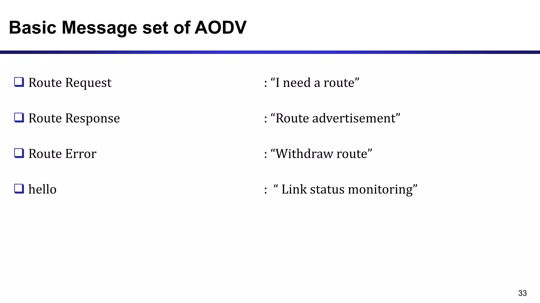
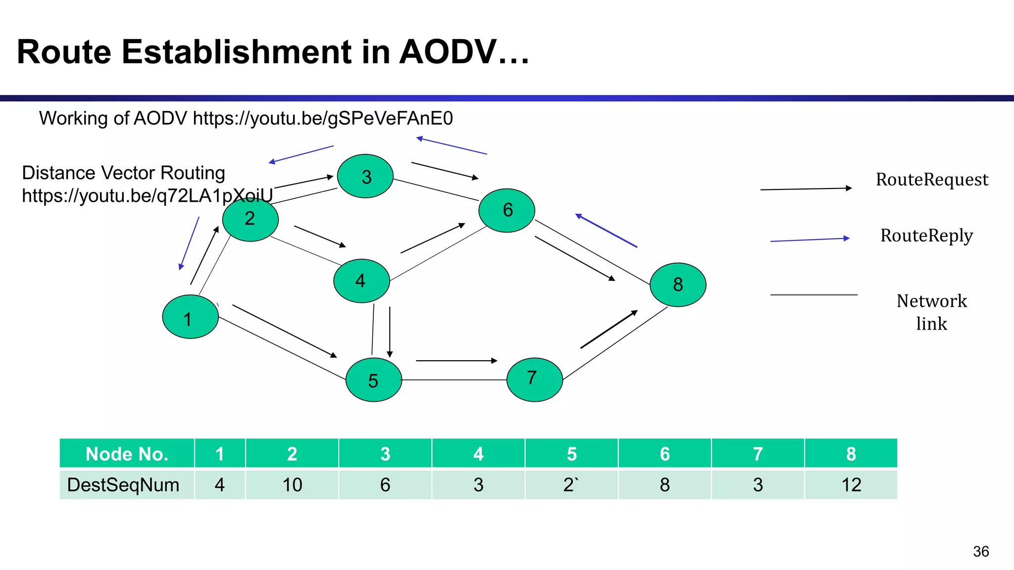
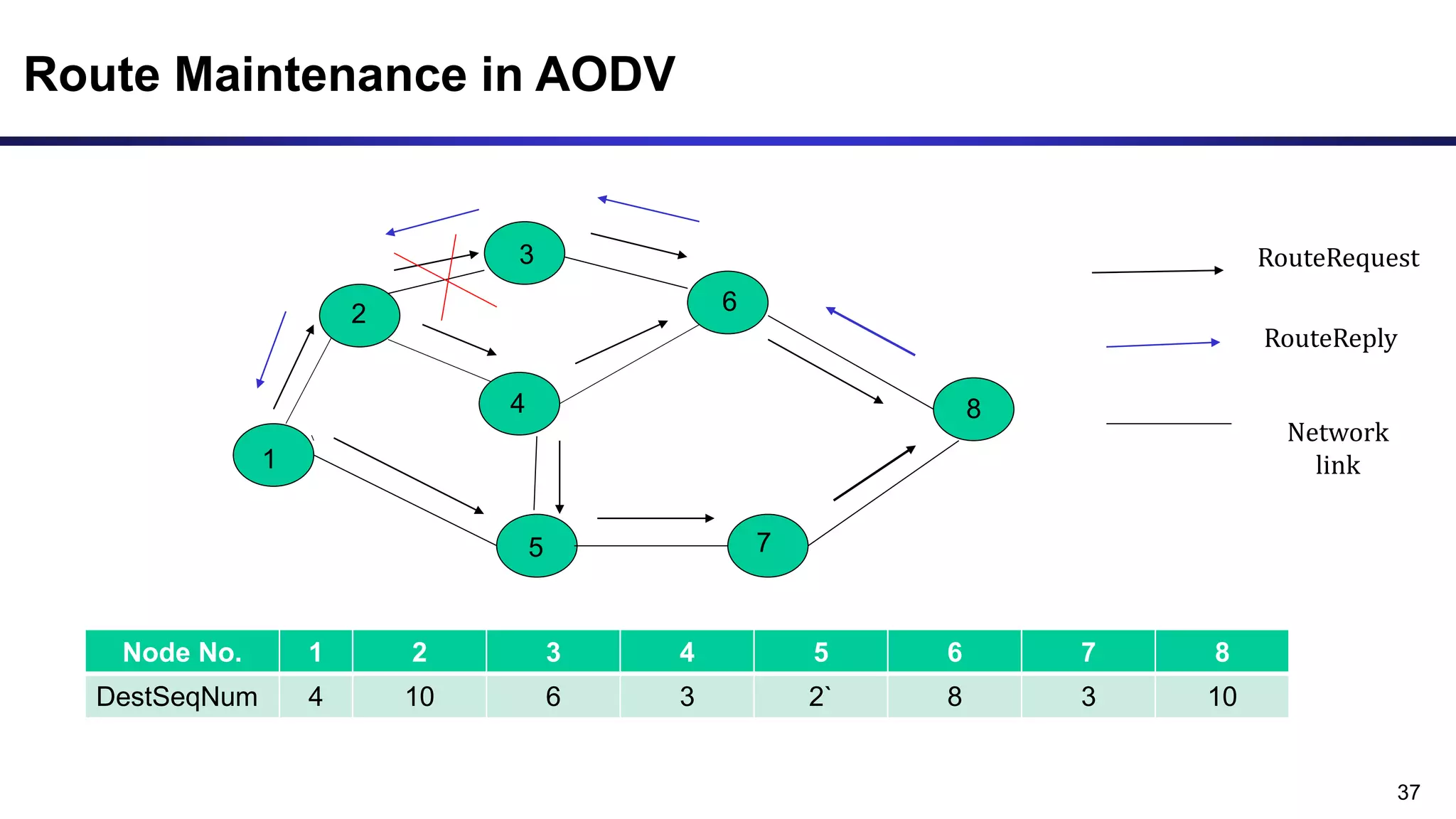
(SHREYA) Chakan Call Girls Just Call 7001035870 [ Cash on Delivery ] Pune Esc...
Ad hoc and wsn
1. AD HOC AND SENSOR NETWORKS
Presented by,
Dr. M.S.Gowtham, M.E., Ph.D.,
Associate Professor,
Department of Electronics and Communication Engineering
Karpagam Institute of Technology,
Coimbatore, Tamilnadu - 641105
2. Outline
Introduction
Features of Ad hoc Wireless networks
Issues in Ad hoc Wireless networks
Types of Ad hoc Wireless networks
Classifications of Routing Protocols
Table Driven Routing Protocols
Destination Sequenced Distance Vector (DSDV)
On–Demand Routing protocols
Ad hoc On–Demand Distance Vector Routing (AODV).
2
3. Introduction
Wireless Networking – refers to any
kind of networking that does not
involve cables
Wireless telecommunications networks
are implemented and administered
using a transmission system called
radio waves
Implementation takes place at the
physical level (layer) of the network
structure
It is a computer network that uses
wireless data connections
between network nodes
3
4. Network Topology
Infrastructure Based wireless network
numerous portable transceivers
communicate with each other and
with fixed transceivers and telephones
anywhere in the network, via base
stations
Ad hoc wireless network
Mesh networks :
fully connected network
Sensor networks :
Sensors are connected via wireless to
allow large scale collection of sensor
data.
4
5. Infrastructure based network
5
Network infrastructure is the hardware and software resources of an
entire network
that enable network connectivity, communication, operations and management of
an enterprise network. It provides the communication path and services between
users, processes, applications, services and external networks/the internet.
Connected to the wired LAN
The Wireless Access point used to extend the Coverage area of LAN network and to
connect wirelessly
Computers both in wired and wireless environment can connect with each other
6. Ad hoc wireless network
Ad hoc is a word that originally comes from Latin and means “for this” or "for this
situation.
Multi hop wireless network
The wireless hosts in ad hoc networks, communicate with each other without the
existing of a fixed infrastructure
Decentralized control
A mobile ad-hoc network can be connected to other fixed networks or to the Internet.
Most of the Ad-Hoc networks operates in ISM band
Peer to Peer communication
Additional feature described in IEEE 802.11 as independent basic service set (IBSS)
Packed switched network
6
8. Cellular network Vs Ad hoc wireless network
Cellular network
Communication through base station (BS)
Single-hop
Centralized management at BS
Long-term communication
Seamless connectivity
Homogeneous devices
Maintenance cost is high
Ad hoc wireless network
Peer-to-peer communication
Multi-hop, relay
Distributed management
Short-term, on-the-fly
Frequent breakup in link
Heterogeneous devices
Self Organizing , maintenance
properties are within the network
8
9. Benefits of wireless ad-hoc networks
Ad hoc networks do not require access points
Provide a low-cost way of direct client-to-client communication
Ad-hoc networks are easy to configure and offer an effective way to communicate
with devices nearby
Used efficiently under the condition when running cable is not feasible.
Ad-hoc networks are often secured to protect against attacks.
An ad-hoc network linking a small number of devices might be better than a regular
network with more users connected.
Self organizing
9
10. Disadvantages of ad hoc wireless networks
Devices in an ad-hoc network cannot disable Service Set Identifier(SSID)
broadcasting
Attackers can find and connect to an ad hoc device if they are within signal range
Wireless ad-hoc networks cannot bridge wired LANs or to the internet without
installing a special-purpose network gateway.
Devices can only use the internet if one of them is connected to and sharing it with
the others
Ad-hoc mode requires more system resources as the physical network layout
changes as devices are moved around
Limited wireless bandwidth
Frequent reconfiguration of network
10
11. Major Issues in Ad hoc wireless networks
Medium access scheme
Routing
Multicasting
Transport layer protocol
Pricing scheme
Quality of service provisioning
Self-organization
Security
Energy management
Addressing and service discovery
Scalability
Deployment considerations
11
12. Types of ad-hoc wireless networks
Mobile Ad hoc NEtwork (MANET)
involves mobile devices communicating directly with one another
a network of wireless mobile devices without an infrastructure
self-organizing and self-configuring
sometimes referred to as an "on-the-fly" or "spontaneous network.“
Internet-based Mobile Ad hoc NEtworks (iMANETs)
support internet protocols, such as TCP/IP and UDP
iMANET employs a network-layer routing protocol to connect mobile nodes
set up distributed routes automatically
12
13. Types of ad-hoc wireless networks…
Smartphone Ad hoc NEtworks (SPANs)
employ existing hardware, such as Wi-Fi and Bluetooth
software (protocols) used in smartphones to create peer-to-peer (P2P)
networks
does not rely on cellular carrier networks, wireless access points or traditional
network infrastructure.
support multihop communication
Vehicular Ad hoc Network (VANET)
communication between vehicles and roadside equipment
consists of groups of moving or stationary vehicles connected by a wireless
network
13
14. Issues in Designing Routing Protocol for Ad hoc network
Medium access scheme
Distributed operation
Synchronization
Hidden terminal
Access delay
Fairness
Resource reservation
Capability of power control
14
15. Desired Characteristics of routing protocol
Fault tolerant Distributed routing , thus reduced control over head
Adaptive to frequent topology changes
Route computation and maintenance must involve a minimum number of
Nodes and minimum connection setup time is desired.
It must be localized, as global state maintenance involves a huge state
propagation control overhead.
It must be loop-free and free from stale routes.
15
16. Desired Characteristics of routing protocol …
The number of packet collisions must be kept to a minimum by limiting
the number of broadcasts made by each node.
Quick convergence towards optimal route
optimal use of bandwidth, computing power, memory, and battery power.
Every node in the network should try to store stable local topology only
information regarding the
Good Quality of Service and to offer support for time-sensitive traffic.
16
17. Classification of routing protocols
Routing protocols for ad-hoc wireless networks can be classified based on:
routing information update mechanism:
Proactive, Reactive, Hybrid
usage of temporal information (e.g. cached routes):
Past temporal , Future temporal
usage of topology information:
Flat, Hierarchical
usage of specific resources :
Power-aware routing
Geographical information assisted routing
17
18. 18
Proactive protocols
Table Driven protocol
Traditional distributed shortest path protocols
Maintain routes between every host pair at all times
Based on periodic updates; High routing overhead
Example: DSDV (destination sequenced distance vector)
Reactive protocols
Determine route if and when needed
Source initiates route discovery
Network topology information is not maintained
Example: DSR (dynamic source routing)
Ad hoc On–demand Distance Vector Routing (AODV)
Routing Protocols
19. 19
Hybrid protocols
Adaptive
Combination of proactive and reactive
Example : ZRP (zone routing protocol)
Hierarchical protocols
choice of proactive and of reactive routing depends on the hierarchic level in
which a node resides
hierarchy could be based on geographical information or it could be based
on hop distance
Cluster Based Routing Protocol
Routing Protocols
20. Challenges of routing protocols in ad hoc networks
Movement of nodes:
Path breaks
Partitioning of a network
Inability to use protocols developed for fixed network
Bandwidth is a scarce resource:
Inability to have full information about topology
Control overhead must be minimized
Shared broadcast radio channel:
Nodes compete for sending packets
Collisions
Erroneous transmission medium:
Loss of routing packets
20
21. Destination Sequenced Distance Vector (DSDV) routing
protocol
Destination-Sequenced Distance Vector (DSDV) routing protocol is a pro-active, table-
driven routing protocol for MANETs
Developed by Charles E. Perkins and Pravin Bhagwat in 1994
Enhancement of the Bellman-Ford algorithm where each node maintains:
the shortest path to destination
the first node on this shortest path
It uses the hop count as metric in route selection
routes to all destinations are readily available at every node at all times
Routing Tables are also exchanged when significant changes in local topology are
observed by a node
No Loop in routing
Count to infinity problem is avoided
21
22. Route Advertisement in DSDV
Dest. Next Metric Seq Dest. Next Metric Seq Dest. Next Metric Seq.
A A 0 A-550 A A 1 A-550 A B
2
A-550
B B 1 B-100 B B 0 B-100 B B
1
B-100
C B 2 C-588 C C 1 C-588 C C
0
C-588
22
(A, 1, A-500)
(B, 0, B-102)
(C, 1, C-588)
(A, 1, A-500)
(B, 0, B-102)
(C, 1, C-588)
------------------------------------------------------------------------------------
Node A
Node B Broadcast
information
Node C
Node B
23. Route Advertisement in DSDV
Dest. Next Metric Seq Dest. Next Metric Seq Dest. Next Metric Seq.
A A 0 A-550 A A 1 A-550 A B
2
A-550
B B 1 B-102 B B 0 B-102 B B
1
B-102
C B 2 C-588 C C 1 C-588 C C
0
C-588
23
(A, 1, A-500)
(B, 0, B-102)
(C, 1, C-588)
(A, 1, A-500)
(B, 0, B-102)
(C, 1, C-588)
------------------------------------------------------------------------------------
Node A Node B Node C
24. Respond to Topology Changes in DSDV
Immediate advertisements
Information on new Routes, broken Links, metric change is immediately propagated
to neighbors
Full/Incremental Update:
Full Update: Send all routing information from own table
Incremental Update: Send only entries that has changed , make it fit into one single
packet
24
25. New Node addition using DSDV…
Dest. Next Hop Seq. Dest. Next Hop Seq. Dest. Next Hop Seq. Dest. Next Hop Seq.
A A 0 A-550 A A 1 A-550 A B 2 A-550 A C 3 A-550
B B 1 B-104 B B 0 B-104 B B 1 B-104 B C 2 B-104
C B 2 C-590 C C 1 C-592 C C 0 C-592 C C 1 C-592
D C 2 D-000 D D 1 D-000 D D 0 D-000
25
Node A Node B Node D
Node C
(A, 2, A-550)
(B, 1, B-102)
(C, 0, C-592)
(D, 1, D-000)
(A, 2, A-550)
(B, 1, B-102)
(C, 0, C-592)
(D, 1, D-000)
26. Link Break in ad hoc network
Dest. Next Hop Seq. Dest. Next Hop Seq. Dest. Next Hop Seq. Dest. Next Hop Seq.
A A 0 A-550 A A 1 A-550 A B 2 A-550 A C 3 A-550
B B 1 B-104 B B 0 B-104 B B 1 B-104 B C 2 B-104
C B 2 C-590 C C 1 C-592 C C 0 C-592 C C 1 C-592
D B 3 D-100 D C 2 D-100 D D ∞ D-101 D D 0 D-101
26
Node A Node B Node D
Node C
(A, 2,A-550)
(B, 1,B-102)
(C, 0,C-592)
(D ∞,D-101)
B does its broadcast thus no impact on C
C has higher sequence number for destination D
No loop , no count to infinity on link break
27. Immediate Advertisement in ad hoc network
Dest. Next Hop Seq. Dest. Next Hop Seq. Dest. Next Hop Seq. Dest. Next Hop Seq.
A A 0 A-550 A A 1 A-550 A B 2 A-550 A C 3 A-550
B B 1 B-104 B B 0 B-104 B B 1 B-104 B C 2 B-104
C B 2 C-590 C C 1 C-592 C C 0 C-592 C C 1 C-592
D D ∞ D-101 D C ∞ D-101 D D ∞ D-101 D D 0 D-101
27
Node A Node B Node D
Node C
Node C detects the link break with node D
Immediate propagation of information to node B, the from node B to node A
Disconnected node sequence number is changed to odd number
28. Fluctuations in DSDV
• Fluctuations occurs when every time node does its broadcast and lead to unnecessary route
advertisements inthenetwork
28
Node A
Node C
Node D
Node B
(D,C,12,D-102)
(D,D,0,D-102)
(D,B,10,D-102)
29. On demand routing protocol
The route is discovered only when it is required/needed.
Process of route discovery occurs by flooding the route request packets throughout the
mobile network.
Route Discovery:
This phase determines the most optimal path for the transmission of data packets
between the source and the destination mobile nodes
Route Maintenance:
This phase performs the maintenance work of the route as the topology in the
mobile ad-hoc network is dynamic in nature
29
30. Reactive Routing – Source initiated
Source floods the network with a Route Request packet when a route is not available to
the required destination
Flood is propagated outwards from thesource
Pure flooding = every node transmits the request onlyonce
Destination send the Route reply to Route Request
Reply uses reversed path of Route Request
sets up the forwardpath
30
31. Advantages & disadvantages of Reactive routing protocol
Advantages:
eliminate periodic updates
adaptive to network dynamics
Disadvantages:
high flood-search overhead with mobility,
distributed traffic
high route acquisition latency
31
32. Ad-Hoc On Demand Vector Routing protocol (AODV)
Reactive or On-demand routing protocol
In AODV, the source node and the intermediate nodes store the next-hop information
corresponding to each flow for data packet transmission
AODV supports multicasting and unicasting within a uniform framework
Each route has a lifetime after which the route expires if it is not used
AODV maintains only one route between a source-destination pair
Routing table size is minimized by only including next hop information, not the entire
route to a destination node.
Sequence numbers for both destination and source are used.
Managing the sequence number is the key to efficient routing and route maintenance
32
33. Basic Message set of AODV
Route Request : “I need a route”
Route Response : “Route advertisement”
Route Error : “Withdraw route”
hello : “ Link status monitoring”
33
34. Fields of Routing Table in AODV
Destination IP address
Destination Sequence Number
Valid Destination Sequence Number Flag
Other state and routing flags
Network Interface
Hop Count (needed to reach destination)
Next Hop
Lifetime (route expiration or deletion time)
34
35. Route Establishment in AODV
Uses a destination sequence number (DestSeqNum) to determine an up-to-date path
to the destination.
A node updates its path information only if the DestSeqNum of the current packet
received is greater than the last DestSeqNum stored at the node.
A RouteRequest consist of following fields:
source identifier (SrcID),
destination identifier(DestID),
source sequence number (SrcSeqNum)
destination sequence number (DestSeqNum)
broadcast identifier (BcastID),
time to live (TTL)
35
38. Advantages & Disadvantages of AODV
Advantages
routes are established on demand and destination sequence numbers are used to find
the latest route to the destination
The connection setup delay is less
Disadvantages
intermediate nodes can lead to inconsistent routes if the source sequence number is
very old
multiple RouteReply packets in response to a single RouteRequest packet can lead to
heavy control overhead.
periodic beaconing leads to unnecessary bandwidth consumption.
39. Reference
C. Siva Ram Murthy and B. S. Manoj, ―Ad Hoc Wireless Networks
Architectures and Protocols‖, Prentice Hall, PTR, 2004.
39
40. 1. Passive, omni-directional sensors:
– Measure a physical quantity without actually manipulating the environment by active probing
– No notion of “direction” involved in these measurements and may be self powered
Eg: thermometer, light sensors, vibration, microphones, humidity, mechanical stress or tension in
materials, chemical sensors sensitive, smoke detectors, air pressure, etc
2. Passive, narrow-beam sensors:
– Are passive
– Have a well-defined notion of direction of measurement.
– Eg: Camera
3. Active sensors:
– Actively probes the environment
– Eg: a sonar or radar sensor or some types of seismic sensors
• Actuators:
– Are as diverse as sensors
– Usually are controlled by sensors and in turn trigger some function or device
SENSORS & ACTUATORS
41. CHALLENGES FOR WSNs
• TYPE OF SERVICE: Provide meaningful information and actions about a
given task, hence new paradigms of using such a network are required.
• QUALITY OF SERVICE: Packet delivery ratio is an insufficient. Adapted
concepts like reliable detection of events or the approximation of quality is
important.
• FAULT TOLERANCE: Nodes should be damage and failure tolerant.
• LIFE TIME: WSN nodes rely on a limited supply of energy(batteries).
Replacing these energy sources in the field is not practical, hence life time of
WSN becomes important figure of merit.
42. • SCALIBILITY: Protocols used must be able to support large no. of nodes.
• WIDE RANGE OF DENSITIES:
Density of network: No. of nodes per unit area & it vary with applications
• PROGRAMMABILITY: Nodes should be programmable, and their
programming must be changeable during operation when new tasks become
important.
• MAINTAINABILITY: Environment of a WSN and the WSN itself change, the
system has to adapt. Has to maintain itself; able to interact with external
maintenance mechanisms.
CHALLENGES FOR WSNs
43. ENABLING TECHNOLOGIES FOR WSNs
1) Miniaturization of hardware
2) R e d u c e d c h i p s i z e & i m p r o ve d e ff i c ie n cy
accompanied by reduced cost
3) The actual sensing element
These 3 parts have to be accompanied by power supply.
A sensor node has a device energy scavenging.
44. WSN Application Examples
• DISASTER RELIEF APPLICATIONS: Wildfire, sensors
produce a “temperature map” of the area.
• ENVIRONMENT CONTROL AND BIODIVERSITY
MAPPING: Chemical pollutants, surveillance of the marine
ground floor and survey on no. of plant and animal species that
live in a particular habitat.
• INTELLIGENT BUILDINGS: monitoring of temperature,
airflow, humidity and other physical parameters in a building
- reduce energy consumption. Also Mechanical stress level
buildings.
45. • M A C H I N E S U R V E I L L A N C E & P R E V E N T I V E
MAINTANANCE: Sensor nodes are fixed at difficult-to- reach
areas of machinery to detect vibration patterns.
• FACILITY MANAGEMENT: Detection of intruders, tracking
vehicle’s position, scanning chemical leakage in chemical plants.
• PRECISION AGRICULTURE: Fertilizing by placing
humidity/soil composition sensors into fields. Also pest control,
livestock breeding can be improved.
N.Kumaratharan, Prof/ECE, SVCE
WSN Application Examples
46. • MEDICINE & HEALTH CARE: Long-term surveillance of
patients and automatic drug administration. Also used in patient-
doctor tracking system.
• LOGISTICS: Used for simple tracking of goods during
transportation or to facilitate inventory tracking in stores and
warehouses.
• TELEMATICS: Used to gather information about traffic
conditions at a higher resolution(intelligent roadside)
N.Kumaratharan, Prof/ECE, SVCE
WSN Application Examples
48. CONTROLLER
• Collects data from the sensors, processes the data, decides
when and where to send it, receives data from other sensor
nodes, and decides on the actuator’s behaviour.
• Executes various programs, ranging from time-critical signal
processing and communication protocols to application
programs.
• Microcontrollers, microprocessors, FPGAs, and ASICs can be
used as controllers
49. MEMORY
• Random Access Memory (RAM):
– Store intermediate sensor readings, packets from other nodes
– Comparatively faster
– Volatile in nature
• Read-only Memory (ROM) or Electrically Erasable Programmable Read-
only Memory (EEPROM):
– Store program code
• Flash Memory:
– Allows data to be erased or written in blocks instead of only a byte at a time
– Serve as intermediate storage of data in case RAM is insufficient or when the
power supply of RAM should be shut down for some time
– Longer delay and more consumption of energy
50. COMMUNICATION DEVICE
– Used to exchange data between individualnodes.
• Choice of transmission medium
– There are different mediums for wireless communication. Some are,
• Radio frequencies
• Optical communication
• Ultrasound
• Magnetic inductance
– RF-based Communication :
• Most suitable for WSN applications; since it provides
– Relatively long range and high data rates
– Acceptable error rates at reasonable energy expenditure and
– No line of sight between sender and receiver required
• Frequencies used: between about 433 MHz and 2.4 GHz
51. COMMUNICATION DEVICE
• TRANSCEIVERS:
– Device capable of doing both transmission and reception.
– But usually, only half duplex operation is realized.
–Transceiver tasks and characteristics
1.Service to upper layer:
• Offer certain services to the upper layers, most notably to the Medium Access
Control (MAC) layer.
• The service is mostly packet oriented.
2.Power consumption and energy efficiency:
• Energy efficiency is the energy required to transmit and receive a single bit.
• Transceivers should be switchable between different states (Eg. Idle, sleep and
active).
52. 3.Carrier frequency and multiple channels
• Transceivers are available for different carrier frequencies.
• Some provides several carrier frequencies (“channels”)
4.State change times and energy:
• Transceiver can operate in different modes: sending or receiving, use
different channels, or be in different power-safe states.
• Important figures of merit are the time and the energy required to change
between two states.
5.Data rates:
• The gross data rate is determined by carrier frequency and used
bandwidth together with modulation and coding.
COMMUNICATION DEVICE
53. 6.Modulations
• Transceivers can support one or several of on/off-keying (ASK,
FSK etc.)
7.Coding
8.Transmission power control 9.Noise
figure:
NF =SNRI/SNRo
NF dB = SNRI dB − SNRO dB
10.Gain:
• Ratio of the output signal power to the input signal power
• Expressed in dB
COMMUNICATION DEVICE
54. COMMUNICATION DEVICE
11. Power Efficiency
• Efficiency of radio front end: Ratio of the radiated power to the overall power
consumed by the front end.
• Efficiency of power amplifier: Ratio of the output signal’s power to the power
consumed by the overall power amplifier.
12. Receiver sensitivity (given in dBm):
• The minimum signal power at the receiver needed to achieve a prescribed Eb/N0 or a
prescribed bit/packet error rate.
13. Out of band emission:
• The inverse to adjacent channel suppression is the out of band emission of a
transmitter.
55. COMMUNICATION DEVICE
• It is considered in absence of interference
• It depends on:
– the transmission power
– the antenna characteristics
– the attenuation caused by the environment
– the used carrier frequency
– the modulation/coding scheme that is used
– the bit error rate that one is willing to accept at the receiver
– the quality of the receiver- sensitivity.
56. COMMUNICATION DEVICE (Contd..)
16. Blocking performance:
• Achieved bit error rate in the presence of an interferer.
17. Carrier sense and RSSI:
• To sense whether the wireless channel, the carrier, is busy (another node is
transmitting).
• RSSI (Received Signal Strength Indicator): The signal strength at which an
incoming data packet has been received.
18. Voltage range:
• Transceivers should operate reliably over a range of supply voltages.
57. • Transceiver structure:
• Radio frequency front end:
frequency band.
Analog signal processing in the actual radio
• Baseband processor: signal processing in the digital domain and communicates with a
sensor node’s processor or other digital circuitry
• RF front end:
– Power Amplifier (PA): accepts up-converted signals from the IF or baseband part and
amplifies them for transmission over the antenna.
– Low Noise Amplifier (LNA): amplifies incoming signals without significantly reducing
SNR. Always active and can consume a significant fraction of transceiver’s energy.
– Local oscillators or voltage-controlled oscillators and mixers: used for frequency
conversion from the RF spectrum to intermediate frequencies or to the
baseband.
Transceiver Design Considerations
59. • Mostly four states:
1.Transmit : The transmit part of the transceiver is active and the
antenna radiates energy.
2.Receive : The receive part is active
3.Idle: Transceiver is ready to receive but is not currently receiving
anything. In this state, many parts of the receive circuitry are active,
and others can be switched off.
4.Sleep : Significant parts of the transceiver are switched off. sleep
states differ in the amount of circuitry switched off and in the associated
recovery times and startup energy
Transceiver Operational States
60. 1.Wakeup radioC:OMMUNICATION DEVICE (Contd..)
– Wakeup receivers: receiver specialized to notify an incoming packet; upon such an event,
the main receiver can be turned on and perform the actual reception of the packet.
2. Spread-spectrum transceivers:
– High performance transceivers with reduced interference.
– Complex hardware and high cost.
3. Ultrawideband communication:
– Very large bandwidth is used to directly transmit digital sequence as very short impulses which occupy
few Hertz up to the range of several GHz
– Sender and receiver has to be synchronized.
– Overlapping with conventional radio system can occur
– Small transmitting power is needed.
– Very high data rate can be realized over a short distance
– can easily penetrate obstacles such as doors.
– UWB transmitters are simpler where as receivers are more complex
Advanced Radio Concepts
61. COMMUNICATION DEVICE (Contd..)
1. Optical
– Optical links can be used between sensor nodes for communication
– Very small energy per bit required for both generating and detecting optical light
– Communication can take place concurrently with only negligible interference.
– Communicating peers need to have a line of sight connection
– Strongly influenced by weather conditions
2. Ultrasound
– Used where Radio or optical waves can not penetrate the surrounding medium
– Travels relatively long distances at comparably low power.
– Used for surveillance of marine ground floor erosion
– Used as a secondary means of communication with a different propagation speed
Examples of radio transceivers RFM TR1000 family, Hardware accelerators (Mica motes), Chipcon
CC1000 and CC2420 family, Infineon TDA 525x family, Ember EM2420 RF transceiver,
Non Radio Frequency Wireless Communication
62. • Energy s avings and overheads for sleep mo
Energy Consumption of Sensor Nodes
Main consumers: controller, radio front ends, memory, and depending on type, the sensors.
• t1 : Time at which the decision whether or not a component is to be put into sleep mode
should be taken to reduce power consumption from Pactive to Psleep.
• tevent : Time at which next event occurs
• Total energy wasted by idling at active time: Eactive = Pactive(tevent −t1)
•τdown: Time taken by the node to reach sleep mode from active mode
63. • Microcontroller energy consumption
• Embedded controllers commonly implement the concept of multiple operational states
• Examples:
1. Intel Strong ARM
– Provides three sleepmodes:
1. Normal mode: All parts of the processor are fully powered. Power consumption
is up to400 mW.
2. Idle mode: Clocks to the CPU are stopped; clocks that pertain to peripherals are
active. Any interrupt will cause return to normal mode. Power consumption is
up to 100 mW.
3. Sleep mode: Only the real-time clock remains active. Wakeup occurs after a timer
interrupt and takes up to 160ms. Power consumption is up to 50 μW.
Energy Consumption of Sensor Nodes
64. Energy consumption of sensor nodes (Contd..)
2. Texas Instruments MSP 430
• Fully operational mode: consumes about 1.2 mW
• There are four sleep modes.
– LPM4 ,deepest sleep mode :Consumes 0.3 μW. Only the controller is woken up
by external interrupts.
– LPM3, next higher mode: A clock is used for scheduled wake ups.
Consumes about 6 μW.
3. Atmel ATmega
• The Atmel ATmega 128L has six different modes of power consumption.
• Power consumption varies between 6 mW and 15 mW in idle and active modes and
is about 75 μW in power-down modes.
Energy Consumption of Sensor Nodes
65. Energy consumption of sensor nodes (Contd..)
• Dynamic voltage scaling
• Another technique that is used for saving power is to use a continuous notion of
functionality/power adaptation by adapting the speed with which a controller operates
instead of using different operational states.
• The supply voltage can be reduced at lower clock rates still guaranteeing correct
operation.
Memory:
• On-chip memory of a microcontroller and FLASH memory consumes lesser energy;
hence more appropriate for WSNs.
Radio transceivers
• Has two important tasks: transmitting and receiving data between a pair of nodes.
• Can operate in different modes
Energy Consumption of Sensor Nodes
66. Basic scenarios: Wireless Sensor Networks
Sensor network scenarios
Sources: Any entity that provides data/measurements
Sinks:
Source
Sink
Si
nk
Applications: Usually, machine to machine, often limited
amounts of data
Inte
rnet
Source
Sink
Source
69. Different sources of mobility
WSN Node mobility
A node participating as source/sink (or destination) or a relay node might move around
Deliberately, self-propelled or by external force; targeted or at random
Happens in both WSN and MANET
WSN Sink mobility
71. Optimization goals and figures of merit
• Quality of service
• Event detection/reporting probability:
– The probability that an event that actually occurred is not detected/not reported to
an information sink that is interested in such an event
– Eg: Not reporting a fire alarm to a surveillance station
• Event classification error: Events are not only to be detected but also to be classified,
the error in classification must be small.
• Event detection delay: The delay between detecting an event and reporting it to any/all
interested sinks
• Missing reports: In applications that require periodic reporting, the probability of
undelivered reports should be small.
72. Optimization goals and figures of merit (Contd..)
• Approximation accuracy:
– The Tracking applications mustaverage/max absolute or relative error with respect to
the actual function that occurs in function approximation applications
– E.g. approximating the temperature as a function of location for a given area
• Tracking accuracy:
– not miss an object to be tracked.
– The reported position should be as close to the real position as possible, and the error
should be small.
• Energy efficiency
• Energy per correctly received bit: Average energy spent, counting all sources of energy
consumption at all possible intermediate hops, to transport one bit of information from the
source to the destination
Optimization goals and figures of merit
73. )
Scalability
Ability to maintain performance characteristics irrespective of the size of the network
Robustness
WSN should not fail just because a limited number of nodes run out of energy, or because
their environment changes and break up existing radio links between two nodes
These failures have to be compensated; for example, by finding other routes.
Optimization goals and figures of merit
74. Text Book & References
• Text Book
• Holger Karl , Andreas willig, ―Protocol and Architecture for Wireless Sensor Networks‖,
John wiley publication, Jan 2006.
• References
1. Feng Zhao, Leonidas Guibas, ―Wireless Sensor Networks: an information processing
approach‖, Elsevier publication, 2004.
2. Charles E. Perkins, ―Ad Hoc Networking‖, Addison Wesley, 2000.
3. I.F. Akyildiz, W. Su, Sankarasubramaniam, E. Cayirci, ―Wireless sensor networks: a survey‖,
computer networks, Elsevier, 2002, 394 - 422.