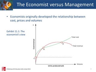
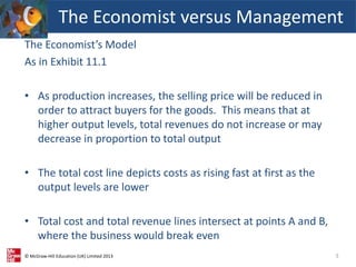
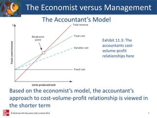
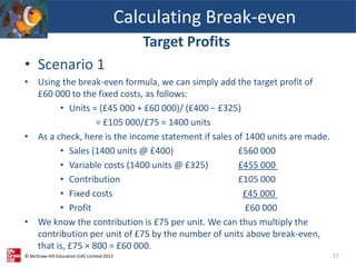
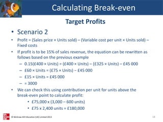
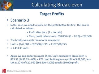
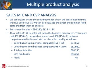
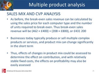
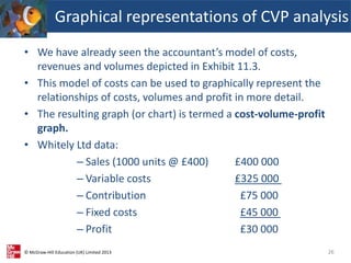
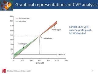
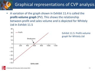
Chapter11.ppt/Cost Volume Profit Analysis

© McGraw-Hill Education (UK) Limited 2013
Short-Term
Decision Making:
Cost-Volume-
Profit Analysis
Chapter 11
1

• LO1 Calculate the level of sales or business activity
needed to break even or earn a desired profit
• LO2 Determine the revenue required to break even or
earn a desired profit
• LO3 Apply cost-volume-profit analysis in a multi-
product setting
• LO4 Graphically depict the relationship between costs,
volume and profits
• LO5 Consider impacts of uncertainty and change in
variables on cost-volume-profit analysis
Learning Outcomes
2

• Cost-volume-profit (CVP) analysis is a very useful tool for
managers, accountants and business owners in making short-
term decisions.
• CVP analysis brings together the costs and revenues of a
business and emphasises the relationship with volumes
• It helps to answer questions such as ‘How much do I need to
sell to cover my costs?’ or
• ‘How will an increase in costs affect the sales level required to
maintain current profit levels?’
Introduction
3

• Economists originally developed the relationship between
cost, prices and volumes
The Economist versus Management
4
Exhibit 11.1: The
economist’s view

The Economist’s Model
As in Exhibit 11.1
• As production increases, the selling price will be reduced in
order to attract buyers for the goods. This means that at
higher output levels, total revenues do not increase or may
decrease in proportion to total output
• The total cost line depicts costs as rising fast at first as the
output levels are lower
• Total cost and total revenue lines intersect at points A and B,
where the business would break even
5

The Economist’s Model of costs
6
Exhibit 11.2:
The
economist’s
variable cost
function

• Economists assume that variable costs per unit
initially declines – increasing returns to scale
• Between output levels V1 and V2, the organization is
operating at its most efficient level
• When output exceeds capacity, variable cost per unit
increases; this is called decreasing returns to scale
7

The Accountant’s Model
8
Based on the economist’s model, the accountant’s
approach to cost-volume-profit relationship is viewed in
the shorter term
Exhibit 11.3: The
accountants cost-
volume-profit
relationships here

The Accountant’s Model
• In the short term, output is likely to be relatively stable, or at
least within a stable range
• In this model total revenues and costs are assumed to follow a
linear pattern
• The fixed cost is constant, this is valid in the short term. Total
costs (fixed and variable) will rise as output increases
• The intersection between total costs line and total revenue
line is called the break-even point
9

• To use CVP analysis as a decision-making tool, the
following assumptions on cost are important, as
without them it would not be possible to calculate a
break-even point.
– Costs are assumed to remain relatively stable in
the short term
– Fixed costs are costs incurred regardless of output
– Variable costs increase as output increases
Calculating Break-even
10

• The point where costs are covered and no
profit is made is called the break-even point
• Separate costs into fixed and variable
• The profit of a business can be represented in
the following equation:
Profit = Sales revenue – Variable costs – Fixed costs
11

• The previous equation can be expanded by
expressing sales and variable costs
– Profit = (Sales Price*Units sold) –
(Variable cost per unit * Units sold) – Fixed costs
– Example Whitely Ltd
• Sales (1,000 units @ £400) £400 000
• Variable costs £325 000
• Contribution £75 000
• Fixed costs £45 000
• Profit £30 000
12

• 0 = (£400 × Units) – (£325 × Units) – £45 000
–Units = 45,000/75 = 600
• We can check this as follows:
• Sales (600 units @ £400) £240 000
• Variable costs (600 units @ £325) £195,000
• Profit £0
13

• We can calculate break-even in units using
contribution
• Contribution is sales revenue less variable costs
– Profit = (Units sold x Contribution per unit) – Fixed Costs
• Solving this equation we obtain the formula for
break-even:
Break-even in units = Fixed costs
Contribution per unit
Break-even in units = £45,000 = 600 units
(£400-325)
14

Target Profits
• The break-even point is useful information for
any business
• The techniques illustrated for break-even can
also be used to determine how many units
need to be sold to achieve a targeted profit
• We can use the break-even formula to
calculate the units required to achieve this
desired profit
15

Target Profits
• Using the Whitely Ltd example calculate the
units required to attain the following target
profit scenarios:
– Scenario 1: Obtain a profit of £60 000
– Scenario 2: Obtain a profit of 15 per cent of sales
revenue
– Scenario 3: Obtain a profit after tax of £50 000,
where the tax rate is 20 per cent.
16

Target Profits
• Scenario 1
• Using the break-even formula, we can simply add the target profit of
£60 000 to the fixed costs, as follows:
• Units = (£45 000 + £60 000)/ (£400 − £325)
= £105 000/£75 = 1400 units
• As a check, here is the income statement if sales of 1400 units are made.
• Sales (1400 units @ £400) £560 000
• Variable costs (1400 units @ £325) £455 000
• Profit £60 000
• We know the contribution is £75 per unit. We can thus multiply the
contribution per unit of £75 by the number of units above break-even,
that is, £75 × 800 = £60 000.
17

Target Profits
• Scenario 2
• Profit = (Sales price × Units sold) – (Variable cost per unit × Units sold) –
Fixed costs
• If profit is to be 15% of sales revenue, the equation can be rewritten as
follows based on the previous example
– 0.15(£400 × Units) = (£400 × Units) – (£325 × Units) – £45 000
– £60 × Units = (£75 × Units) − £45 000
– £15 × Units = £45 000
– = 3000
• We can check this using contribution per unit for units above the
break-even point to calculate profit:
• £75,000 x (3,000 – 600 units)
• £75 x 2,400 units = £180,000
18

Target Profits
• Scenario 3
• In this case, we need to work out the profit before tax first. This can be
calculated as follows:
» Profit after tax − (1 − tax rate)
» Thus, profit before tax is: £50,000 × (1 − 0.20) = £62,500
• The break-even units can now be calculated.
• Units = (£45,000 + £62,500)/(£75) = £107,500/£75
• = 1 433.33 units
• Again, we can perform a quick check. Units sold above break-even is
833.33 (1433.33 − 600) × £75 contribution gives a profit of £62,500, less
tax at 20 % of £12,500 (£62 500 × 20%) equals £50,000 profit.
19

Target Profits
• Contribution margin ratio
• This ratio is the contribution as a proportion of sales.
• In the example, the contribution margin ratio is 0.1875 (£75/£400).
• As CVP analysis assumes costs and prices are constant in the short term,
then the contribution margin ratio is also constant. Thus, it can be used in
the break-even formula used previously.
– Profit = Sales revenue – Variable costs – Fixed costs
– We can insert the contribution margin ratio as follows:
– Profit = (Sales Revenue × CM ratio) – Fixed costs
• At break-even, profit is nil so this equation can be solved as follows:
• Sales revenue = Fixed costs/ CM ratio
• Sales revenue = £ 45 000 = £240,000
0.1875
20

• Thus far, the examples given have presented a single product
scenario.
• In reality, most businesses will make and sell many products. CVP
analysis can be used in multiple product scenarios
• Assume Whitely Ltd manufactures personal and business
computers
Multiple product analysis
21
Personal
computer
Business
computer
Total
Sales price £ 400 800
Units 1200 800
£ £ £
Sales 480 000 640,000 1,120 000
Variable costs 390 000 480,000 870,000
Contribution 90,000 160,000 250,000
Direct fixed costs 30,000 40,000 70,000
Profit per product 60,000 120,000 180,000
Common fixed
costs
26,250
Operating profit 153,750

22
• There are two types of fixed costs in the example above.
– Direct fixed costs are costs which can be traced to the product and
would not be incurred if the product was not made.
– Common fixed costs are those which are not traceable to either
product, and would remain if either were discontinued
• It is possible to calculate a break-even point for each computer type
separately. The contribution per unit for the personal computer is
(£90,000/1200 units) £75 and (£160,000/800 units) and £200 for the
business computer. The break-even point in sales units is thus:
– Personal computer £30,000 £75 units = 400
– Business computer £40,000 £200 units = 200

SALES MIX AND CVP ANALYSIS
• Sales mix refers to the relative proportions of products sold. It
can be measured in terms of units or sales revenue
• A sales mix in units will typically not be the same as a sales
mix in revenue as the prices of products are unlikely to be
identical
• To begin, we need to calculate the contribution for each sales
mix bundle as follows
23
Product Unit Contribution Mix Bundle Contribution
Personal computer £75 3 £225 (3 x £75)
Business computer £200 2 £400 (2 x £200)

• We can equate this to the contribution per unit in the break-even formula
we have used thus far. We can also now add the direct and common fixed
costs and treat them as one cost
• Break-even bundles = £96,250/ £625 = 154
• Thus, sales of 154 bundles will mean the business breaks even. This means
that 462 (154 × 3) personal computers and 308 (154 × 2) business
computers need to be sold. We can check this quickly as follows:
– Contribution from personal computer (462 × £75) £34 650
– Contribution from business computer (308 × £200) £61 600
– Total contribution £96 250
– Less fixed costs £96 250
– Profit Nil
24

• As before, the break-even sales revenue can be calculated by
using the sales price for each computer type and the number
of units required to break even. Thus break-even sales
revenue will be (462 × £400) + (208 × £800), or £431 200
• Businesses today typically produce or sell multiple complex
products or services, and product mix can change significantly
in the short term
• Thus, effects of changes in product mix could be assessed to
determine the effect on contribution, and with relatively
stable fixed costs, the effects on profitability may also be
easily assessed
25

• We have already seen the accountant’s model of costs,
revenues and volumes depicted in Exhibit 11.3.
• This model of costs can be used to graphically represent the
relationships of costs, volumes and profit in more detail.
• The resulting graph (or chart) is termed a cost-volume-profit
graph.
• Whitely Ltd data:
– Sales (1000 units @ £400) £400 000
– Variable costs £325 000
– Contribution £75 000
– Fixed costs £45 000
– Profit £30 000
Graphical representations of CVP analysis
26

27
Exhibit 11.4: Cost-
volume-profit graph
for Whitely Ltd

• A variation of the graph shown in Exhibit 11.4 is called the
profit-volume graph (PV). This shows the relationship
between profit and sales volume and is depicted for Whitely
Ltd in Exhibit 11.5
28
Exhibit 11.5: Profit-volume
graph for Whitely Ltd

• The profit-volume graph for Whitely Ltd is drawn by again choosing some
known points. For example, we know that at zero output a loss equal to
the fixed costs (£45,000) occurs. At break-even point the profit is zero, and
as given, when output is 1000 units profit is £30,000.
• A profit-volume graph can be used to access the profit or loss at any level
of output, but it does not reflect the nature of costs, that is, fixed versus
variable.
• In multi-product scenarios, a profit-volume type chart is used to depict the
profit and sales of each product. The chart typically starts with the product
with the highest contribution to sales ratio and plots the cumulative sales
and profit by adding each additional product.
• The point at which profit is zero is the highest sales level at which
break-even occurs. An example is given in the exercises at the end of the
chapter
29

• You might question why use a graphical method
when the calculations can be done easily, as shown
earlier in the chapter.
• Remember that one of the key roles of a
management accountant is to provide information to
managers for decision making.
• Information in a graphical format is quite common,
and readily understood and accepted by managers.
30

• The accountant’s model on cost-volume- profit
makes a number of assumptions, the main ones
being:
1) Costs and revenues are linear functions of
output.
2) It is assumed that costs and prices remain
constant within a relevant range.
3) All units produced are sold.
4) In multiple product scenarios, sales mix is
known and remains constant.
5) All prices and costs are known with certainty
Assumptions of CVP
31

• The first assumption can be seen in Exhibit 11.4. That is, as output
increases, costs and sales increase in proportion. This is depicted by
straight, evenly sloped lines for costs and revenues.
• In practice, this may not be so, as cost and revenues may increase or
decrease as output varies. This takes us back to the economist’s model
depicted earlier. However, it is likely that costs and revenues do behave in
a linear fashion in the short term and within a relevant range, suggesting
the first two assumptions are reasonably valid.
• The third assumption is likely to be unrealistic, as some inventory is always
possible. However, in the context of the decisions to be made using CVP
analysis, we are looking to cover all costs of a particular period of time.
• The fourth assumption is also likely to be unrealistic as sales mix will vary.
• Finally, while most businesses have a good knowledge of costs, it is
unlikely that any business can be absolutely certain that its costs, and
classification of costs, are correct.
Assumptions of CVP
32

Margin of Safety
• As noted above, an important assumption of CVP
analysis is that costs and revenues are known with
certainty.
• This is unlikely to be the case in reality, but if
managers and accountants have a good knowledge
of underlying costs they can use this knowledge to
(1) extend the concept of break-even to a band or
range, (2) assess how risky the business or product
cost structure is and, (3) conduct ‘what if’ or
sensitivity analysis.
Risk & Uncertainty
33

Margin of Safety
• The margin of safety is the number of units which
are expected to be sold above break-even.
• In equation format the Margin of safety
= Expected sales – Break-even sales
• The sales figure can be expressed in units or
monetary terms
• The margin of safety can be used by managers as a
rule-of-thumb to ensure sales are not lost to the
degree that the business fails to breakeven
Risk & Uncertainty
34

Operating leverage
Risk & Uncertainty
35
Operating leverage refers to relative amount of costs
that are fixed and variable in the cost structure of a
business
Exhibit 11.7: Cost-
volume-profit chart of
Whitely Ltd, including
margin of safety

Operating leverage
• The degree of operating leverage can be measured by taking
the contribution in proportion to profit as follows (remember
that contribution is sale minus variable costs):
• Degree of operating leverage = Contribution/Profit
• Assume a software company has invested £10 million into
developing and marketing an application, which sells for £45
per copy. Each copy costs the company £5 to sell. Sales
volume is expected to reach 1 million copies. The degree of
operating leverage can be calculated as follows:
» 1,000,000 x (£45- 5)
» 1,000,000 x (£45- 5) - £10,000,000
» = £40,000,000 / £30,000,000
Risk & Uncertainty
36

Operating leverage
• Thus, the degree of operating leverage is 1.33. This means that, for
example, a 25 per cent increase in sales volume would produce a 33 per
cent (25% × 1.33) increase in profits – here are the figures to prove this:
£million
Sales (1.25 m × £45) 56.25
Variable costs (1.25 × £5) 6.25
50.00
Fixed costs 10.00
Profit 40.00
• It’s important to have an appreciation of the degree of operating leverage
to assist managers in judging the effects of changes, the relative
proportion of fixed and variable costs
Risk & Uncertainty
37

• Sensitivity analysis is used in many aspects of business and
management accounting.
• It is in effect a ‘what if’ technique that examines effects of
changes in underlying assumptions of a business scenario
Sensitivity Analysis
38

• Any number of possible analyses could be quickly prepared in
a spreadsheet, but remember that spreadsheets are only as
useful as the data input to them
Sensitivity Analysis
39

• Management accountants assume costs and
revenues follow a linear pattern
• Using these assumptions, cost-volume-profit
analysis can determine breakeven, target
profits and effects of changes in cost structure
on profit
• Risk and uncertainty can be incorporated
using margin of safety and/or sensitivity
analysis
Summary
40

Chapter11.ppt/Cost Volume Profit Analysis

More Related Content

Similar to Chapter11.ppt/Cost Volume Profit Analysis

More from SrikantKapoor1

Recently uploaded

Chapter11.ppt/Cost Volume Profit Analysis