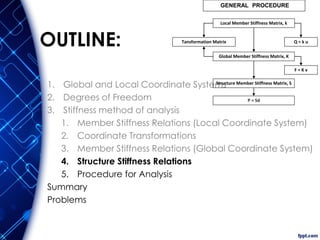
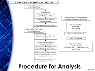
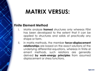
The document discusses the principles and methodologies of matrix structural analysis, emphasizing its importance for structural engineers in understanding performance under loads. It outlines various methods including classical, matrix, and finite element methods, while detailing the flexibility and stiffness methods, framed structures classification, and analytical modeling. Furthermore, it provides insight into matrix algebra, including types and operations, alongside the degrees of freedom and the stiffness method of analysis in the context of global and local coordinate systems.


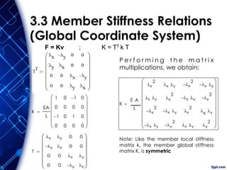
![3.3 Member Stiffness Relations
(Global Coordinate System)
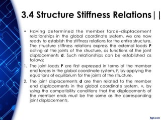
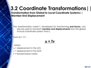
First, we substitute the local stiffness relations Q = ku into
the force transformation relations F = TTQ to obtain
F = TT (ku)
Then, by substituting the displacement transformation
relations, u = Tv into it, we determine that the desired
relationship between the member end forces F and end
displacements v, in the global coordinate system, is
F = TT [k(Tv)]
F = Kv Where:
K = TT k T
K = global member stiffness matrix](https://image.slidesharecdn.com/494999246-matrix-structural-analysis-truss-240619192534-335915de/85/494999246-Matrix-structural-analysis-Truss-pdf-77-320.jpg)