
Recommended
Recommended
More Related Content
Recently uploaded
Recently uploaded (20)
Featured
Featured (20)
3D‐dynamic modelling of Cretaceous sandstones at the outcrop scale (Galve Sub‐basin, Iberian Basin). Application to the studies of CO2 injection.
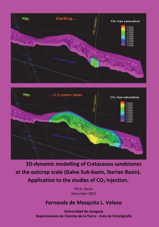
- 3. Cover Picture: CO2 gas saturation in the study case TsunV2 (constant rate regime) at the beginning of the injection simulation and three years later. https://es.linkedin.com/pub/fernanda‐de‐mesquita‐lobo‐veloso/9b/727/5a4 To access my LinkedIn profile:
- 4. This thesis is dedicated to my parents and my grandmother. Essa tese é dedicada aos meus pais e a minha avó. Esa tesis es dedicada a mis padres y mi abuela. “Agir, eis a inteligência verdadeira. Serei o que quiser. Mas tenho que querer o que for. O êxito está em ter êxito, e não em ter condições de êxito. Condições de palácio tem qualquer terra larga, mas onde estará o palácio se o não ficarem ali.” Fernando Pessoa (1888‐1935) Livro do desassossego (1982)
- 6. ACKNOWLEDGEMENTS This Ph.D. project was constructed and achieved with the assistance and advice of wonderful and competent persons, as well as with the support of University of Zaragoza, Ciencias de la Tierra department, laboratories as such the “Servicio de Preparación de Rocas y Materiales Duros” and members of Stratigraphy section. I offer my sincerest gratitude to my supervisors, Ana Rosa and Nieves Melendez who believed in this project and made me turn it in a Ph.D. They set excellent examples as successful and accomplished geologist scientist women (and mothers). I also thank Peter Frykman (from GEUS) who has supported me when it was still a project, then throughout its 4‐years’ development, and until now. I would like to thank the CNPq (Conselho Nacional de Pesquisa for the fellowship that I was awarded to conduct this Ph.D., and the Spain government (proyectos I+D, CGL2011‐23717) for the financial support to realize this research. Many thanks to Carlos Liesa, Antonio Casas and Luis Arlegui from the Geotransfer Research Group, and Enrique Arranz from petrography section, for their technical support to collect, prepare and analyze samples. Special thanks to Lope, Rocio and Roy of the stratigraphy section for the nice moments together (when I was there...). The international collaborations contributed immensely to my personal and professional competences. Thanks to Laboratoire de Fluides Complexes et ses Réservoirs of the UPPA (Université de Pau et de Pays de l’Adour), specially to Patrice Creux, Charles Aubourg and Jean Paul Caillot for the outstanding scientific stay and enlightening professional discussions. Thanks to GEUS (Geological Survey of Denmark), in particular to Carsten, Lars, Neils and everyone from the Reservoir department, for the short but intense and efficient stay during the final steps of the Ph.D. Also I would like to thank Schlumberger for making the modelling and simulation steps of this thesis possible using one of the best available commercial software (Petrel and Eclipse). I acknowledge the IEAGHG for the opportunity to join the 6th international interdisciplinary CCS (CO2 Capture and Storage) summer school
- 7. which permitted me to create and expand my network in the CCS, as well as to understand the CCS chain and deployment. I take this opportunity to express my gratitude to my climber friends (from Sagunto, Benidorm, Zaragoza and France) who helped me maintain a clear brain. Above all, I also thank my parents for the unceasing encouragement, support and attention. I am also grateful to Jean (my husband), who endured me through this venture and stayed on my side in all happy and painful moments. Thanks also to Françoise and Fabio for their understanding when reading my “English” version. Obrigada! Gracias! Merci! Thanks! Tak!
- 8. CONTENTS ABSTRACT ........................................................................................................................... 3 RESUMEN ............................................................................................................................ 5 RESUMO .............................................................................................................................. 7 1. INTRODUCTION ........................................................................................................ 11 1.1. THE STUDY AREA AND THE SELECTED OUTCROP: THE ALIAGA OUTCROP .................................... 13 1.2. GOALS ........................................................................................................................ 14 1.2.1. Framework .......................................................................................................... 14 1.3. STATE OF THE ART ......................................................................................................... 16 1.3.1. CO2 geological storage ........................................................................................ 16 1.3.2. Reservoir and outcrop heterogeneities ............................................................... 19 1.3.3. The numerical simulator: Eclipse300 .................................................................. 20 2. ALIAGA OUTCROP: SEDIMENTOLOGY AND PETROPHYSICS ........................................ 23 2.1. GEOLOGY AT THE BASIN SCALE ......................................................................................... 23 2.2. GEOLOGY AT THE OUTCROP SCALE .................................................................................... 29 2.2.1. Materials and methods ....................................................................................... 34 2.2.2. Sandstone deposits at the macroscale ................................................................ 37 2.2.2.1. Tsunami deposit .......................................................................................... 37 2.2.2.2. Barrier island ‐ tidal inlet deposit ................................................................ 39 2.2.3. Sandstone deposits at the microscale ................................................................. 43 2.2.3.1. Microfacies of the tsunami deposit ............................................................ 43 2.2.3.2. Microfacies of the barrier island ‐ tidal inlet deposit .................................. 50 2.3. PETROPHYSICS ............................................................................................................. 55 2.3.1. Petrophysics of the tsunami deposit ................................................................... 55 2.3.2. Petrophysics of the barrier island ‐ tidal inlet samples ....................................... 59 2.4. DISCUSSION ................................................................................................................. 63 2.5. CONCLUSION ............................................................................................................... 70 3. GEOLOGICAL AND PETROPHYSICAL MODELLING OF THE ALIAGA OUTCROP ............... 75 3.1. MATERIALS AND METHODS ............................................................................................. 76 3.1.1. Geostatistical analyses ........................................................................................ 76 3.1.1.1. Spatial data description .............................................................................. 77 3.1.1.2. Stochastic simulation algorithms ................................................................ 79 3.2. GRID CONSTRUCTION .................................................................................................... 81 3.2.1. Input surface/horizon construction ..................................................................... 83 3.2.2. Layering .............................................................................................................. 86 3.3. FACIES MODELLING ....................................................................................................... 87 3.3.1. Facies modeling of the tsunami deposit ............................................................. 87 3.3.1.1. Results of facies modelling of the tsunami deposit .................................... 92 3.3.2. Facies modelling of the barrier island‐tidal inlet deposit .................................... 96
- 9. 2 3.3.2.1. Results of facies modelling of the barrier island‐tidal inlet deposit ............ 99 3.3.3. Discussion on facies modelling .......................................................................... 103 3.3.3.1. Discussion on tsunami facies modelling .................................................... 104 3.3.3.2. Discussion on barrier island – tidal inlet deposit ...................................... 110 3.4. PETROPHYSICAL MODELLING ........................................................................................ 114 3.4.1. Petrophysical modelling of the tsunami deposit ............................................... 114 3.4.1.1. Porosity modelling of the tsunami deposit ............................................... 114 3.4.1.1.1. Results of porosity modelling of the tsunami deposit ...................... 117 3.4.1.2. Permeability modelling of the tsunami deposit ........................................ 121 3.4.1.2.1. Results of permeability modelling of the tsunami deposit ............... 122 3.4.2. Petrophysical modelling of the barrier island – tidal inlet deposit .................... 123 3.4.2.1. Porosity modelling of the barrier island – tidal inlet deposit .................... 123 3.4.2.1.1. Results of porosity modelling ........................................................... 126 3.4.2.2. Permeability modelling of the barrier island – tidal inlet deposit ............. 131 3.4.2.2.1. Results of permeability modelling .................................................... 131 3.4.3. Discussion on Petrophysical Modelling ............................................................. 134 3.5. MODELLING CONCLUSION ............................................................................................ 136 4. CO2 INJECTION IN THE TSUNAMI AND BARRIER ISLAND – TIDAL INLET RESERVOIRS AT THE OUTCROP SCALE ........................................................................................................141 4.1. RESERVOIR MODEL ..................................................................................................... 141 4.2. FLUID MODEL ............................................................................................................ 142 4.3. FLUID PROPERTIES ....................................................................................................... 145 4.3.1. Density .............................................................................................................. 145 4.3.2. Viscosity ............................................................................................................ 146 4.3.3. pH calculation ................................................................................................... 146 4.3.4. Saturation functions .......................................................................................... 146 4.3.5. Diffusion ............................................................................................................ 147 4.4. RESULTS OF RESERVOIR SIMULATION ............................................................................... 148 4.4.1. Simulation on the Tsunami reservoir ................................................................ 148 4.4.2. Simulation on the barrier island – tidal inlet deposit reservoir ......................... 152 4.4.3. Flow at the boundary grid blocks of reservoirs ................................................. 157 4.5. DISCUSSION ............................................................................................................... 158 4.6. CONCLUSION ............................................................................................................. 162 5. CONCLUSIONS AND PERSPECTIVE ............................................................................165 CONCLUSIONES Y PERSPECTIVA ........................................................................................173 REFERENCES .....................................................................................................................183
- 10. 3 ABSTRACT Geological and reservoir modelling are mandatory in studies that regard the geological storage of CO2. The aim of this study was to investigate the intra‐unit heterogeneity of the two sandstone deposits observed in the Aliaga outcrop at metre scales, and to examine how heterogeneity can impact the behaviour of CO2 in the zone close to the injector well during injection and post‐injection processes in a deep saline aquifer scenario. The Aliaga outcrop, is an 8400‐m² 2D vertical face in the upper part of the Camarillas Fm. (Early Cretaceous, Galve sub‐basin). The studied sandstone deposits correspond to a tsunami and a barrier island – tidal inlet, which were described in macroscale (centimetre to metric) and microscale (micron); further cores were drilled along outcrop to collect samples for porosity and permeability measurements. The two sandstone deposits were generated by distinct sedimentary processes under the same sedimentary system, and showed distinct petrophysical characteristics. The modelling process was different for each deposit, and honoured the petrophysical characteristics that were used to build the reservoir model post‐hoc. The petrophysics models reflected the sandy variability, which was represented by the facies distribution. The facies were defined as a function of the sand sorting at the petrographic scale. The tsunami facies and porosity distributions are homogeneous, whereas the barrier island‐tidal inlet facies and porosity distributions are heterogeneous. Porosity and permeability are strongly correlated in both deposits; thus, the permeability modelling was carried out as a function of the porosity model by applying a regression equation. Although the permeability is usually low (tens of mD), the two deposits behaved as a reservoir. At a short‐time scale (7 years), both reservoirs stored at least of 60% injected CO2, with the 20‐40% dissolved in the brine. At the sub‐metric scale, under the same reservoir conditions and fluid model parameters, the thickness of reservoir has the major impact in the amount of CO2 dissolution rather than the permeability contrast.
- 11. 4
- 12. 5 RESUMEN La modelización geológica y de reservorios es obligatoria en los estudios sobre el almacenamiento geológico de CO2. El objetivo de este estudio ha sido investigar las heterogeneidades intra‐capa en dos cuerpos arenosos a escala de afloramiento (escala métrica) observados en el afloramiento de Aliaga, y examinar cómo estas heterogeneidades pueden afectar al comportamiento del CO2 en la zona próxima al pozo inyector, durante los procesos de inyección y post‐inyección, en un escenario correspondiente a un acuífero salino profundo. El afloramiento de Aliaga, situado en la parte superior de la Fm. Camarillas (Cretácico Inferior, Subcuenca de Galve), tiene una superficie de afloramiento 2D de 8.400 m². Los dos cuerpos arenosos estudiados corresponden al depósito de un episodio de tsunami y de un complejo isla de barrera/inlet. Estos depósitos fueron cartografiados a escala de afloramiento y descritos a todas las escalas (desde la macroescala a la microescala) y además, en ellos, se extrajeron núcleos de sondeos sobre los que se realizaron las medidas de porosidad y permeabilidad. Ambos depósitos se generaron por procesos sedimentarios distintos dentro de un mismo sistema sedimentario (ambientes de back barrier) y muestran características petrofísicas distintas. El proceso de modelización fue diferente para cada depósito, y respetó las características petrofísicas que se emplearon para construir posteriormente el modelo de yacimiento. Los modelos petrofísicos reflejan principalmente la variabilidad de las areniscas, representada por la distribución de las distintas facies arenosas definidas. Estas facies arenosas han sido definidas a partir de la selección de las areniscas a escala petrográfica. La distribución de las facies del depósito de tsunami es homogénea, así como la distribución de su porosidad, mientras que en el depósito de isla de barrera/inlet, tanto la distribución de las facies como la de la porosidad son heterogéneas. La porosidad y permeabilidad están fuertemente correlacionados en ambos depósitos; por lo tanto, el modelo de permeabilidad se llevó a cabo como una función del modelo de porosidad mediante la aplicación de una ecuación de regresión.
- 13. 6 A pesar de que la permeabilidad es generalmente baja en ambos depósitos (decenas de mD), ambos se comportaron como reservorios. A una escala de tiempo corto (7 años), ambos reservorios almacenan al menos un 60% de todo el CO2 inyectado, con un 20‐40% de él disuelto en la salmuera. A escala submétrica, para las mismas condiciones de yacimiento y los mismos parámetros del modelo de fluido, la potencia del reservorio tiene un mayor impacto en la cantidad de disolución del CO2 que el contrate de permeabilidad del yacimiento.
- 14. 7 RESUMO A modelagem geológica torna‐se necessária em estudos para caracterização de um reservatório para armazenamento geológico de CO2. Com este propósito, o presente estudo teve como objetivo investigar as heterogeneidades intra‐layer (intracamadas) em dois corpos aflorantes de rochas areníticas, em escala métrica, do afloramento denominado Aliaga e analisar como essas heterogeneidades podem afetar o comportamento do CO2 na área próxima ao poço de injeção durante os processos de injeção e pós‐ injeção em um cenário de armazenamento em aqüífero salino profundo. O afloramento de Aliaga situa‐se na parte superior da Formação Camarillas, pertencente à sub‐bacia de Galve, considerada de idade do Cretáceo Inferior. Em superfície aflora abrangendo uma área de 8.400 m² (afloramento em 2D). Os dois corpos de arenito estudados para serem utilizados com reservatórios geológicos de CO2 correspondem a um episódio sedimentar relacionado a eventos proporcionados por tsunami e ilha barreira / canal inlet. Ambas as unidades foram gerados por diferentes processos deposicionais dentro do mesmo sistema sedimentar (parte continental da ilha barriera) e mostram diferentes características petrofísicas. Estas duas unidades foram mapeadas na escala de afloramento e descritas em escalas microscópica a macroscópica e, ainda, foram efetuadas sondagens e os testemunhos foram utilizados para obtenção das medições de porosidade e permeabilidade. O processo de modelagem aplicado foi distinto para cada unidade estudada, e assim, respeitadas suas características petrofísicas que foram utilizadas posteriormente para construir os modelos geológico dos reservatórios. Modelos petrofisicos refletem, principalmente, a variabilidade dos arenitos, representada pela distribuição dos vários fácies arenosos definidos. Estes fácies arenosos foram classificados a partir da seleção de grãos descritos em escala petrográfica. Os fácies do depósito de tsunami apresentam uma distribuição homogênea, assim como a porosidade, enquanto que os facies do depósito de ilha barreira/ canal inlet tanto a distribuição de fácies e a porosidade são heterogêneos. Porosidade e permeabilidade estão fortemente correlacionados em ambos os depósitos, por conseguinte, o modelo de
- 15. 8 permeabilidade foi realizado como uma função do modelo de porosidade por meio de uma equação de regressão . Embora a permeabilidade seja geralmente baixa em ambas as unidades (dezenas de mD), as mesmas podem se comportar como reservatórios. Numa escala de tempo curto, de aproximadamente 7 anos, ambos os reservatórios apresentam capacidade de armazenamento de, pelo menos, 60 % do CO2 injectado e entre 20 e 40 % desse CO2 de se dissolver na solução salina. Na escala submétrica, para as mesmas condições de reservatório e os mesmos parâmetros do modelo de fluido, a espessura do reservatório tem um impacto maior sobre a quantidade de CO2 dissolvido do que o contraste de permeabilidade do reservatório.
- 16. 9 CHAPTER 1 INTRODUCTION 1.1 The study area and the selected outcrop: The Aliaga outcrop_________________________________________13 1.2 Goals______________________________________14 1.3 State of the art______________________________16
- 17. 10
- 18. 11 1. Introduction The ‘greenhouse effect’ refers to processes that trap heat in the atmosphere and thus prevent heat loss to space. The effect is primarily the result of enhanced concentrations of carbon dioxide (CO2) and other gases in the atmosphere, that absorb and re‐radiate energy. Human activity related to the burning of fossil fuels is largely responsible for recent changes in the natural CO2 balance of the Earth–atmosphere system, and is thus responsible for the recent intensification of the greenhouse effect on Earth (IEAGHG, 2013). In Europe alone, the total emission of CO2 from the 28 member states (EU28) caused by human activity (excluding land use activities, land‐use changes and forestry; LULUCF) was 2.99 billion tonnes in 2012. The main source of CO2 emissions was public electricity and heat production (PEHP), which correspond to 27% of the total CO2 emission. Spain was responsible for 7.5% of the European CO2 emission, occupying 7th place in terms of emissions after Poland (EEA, 2015). In 2013, Spain produced only 28% of its PEHP, showing a strong dependency on imported energy (SEE, 2013), despite estimated carbon reserves in Spain which, in 1992, were ~3463.4 Mt (IGME, 2012); however, Spain’s carbon energy production in 2012 was only 21 Mt (IGME, 2012), or 1% of its estimated carbon reserves. Carbon dioxide capture and geological storage (CCS) is a bridging technology that will contribute to the mitigation of climate change, as it reduces the amount of carbon in the atmosphere and provides a sustainable supply of raw materials. The CCS strategy consists of capturing CO2 from industrial emissions and transporting it to storage sites for injection into suitable underground geological formations for permanent storage. However, the characterization and selection of appropriate CCS sites is a lengthy and costly process, and so must begin early in the project planning process. Geological storage of CO2 requires satisfactory characterization of reservoir and caprock geology at both local and regional scales, to elucidate CO2 migration patterns and overall storage potential. The characterization and assessment of potential storage sites is based on dynamic modelling comprising a variety of time‐step simulations of CO2 injection into the storage site, using three‐dimensional static geological Earth models and a complex computerized storage simulator (EU, 2009).
- 19. 12 Geological models for the dynamic study of CO2 behaviour in deep saline aquifers should represent the properties of rock heterogeneity, as heterogeneity maximizes the long‐term storage of CO2 in cases where buoyancy forces drive CO2 movement by density differences (Frykman, 2009). The complexity of geological models is a function of the purpose(s) that the model addresses; also, geological models need to be easily updated with monitoring data, so as to predict safe storage and reduce storage uncertainties (Norden and Frykman, 2013). Rock heterogeneity depends on the scale of observations, and on the phenomenon being investigated (Cushman, 1997; Bachu et al., 2007; Frykman, 2009). Heterogeneity at reservoir scales (kilometres) has been studied in an attempt to understand how it impacts fluid flow (Hornung and Aigner, 1999; Eaton and Bradbury, 2003; Felletti, 2004; Eaton, 2006; Issautier et al., 2013; Norden and Frykman, 2013; Asharf, 2014). Studies of heterogeneity at outcrop scales (metres to hundreds of metres) have shown the impact of sedimentary heterogeneity on fluid flow and on aquifer groundwater flow (Robinson and McCabe, 1997; Bersezio et al., 1999; Klingbeil et al., 1999; Dalrymple, 2001; Heinz et al., 2003; Tye, 2004; Wood, 2004; Huysmans et al., 2008; Frykman et al., 2013). Studies of heterogeneity at microscopic scales (microns to millimetres) have demonstrated the impact and sensitivity of capillary pressure and relative permeability on CO2 trapping mechanisms as a function of CO2 saturation (Juanes et al., 2006; Spiteri and Juanes, 2006; Plug and Bruining, 2007; Pini et al., 2012; Boxiao et al., 2013; Frykman et al., 2013). The challenge in building a geological model is the integration at different scales of heterogeneity and relevant petrophysical characteristics that impact fluid flow in reservoirs (Corbett and Potter, 2004). The incorporation of high‐resolution sedimentary heterogeneity into reservoir and groundwater flow models improves the accuracy of predictions regarding fluid flow behaviour. Reservoir models are often constructed at field scales (tens to hundreds of square kilometres), and practical limits on the size of reservoir simulation models are often imposed (AAPG, 2015). The grid block size in reservoir models is a function of reservoir heterogeneity, well distances, and computational expense or capabilities; the grid block size or cell dimension is usually 40–150 m on horizontal scales and 1–15 m at vertical scales (Asharf, 2014; Issautier et al., 2014; AAPG, 2015). The outcrop scale is a bridge
- 20. 13 between seismic and core scales, as the outcrop represents the scale of individual bedforms (metres to hundreds of metres) and laminae (millimetres to metres) (Yoshida et al., 2001). 1.1. The study area and the selected outcrop: The Aliaga outcrop Site selection for geological storage of CO2 is a complex issue involving a variety of geological and non‐geological variables. The quality of the reservoir rocks and the seal system are of particular importance in site selection, as is the proximity of the site to CO2 emission sources. The Lower Cretaceous Camarillas Fm. is a potentially good candidate for CO2 storage because of its sedimentological characteristics and its geographical location. In this study, we examined the Camarillas Fm. in the province of Cuencas Mineras, which has been one of the most important regions in Spain for the supply of raw materials and for the generation of electricity from coal‐fired power stations through the centuries. Today, the Andorra power plant, located 60 km from the study area, is one of the most important heat and electricity generation facilities in the Spain. However, a large‐scale study of the potential of the Camarillas Fm. for CO2 storage would be costly and prolonged; consequently, this study does not examine or appraise the storage capacity of the Camarillas Fm. per se, but rather presents a low‐cost approach for investigating the dynamic behaviours of two sandstone units within the Camarillas Fm., determined at outcrop scales. Previous stratigraphic and sedimentological studies of the Iberian Basin by Soria (1997), Navarrete et al. (2013, 2014) and Navarrete (2015) identified a fault‐bounded sub‐basin, the Galve Sub‐basin, within the Maestrazgo basin. The Camarillas Fm., which was deposited during the Barremian synrift phase, is one of the most important sedimentary units in the Galve Sub‐basin (Soria, 1997); the formation consists of red clays and sandstones, and reaches a thickness of up to 800 m (Navarrete, 2015). The Aliaga outcrop, located in the upper part of the Camarillas Fm., exposes two sandstone bodies that were generated by distinctive sedimentary process; one of the sandstones is a tsunami deposit, and the other is a barrier island ‐ tidal inlet deposit. Despite their limited thicknesses (1–7 m in each case), both are recognized over vast areas (35 km²). The Aliaga outcrop reveals important information about
- 21. 14 variations in the sandstone, in terms of the size, sorting and nature of component sedimentary grains, over a distance of 200 m, allowing for a study of the distribution of sand in the deposits at different scales of observation. 1.2. Goals The aim of this study was to investigate the intra‐unit heterogeneity of the two sandstone deposits observed in the Aliaga outcrop at metre scales, and to examine how heterogeneity can impact the behaviour of CO2 in the zone close to the injector well during injection and post‐injection processes in a deep saline aquifer scenario. Dynamic 3D models were constructed from outcrop data obtained at the Aliaga outcrop; the outcrop provides direct access to geological information and sedimentary samples for sedimentary and petrophysical analyses. 1.2.1. Framework Constructing a geological model for flow simulation requires a step by step validation approach. The framework of this study, presented in Fig. 1.1, is organized into three connected parts, referred to as panels, corresponding to Chapters 2, 3 and 4 of the text. Although the parts (panels) are inter‐ dependent, each part has an independent methodology used to accomplish its objective. Panel 1 is discussed in Chapter 2, Sedimentology and Petrophysics of Sandstone Deposits (Fig. 1.1). The objective of this study was to establish a correlation between sandy facies and petrophysical characteristics at outcrop scales. The stratigraphic and sedimentological studies of Navarrete et al. (2013 and 2014), conducted at basin‐wide scales, identified the Camarillas Fm. as a good candidate for geological CO2 storage purposes. The Camarillas Fm. crops out for many kilometres in the study area, and is composed of sandstones interbedded with shales and marls. The Aliaga outcrop exposes the upper part of the Camarillas Fm., which consists of a transitional sedimentary interval from sandy‐dominant to carbonate‐dominant deposits. Tsunami and barrier island ‐ tidal inlet deposits, recognized at basin‐wide scales, were described in macroscale (centimetre to metre) and microscale (microns) over the 200‐m length of the outcrop. In addition, cores were drilled along the outcrop to
- 22. 15 Fig. 1.1: Framework of undertaken actions in this study. collect samples for porosity and permeability measurements. Then, a facies coding scheme was developed, taking into consideration the sedimentary characteristics that are most relevant to, and most highly correlated with, hydrodynamic parameters. Panel 2 is discussed in Chapter 3, Geological and Petrophysical Modelling of the Aliaga Outcrop (Fig. 1.1). This section describes the construction of 3D models of tsunami and barrier island/inlet deposits for reservoir simulation studies. The modelling process uses a combination of geostatistical methods based on the original data distribution, and is conditioned by the quality and quantity of input data. The vertical and horizontal resolution of the 3D grid was constructed as a function of sedimentary heterogeneity. The facies code defined in Panel 2 was used in the
- 23. 16 facies modelling process, and the facies model was conditioned by the petrophysical modelling. Panel 3 is discussed in Chapter 4, CO2 injection in the tsunami and barrier island – tidal inlet reservoirs at the outcrop scale (Fig. 1.1). The panel describes the dynamic analyses of the two sandstone deposits during and after CO2 injection. Each deposit was investigated as an individual reservoir at conditions that allowed CO2 to behave as a critical fluid. The CO2, injected into the reservoir as a dry gas, interacted with brine from the first days of injection, until the end of simulation, after the injection was stopped. The physical and chemical processes of injected CO2 into the reservoir are complex, with the calculation time depending on: number of grid cells, complexity of the model and complexity of the fluid behaviour. Because the fluid model is simple, the major complexity is related to model resolution (size and number of grid cells) and the distribution of petrophysical characteristics. The sensibility of the injection regime and the injector well location were tested for four study cases in each deposit. Finally, the chapter 5 presents the general conclusions and perspectives of this Ph.D. thesis. 1.3. State of the art 1.3.1. CO2 geological storage Geological CO2 storage is achieved through a combination of physical and chemical trapping mechanisms that are effective over different timeframes and spatial scales (IPCC, 2005; Bachu et al., 2007). Key geological characteristics used to evaluate the practicability of geological CO2 storage include: reservoir depth, reservoir thickness, porosity, permeability, seal integrity and aquifer salinity (Chadwick et al., 2008). Thus, the geological storage capacity of CO2 depends on properties of the reservoir rock and boundary rocks/faults, as these play a role in physical and chemical trapping mechanisms. Four main trapping mechanisms (Fig. 1.2) are required for permanent and safe CO2 storage in reservoir rocks (IPCC, 2005; Chadwick et al., 2008). (1) Structural and stratigraphic trapping: CO2 is physically trapped by low‐
- 24. 17 permeability and low‐diffusivity top‐seal rocks or faults; structural traps include those formed by folded or fractured rocks. (2) Residual saturation trapping: capillary forces and adsorption onto surfaces of mineral grains in the rock matrix immobilise a proportion of the injected CO2 as residual CO2 phase. (3) Dissolution trapping: dissolution and trapping of injected CO2 within reservoir brine. (4) Geochemical trapping: reaction of dissolved CO2 with native pore fluids and/or minerals constituting the rock matrix or reservoir. Geological CO2 storage can be undertaken in a variety of geological settings in sedimentary basins: oil fields, depleted gas fields, deep coal seams and saline formations are all possible storage formations (IPCC, 2005). Some studies have shown that storage in saline formations has the greatest potential, with an estimated storage capacity of 1,000–10,000 Gt (IPCC, 2005; IEAGHG, 2013). Fig. 1.2: Evolution of CO2 storage mechanisms through time. The horizontal axis shows the time since the start of injection; the right vertical axis shows the trapping contribution percentage of the four main storage mechanisms; the left vertical axis shows the qualitative evolution of CO2 storage mechanisms. Modified from IPCC (2005).
- 25. 18 Predicting the sequestration potential and long‐term behaviour of CO2 in deep saline reservoirs requires calculations of the pressure (P), temperature (T) and composition (X) of CO2–H2O mixtures at depths where temperatures are <100°C, at pressures of up to several hundred bars. The P–T diagram of pure CO2 phases is presented in Fig. 1.3. At the critical point, CO2 behaves as a gas (IPCC, 2005), and the amount of H2O in the CO2‐rich phase is small, such that CO2 properties can be approximated by those of pure CO2 (Spycher et al., 2003). The dissolution of CO2 in water (brine or saline formation water) involves a number of chemical reactions between gaseous and dissolved CO2, carbonic acid (H2CO3), bicarbonate ions (HCO3 − ) and carbonate ions (CO3 2– ), which can be represented as (IPCC, 2005): CO2 (gas) ↔ CO2 (aqueous) CO2 (aqueous) + H2O ↔ H2CO3 (aqueous) H2CO3 (aqueous) ↔ H+ (aqueous) + HCO3 ‐ (aqueous) HCO3 – (aqueous) ↔ H+ (aq) + CO3 2− (aqueous). Fig. 1.3: Pressure–temperature phase diagram of pure CO2. The arrow indicates the average initial pressure and temperature conditions of the two reservoirs examined in this study. Modified from IPCC, 2005 (from ChemicaLogic Corporation, 1999).
- 26. 19 1.3.2. Reservoir and outcrop heterogeneities Sedimentary heterogeneity in reservoir models is usually expressed by the distribution of low‐permeability structural or diagenetic features, such as faults, breccia or deformation bands (Eaton, 2006), or by the distribution of low‐permeability facies, such as mud drapes or shale layers (Ashraf, 2014; Issautier et al., 2014). Detailed outcrop models have shown the impact of sand heterogeneity (such as heterogeneities in grain size, sorting indices, net to gross (ratio of sand and clay content) and rock texture) on the local spatial distribution of petrophysical properties (such as porosity, permeability and capillarity entry pressure) (Hornung and Aigner, 1999; Klingbeil et al., 1999; Heinz et al., 2003; Sun et al., 2007; Ambrose et al., 2008; Huysmans et al., 2008; Frykman et al., 2013). Studies of groundwater flow or contaminant movement in aquifers have also demonstrated that sand heterogeneity determines local groundwater flow patterns and plume dispersion in aquifers (Koltermann and Gorelick, 1996; Zheng and Gorelick, 2003). Sedimentary heterogeneity at outcrop scales can be directly observed and sampled, from the fine‐scale to large‐scale features. The geomodel built from outcrop data incorporates reservoir and top‐seal heterogeneity and architecture to investigate the dynamic influence of intra‐body heterogeneities on reservoir flow simulations (Robinson and McCabe, 1997; Dalrymple, 2001; Tye, 2004; Wood, 2004; Ekeland et al., 2008). Outcrop models are useful when the main focus of geomodels is to study injectivity and estimate the capacity of structural and dissolution trapping as dominant mechanisms, as the location of the injection well can induce significant changes in migration and trapping efficiency (Le Gallo et al., 2010). The major impacts of injection occur close to the wellbore region, and a detailed modelling approach in these regions contributes to better estimates of the injectivity (Le Gallo, 2009). Therefore, analogous outcrop studies can supply detailed geological information which can elucidate geological gaps in local zones on the reservoir model. Some significant limitations of the study exist with regard to outcrop‐ based studies. First, the data are typically 2D (Lantuéjoul et al., 2005) and thus present observational biases. Consolidated rock is often preserved in outcrops while weaker rocks (e.g., shales) are often eroded; the dominance of weaker rocks can prevent the formation of outcrops altogether. Also, weathering and
- 27. 20 unloading of rocks may change the nature of outcrop exposures and obscure features that are relevant in the in situ state (Pyrcz and Deutsch, 2014). 1.3.3. The numerical simulator: Eclipse300 The chemical reactivity of CO2 supercritical fluid with brine in reservoirs is an important determinant of its flow behaviour in reservoirs. The simulator Eclipse300 (E300) is a commercial (Schlumberger Company) compositional simulator based on a cubic equation of state and a pressure‐dependent permeability value. Technical descriptions reported here are found in the Eclipse Technical Descriptions, Version 2013.1 (Schlumberger, 2013a). Several E300 functions are available depending on the site and operational conditions that need to be modelled. Four equations of state are available, implemented through Martin's generalized equation (e.g., Martin, 1979): Redlich–Kwong, Soave–Redlich–Kwong, Peng–Robinson and Zudkevitch–Joffe. The program is written in FORTRAN and operates on any computer with an ANSI‐standard FORTRAN90 compiler and with sufficient memory. To model geological conditions in saline storage aquifers, the CO2STORE option of E300 offers the possibility of modelling three additional phases: a CO2‐rich phase (labelled ‘gas’), an H2O‐rich phase (labelled liquid) and a solid phase. This option gives accurate mutual solubilities of CO2 in water, and water in the CO2‐rich phase. Solids (salts) can also be included and described as components of the liquid and/or solid phase.
- 28. 21 CHAPTER 2 ALIAGA OUTCROP: SEDIMENTOLOGY AND PETROPHYSICS 2.1 Geology at the basin scale_____________________23 2.2 Geology at the outcrop scale___________________29 2.3 Petrophysics________________________________54 2.4 Discussion__________________________________63 2.5 Conclusion__________________________________70
- 29. 22
- 30. 23 2. Aliaga Outcrop: sedimentology and petrophysics This section attempts to investigate the correlation between the characteristics of sandy facies and their petrophysical parameters such as porosity and permeability at the outcrop scale. The Camarillas Fm. is a relatively thick unit (100‐800 m) consisting of interbedded sandstones, shales, and marls. The Aliaga outcrop is an 8400‐m² 2D vertical face in the upper part of the Camarillas Fm.; this outcrop was included in the sedimentological and stratigraphic studies of Navarrete et al. (2013, 2014) and Navarrete (2015). The description of the Aliaga outcrop provided here consists of lithological descriptions of two sandstone deposits at both macroscopic (outcrop) and microscopic scales. Regionally, the two sandstone deposits are recognized over vast areas at the basin scale (<7 km), although their individual thickness is limited to 1–7 m. Macroscale descriptions of the sandstone deposits were based on the lithofacies descriptions of Navarrete et al. (2013, 2014). Macrofacies were also sampled for petrographic and petrophysical analyses to establish a new sandy facies code. This new code describes the variability of the sandy facies, taking into account the petrophysical parameters that may have the greatest effect on fluid flow. 2.1. Geology at the basin scale The study area is located in the Cretaceous Galve sub‐basin in the Iberian Chain of central–eastern Iberia (Fig. 2.1A). The Galve sub‐basin (40 km long and 20 km wide, elongate NNW–SSE) developed during Late Jurassic– Early Cretaceous rifting (e.g., Salas and Casas, 1993; Capote et al., 2002) at an expansion centre (RRR triple junction type) in the western Tethys (Antolín‐ Tomas et al., 2007). The sub‐basin represents a western marginal sedimentation area of the coastal Maestrazgo Basin that formed during the Early Cretaceous. The activity of two main fault sets, one trending NNW–SSE (e.g. the Alpeñés, Ababuj, Cañada Vellida, and Miravete faults) and the other trending ENE–WSW (the Campos, Santa Bárbara, Aliaga, Camarillas and Remenderuelas faults) (Fig. 2.1B and C) determined the Early Cretaceous extensional structure of the Galve sub‐basin (Soria 1997; Liesa et al., 2000; Soria et al., 2001; Navarrete et al., 2013, 2014). The Tertiary structure of
- 31. 24 Fig. 2.1: Geological setting of the study area in the Galve sub‐basin, modified from Navarrete et al. (2013). (A) Location of the Maestrazgo Basin and the Galve sub‐basin; the area shown in Fig. 2.2 is highlighted by the red square (modified from Capote et al., 2002). (B) Block diagram showing the tectonic setting of the Galve sub‐basin during deposition of the El Castellar, Camarillas and Artoles formations. (C) Close‐up of the area highlighted in B, and location of the outcrop between the Aliaga–Miravete Anticline and the Camarillas–Jorcas Syncline; point “8” shows the location of the transitional interval on the far side of the Camarillas–Jorcas Syncline (Fig. 3.3B in Chapter 3). (D) Chronostratigraphic diagram and sedimentary record of the Galve sub‐basin and the studied interval (s.u., synrift unconformity; RT, rift transition). (B) and (D) are modified from Liesa et al. (2006) and Rodríguez‐López et al. (2009).
- 32. 25 the sub‐basin shows the superimposition of two orthogonal fold‐and‐thrust structural trends, one striking NNW–SSE and the other WSW–ENE (Guimerà, 1988) (Fig. 2.1B). Both structural trends represent the rejuvenation and inversion of normal faults, basically inherited from Mesozoic extensional and/or post‐Variscan fracturing (Guimerà et al., 1996; Soria, 1997; Liesa et al., 2004). Present‐day morphotectonics are the result of extensional deformation that began on the eastern margin of the Iberian Peninsula during the mid‐ Miocene (Simón, 1982, 1989), related to rifting in the Valencia Trough (Álvaro et al., 1979; Simón, 1982). Outcrops in the study area exposing Palaeogene–Neogene fold structures provide excellent material for observations and sampling. Moreover, geological mapping of the steeply dipping (>75°) western limb of the NNW–SSE‐trending Aliaga–Miravete anticline (Fig. 2.1C) provides a cross‐ sectional view of Cretaceous Galve sub‐basin infill across WSW–ENE‐striking listric normal faults (Fig. 2.2). Synrift sedimentation in the Galve sub‐basin spans the late Hauterivian to the early Albian (Soria, 1997; Soria et al., 2000; Salas et al., 2001; Liesa et al., 2004, 2006; Peropadre, 2012), and comprises the following units (Fig. 2.1D): (1) an alluvial and lacustrine series (El Castellar Fm.; Soria, 1997) that records the transition from initial rifting to rift climax (Liesa et al., 2006; Meléndez et al., 2009); (2) red clays and sandstones (Camarillas Fm.) previously interpreted as a low‐sinuosity fluvial system with broad flood plains (Salas, 1987; Soria, 1997); (3) marls and limestones (Artoles Fm) rich in calcareous algae, planktic foraminifera and molluscs, interpreted as a shallow marine to transitional carbonate system (Salas, 1987; Soria, 1997) that evolved northwards (towards the Las Parras sub‐basin) to a coastal lacustrine system (Soria, 1997); (4) a series of siliciclastic and/or carbonate marine platforms (Morella, Chert, Forcall, Villarroya de los Pinares and Benasal Fm.) characteristic of Aptian sedimentation (e.g., Vennin and Aurell, 2001; Peropadre et al., 2008; Peropadre, 2012); and (5) a late Aptian–early Albian transitional siliciclastic series with coal beds (Escucha Fm.; Rodríguez‐López et al., 2009). The studied outcrop is stratigraphically located in the upper part of the Camarillas Fm. in a synrift sequence of the Galve sub‐basin (Fig. 2.1D). The
- 33. 26
- 34. 27 Camarillas Fm. constitutes one of the most important sedimentary units to be deposited in the Galve sub‐basin during the synrift phase of the Barremian (Soria, 1997). The unit exhibits large thickness variations (150–800 m) that are related to extensional faulting (Soria, 1997; Navarrete et al., 2013) that occurred at the climax of Cretaceous rifting (Liesa et al., 2004, 2006; Navarrete et al., 2013). A recent sedimentological study by Navarrete (2015) indicated that the Camarillas Fm. is a transitional continental‐to‐marine sedimentary system composed of tidal mud flat with tidal channel deposits at the base, changing upward into barrier island and lagoon deposits. The contact between Camarillas Fm. and Artoles Fm. is a transitional interval characterized by two stages of back‐barrier sedimentation, represented by mudstone and sandstone beds that have 45 m thick, at least 5 km long, and 7 km wide (Navarrete et al., 2013) (Fig. 2.1D and 2.2). Stage 1 (Fig. 2.3A) is characterised by deposits in extensive back‐barrier mud flats with tidal creeks and minor washover fans, interbedded with lagoonal carbonates and influenced by local syn‐sedimentary tectonics and showing thickness variations, rotated blocks and angular unconformities (Fig. 2.3A). Back‐barrier stage 2 (Fig. 2.3A) comprises washover fan deposits interbedded with lagoonal carbonates, the complete absence of back‐barrier tidal mud flats and associated channels, and well‐developed ebb‐ and flood‐tidal deposits. Local tectonics did not affect the stratigraphic architecture, thus resulting in flat‐ lying units. Below the back‐barrier system, an exceptional tsunami deposit (up to 3 m thick) was identified by Navarrete et al. (2014); a remarkable dinosaur megatracksite of track casts is preserved at the base of the deposit. ‐‐‐‐‐‐‐‐‐‐‐‐‐‐‐‐‐‐‐‐‐‐‐‐‐‐‐‐‐‐‐‐‐‐‐‐‐‐‐‐‐‐‐‐‐‐‐‐‐‐‐‐‐‐‐‐‐‐‐‐‐‐‐‐‐‐‐‐‐‐‐‐‐‐‐‐‐‐‐‐‐‐‐‐‐‐‐‐‐‐‐‐‐‐‐‐‐‐‐‐‐‐‐‐ Fig. 2.2 (previous page): The Aliaga–Miravete anticline and the Galve sub‐basin sedimentary infill. (A) High‐resolution satellite image at a scale of 1:5000 (available on the SITAR web page of the Aragón Government). (B) Geological map of Galve sub‐basin units across WSW–ENE‐ striking listric faults; the transitional interval and the outcrop locations are marked, as are the locations of stratigraphic profiles. Modified from Navarrete et al. (2013).
- 35. 28
- 36. 29 The development of extensive back‐barrier tidal mud flats with tidal channels during stage 1, and their absence during stage 2, probably indicates that stage 1 developed under a mesotidal regime while stage 2 developed under a microtidal regime. This change in the tidal regime coincided with the retreat of the barrier island system to the east, likely associated with a change in basin configuration, ultimately controlled by the development of an extensional basin (Navarrete et al., 2013). 2.2. Geology at the outcrop scale The Aliaga outcrop is located on the steeply dipping (>75°) western limb of the NNW–SSE‐trending Aliaga–Miravete anticline, between the ENE–WSW‐ striking Remenderuelas and Camarillas listric faults (Figs. 2.1B, 2.1C and 2.2), in the transitional interval at the top of Camarillas Fm. (Fig. 2.2). The sedimentary history recorded at the outcrop corresponds to the stage 1 of back‐barrier system including the sedimentary datum (Fig. 2.3B), as well as the tsunami deposit at the base of the interval (Fig. 2.4). The outcrop is included in the sedimentological and stratigraphic studies of Navarrete et al. (2013, 2014). Five sedimentary sections were logged in the outcrop (sections 2–8, except 5 and 6 in Fig. 2.3B) and facies associations were described through an integrated study of sedimentology, stratigraphy and ichnology. The Aliaga outcrop is a 2D vertical face, 210 m wide and 40 m high (Fig. 2.4), located on road TEV 8008, 5 km from Aliaga village. The road divides the outcrop into a North sector (on the north side of the road) and a South sector (on the south side of the road) (Fig. 2.4). Sedimentary sections 2–4, 7 and 8 of Fig. 2.3B were renamed sections 1–5 (Fig. 2.4) in this study. The Aliaga outcrop ‐‐‐‐‐‐‐‐‐‐‐‐‐‐‐‐‐‐‐‐‐‐‐‐‐‐‐‐‐‐‐‐‐‐‐‐‐‐‐‐‐‐‐‐‐‐‐‐‐‐‐‐‐‐‐‐‐‐‐‐‐‐‐‐‐‐‐‐‐‐‐‐‐‐‐‐‐‐‐‐‐‐‐‐‐‐‐‐‐‐‐‐‐‐‐‐‐‐‐‐‐‐‐‐ Fig. 2.3 (previous page): (A) Sedimentary correlation panel of the transitional interval between the Camarillas Fm. and Artoles Fm. (Fig. 2.2) with descriptions of facies associations. The sedimentary datum is the barrier island and tidal inlet deposit facies association (FA4) with the basal wave ravinement surface (wRs). (B) Detail of sedimentary sections representing outcrop face; mfs is the maximum flooding surface. Source: Navarrete et al. (2013).
- 38. 31 is delimited at the base by the bottom surface of the tsunami deposit and at the top by top surface of the barrier island/tidal inlet deposit. These deposits (Fig. 2.4) were examined in detail to investigate the correlation between sandy facies and petrophysical characteristics of the relatively homogenous sandstone deposits at the scale of the sedimentary formation. Schematic sedimentary section of the studied interval is presented in Fig. 2.5. The facies descriptions, taken from Navarrete et al. (2013, 2014), take into account large (km)‐scale sedimentary characteristics; however, many of the sedimentary structures described can be observed at the Aliaga outcrop. Brief descriptions of the facies associations observed at the Aliaga outcrop section are given below. (A) Tsunami deposit (Fig. 2.4 and 2.5). This facies consists of a sandstone body of 1 to 5 m thick; the sediments were deposited on a clay layer bearing dinosaur trackways (including a 7‐km‐long dinosaur megatracksite). At least five sedimentary facies successions can be recognized in the sandstone deposit, as related to inflows and back flows of the tsunami wave train (Fig. 2.6). Each sedimentary succession is composed of three lithofacies (from base to top): a conglomerate facies (LF1), a ripple and megaripple facies (LF2) and an oscillation ripple facies (LF3). (B) Tidal mud flat (FA1 in Fig. 2.5). This facies association is composed of red and green mudstones, red fine‐grained sandstones and decimetre‐thick tabular sandstones. The mudstones are generally massive and arranged in metre‐thick tabular strata, occasionally showing slickensides and mottling. The red fine‐grained sandstones are centimetre‐ to decimetre‐thick lenticular layers, occasionally with irregular bioturbated bases and vertical burrows. The sandstones pinch out towards the north and south; they exhibit cross‐ lamination, asymmetric ripple laminations, bivalve fragments and Arenicolites and Skolithos ichnofossils. This facies association is interpreted as a tidal flat environment in which the background sedimentation of fine‐grained particles settled from suspension under low‐energy conditions. The centimetre‐ to decimetre‐thick sandstones containing Arenicolites are interpreted as distal washover fan deposits interbedded with mudflat mudstones.
- 39. 32 Fig. 2.5: Schematic sedimentary section of the studied outcrop; the facies associatios, which are the object of this study,are red colored (modified from Navarrete et al., 2013). (C) Carbonate lagoon (FA2 in Fig. 2.5). This facies association is composed of carbonates and interbedded ochre‐ and white‐coloured sandstones. The carbonates are limestones and marls containing bivalves, gastropods and charophytes, which are interpreted as representing sedimentation in a carbonate lagoon. The sandstones, which are fine‐grained centimetre‐ to decimetre‐thick tabular strata thinning northwards and southwards, pinch out in lagoonal sediments; they exhibit sub‐parallel and undulating lamination, cross‐lamination, asymmetric ripple lamination and local deformation as slump and flame structures. The sandstones are
- 40. 33 interpreted as distal washover fan deposits that interrupted the background low‐energy conditions conducive to carbonate sedimentation in the lagoon. (D) Flood‐tidal delta (FA3 in Fig. 2.5). This facies association appears as a fining‐upwards sandy body 6 m thick and 4 km long. In the study area, the facies pinches out in the southern sector of the profile within the carbonate lagoon facies. The sand body shows a generally lenticular geometry with a sharp and flat horizontal base (with tool casts and locally horizontal bioturbation) and a convex top. The facies association is interpreted as a flood‐ tidal delta comprising facies of flood ramp and flood delta origin. The facies FA2 and FA3 are vertically related, suggesting a flood‐tidal delta encased in mixed carbonate lagoonal deposits. (E) Barrier island–tidal inlet (b.i./inlet) (FA4 in Fig. 2.4 and 2.5). This facies association consists of a 6‐m‐thick lenticular body of very coarse‐ to fine‐ grained sandstone containing scattered oysters shells, fish teeth, clay and quartzite pebble lags, vertebrate bones and metre‐long tree trunks at the base. Internally, the sand body is divided by large‐scale planar to slightly concave‐up lateral accretion surfaces, inclined to the northeast and with aligned basal lags (clay, quartzite and minor bioclasts). The deposit is interpreted as a multistory body representing a barrier island system; furthermore, the occurrence of a channel body showing large‐scale accretion surfaces is interpreted as a tidal inlet encased in a barrier spit. The tsunami and b.i./inlet deposits are relatively homogeneous at the scale of the sedimentary formation; they were recognized by Navarrete (2015) in a 35‐km² area on both sides of the Camarillas–Jorcas syncline (Fig. 2.1C), despite their limited thicknesses (1–7 m). The sandy homogeneity into both deposits is dependent on the scale of observation. At the basin scale, the deposits are homogenous sands with horizontal continuity, whereas at the metre and even micron scales, the deposits show variability within the sandy facies in terms of grain size distribution, lithic and fossil content, sedimentary structures, etc. The lithologies of both deposits are here described at macro (metre) and micro (micron) scales. In addition, hydrodynamic measurements of porosity and permeability on the outcrop samples were performed to complement the lithological descriptions.
- 41. 34 Fig. 2.6: Vertical sedimentary architecture of Tsunami deposit (Navarrete et al. 2014). Other facies associations between the tsunami and b.i./inlet deposits (Fig. 2.5) consist of clay, marl and micritic carbonate lithofacies; these facies associations were not included in this study, which focused on high‐resolution characterization of heterogeneities in the sandstone, and the relationship of these heterogeneities to porosity and permeability structures. The sandstone deposits of the FA1 (Tidal mud flat with channels) and FA3 (Flood‐tidal delta) facies associations were also excluded from this study because the facies are laterally discontinuous and pinch out in the study area at the Aliaga outcrop. 2.2.1. Materials and methods The logged sedimentary sections (see the outcrop panel in Fig. 2.3B) were plotted on aerial photograph of Villarluengo 543‐12 (scale, 1:5000) (Fig. 2.4). Using the sedimentary sections and the aerial photo as geographic references, a low aerial photograph of the outcrop, obtained by a camera fixed to a drone (unmanned aerial vehicle), was georeferenced to the ED‐50 UTM‐30 geographic coordinate projection. Based on sedimentary interpretations of the drone photographs and the sedimentary descriptions of Navarrete et al. (2013
- 42. 35 and 2014), a sampling schema was developed to systematically collect samples for petrographic analyses and petrophysical measurements according to lithological variations, and to provide upcoming geostatistically analysis. The Aliaga outcrop was divided into two sectors, the North sector and the South sector, separated by the Aliaga–Miravete road (Fig. 2.4). From the North to the South sectors, fifty‐three samples were collected at regularly spaced intervals along the tsunami and b.i./inlet deposits using a portable rock core drill (Pomeroy D026‐GT10 Gear‐Reduced Core Drill with a 48 cm3 Stihl motor) and a 4” (10 cm) outer‐diameter drill bit (BS‐4Pro). In areas where the thicknesses of deposits were >1 m, samples were collected at the base, middle and top of each bed. Orientations of the extracted cores were measured; their dimensions varied from 10 to 20 cm in length and 8 to 9.5 cm in diameter. The cores were obtained parallel to the dip direction, and were taken on the outcrop face due to constraints imposed by the orientation of the outcrop; therefore core lengths correspond to bed width (Veloso et al., 2013). Samples were taken from each core for petrographic and petrophysical analyses. Lithofacies described in the field, based on the studies of Navarrete et al. (2013 and 2014), were refined by petrographic descriptions so as to analyse the grain size distribution, sorting, shape and nature of grains, matrix components, sedimentary structures and the presence of fossils or cement. Many samples could not be dissolved or disaggregated by conventional methods used for sedigraph grain size distribution analyses due to the high concentrations of carbonate clasts and fractured quartz grains; therefore, grain size distributions, estimates of sand sorting and sand nature were obtained by quick petrographic observations according to a reference chart (U.S. GeoSupply Inc., 2015). In both sandstones, sixty‐five thin sections for petrographic study were made from samples collected from the cores and hand specimens. The thin sections were oriented perpendicular to bedding, and were chemically stained to identify carbonate. The petrophysical measurements included estimations of sample porosity and permeability by direct measurements on plugs. Fifty‐six plugs were taken from the cores for measurements of porosity (Phi) and horizontal permeability (Kh); a further 23 plugs were used for measurements of vertical permeability (Kv). The petrophysical measurements were conducted at the
- 43. 36 Petrophysics Institute Foundation (IPF), Madrid, Spain, on plugs 60 mm long and 40 mm in diameter. The plugs were cut from the cores as shown in Fig. 2.7, where the vertical plugs were taken perpendicular to the strike direction or in the North direction, and the horizontal plugs were taken parallel to the strike direction or the North direction. Porosity was estimated by a helium pycnometer at atmospheric conditions and ambient temperatures through gas displacement inside a known cell volume; the pore volume was obtained according to Boley’s law (IPF, 2012). The horizontal (Kh) and vertical (Kv) permeabilities were estimated using a gas permeameter at steady‐state conditions; the gas permeability was calculated according to Darcy’s law and was then corrected to the equivalent liquid permeability using the Klikenberg correction factor (IPF, 2012). Fig. 2.7: Schema for obtaining plugs for petrophysical measurements. The core length is equal to the width of deposit; “V” plugs were used to measure the vertical permeability and “H” plugs were used to measure the horizontal permeability; “T” and “B” correspont to the top and base of bedding; respectively.
- 44. 37 2.2.2. Sandstone deposits at the macroscale Macroscale (decimetres to tens of meters) descriptions of the geometry of internal lithofacies and their distributions were obtained in 2D perspectives: horizontal in N‐S direction and vertical (thickness). The lithofacies descriptions of Navarrete et al. (2013, 2014) were used for macroscale facies mapping; the mapping was based on interpretations of drone photographs and field observations. 2.2.2.1. Tsunami deposit The tsunami deposit, located at the base of the Aliaga outcrop (Fig. 2.4 and 2.5), consists of a multiple‐bed deposit of sandstone and conglomerate of variable thickness (30–50 cm to 3–4 m). The base is eroded in many areas, and the deposit rests on an important dinosaur trackway site. The tsunami deposit represents a catastrophic sedimentary event with at least five episodes of inflow and backflow of wave trains (Fig. 2.6), related to sediment deposition and reworking, respectively (Navarrete et al., 2014). The lithofacies of the tsunami deposit is described in Navarrete et al. (2014). The sedimentology and architecture of the track‐bearing sandstone are based mainly on field observations made from 20 stratigraphic sections logged in detail, and interpretations from drone photographs. Sedimentological features, such as grain size and sedimentary structures, allowed the discrimination of four lithofacies (Navarrete et al., 2014), with three being present at the Aliaga outcrop (Fig. 2.6): a conglomerate facies (LF1), a ripple and megaripple facies (LF2) and an oscillation ripple facies (LF3). Lithofacies LF1 is a conglomeratic facies with matrix‐supported clasts of greenish carbonate pebbles, and plant and dinosaur bone fragments in a whitish coarse‐grained sandy matrix of feldspar and quartz grains along with minor zircon, rutile, tourmaline, glauconite and apatite grains (Fig. 2.8A, B and C). The LF1 lithofacies is recognized mainly at the base of deposit, as dinosaur track cast infill (Fig. 2.8A), where tracks are present. In other zones of the North sector, this facies is locally preserved in the middle of the bed at the base of an intermediate sedimentary succession, as in Fig. 2.8B, Fig. 2.9.
- 45. 38 Fig. 2.8: Field view of Tsunami lithofacies. (A) The lithofacies LF1 occurs as dinosaur cast infill (Section 2, Fig. 2.3B). (B) Field view of the sedimentary succession in section 2 (Fig. 2.3B) showing the lithofacies arrangements in the sedimentary successions. Palaeocurrent indicators in lithofacies LF2 indicate flow towards the SSE. (C) Lithofacies LF1, showing cross‐stratification and a palaeocurrent direction towards the NNE (Section 2, Fig. 2.3B). (D) Detail of Fig. 2.9D, showing lithofacies LF1 and LF2. (E) Detail of lithofacies LF2 in Section 2 (Fig. 2.3B), showing a fining upward sequence with centimetre‐scale planar cross‐stratification; the palaeocurrent direction is towards the SSE.
- 46. 39 The LF1 lithofacies is generally massive, although locally it shows faint cross‐ laminations, horizontal laminations and fining upward (Fig. 2.8C). Cross‐ stratification planes measured in sedimentary sections 3 and 4 (Fig. 2.4) indicate a N–NNE palaeo‐flow direction (Fig. 2.8C). The geometry of the LF1 lithofacies is usually lenticular, with a length of 1–10 m and thickness of 2–15 cm (Fig. 2.8B and D and Fig. 2.9). The drone photographs show that the lithofacies occurs in zones where the thickness of the lithofacies is >5 cm and the length is >1–2 m. The ripple and megaripple lithofacies (LF2) is the most abundant facies in the both sectors of outcrop (Fig. 2.6, 2.8 and 2.9). It is composed of fine to coarse feldspar and quartz sand with fining‐upward grain‐size sequences and centimetre‐ to decimetre‐scale sets of cross‐bedding and planar cross‐bedding (Fig. 2.8E); its geometry is wedge‐shaped, with a thickness of 15–160 cm (Fig. 2.8D and 2.9). Lithofacies LF3 is scarce and is composed of fine to medium feldspar and quartz sand with an upward decrease in grain size; its thickness at the Aliaga outcrop is 5–28 cm and its contact with LF2 is gradual (Fig. 2.6 and 2.8B). This facies shows asymmetrical climbing ripples and cross‐laminations and parallel laminations. The tsunami sandstone bed has the geometry of pseudo‐sand sheet deposit, with an irregular basal surface. A preliminary map of the macro facies was drawn on a drone photograph to delimit the geometry of the lithofacies deposit. Macrofacies LF2 and LF3 are similar in colour and were difficult to distinguish on the drone photographs (Fig. 2.9). 2.2.2.2. Barrier island ‐ tidal inlet deposit The barrier island ‐ tidal inlet (b.i./inlet) deposit is located at the top of outcrop profile (Figs. 2.3, 2.4 and 2.5). This deposit comprises a 6‐m‐thick lenticular body of ochre‐coloured very coarse‐ to fine‐grained sandstone with scattered oysters shells, fish teeth, pebbles, and clay and quartzite pebble lags. In the study area, Navarrete et al. (2013) interpreted the deposit as a tidal inlet sandstone encased in a barrier spit that recorded changes in flow energy and
- 47. 40 Fig. 2.9: Tsunami deposit in a drone photograph and a map of the lithofacies as identified in the sedimentary sections and described in Navarrete et al. (2014). Drillcores are indicated by a star. (A) Excerpt of the South sector. (B) Excerpt of the North sector; the square labelled D indicates the area shown in Fig.2.8D.
- 48. 41 interruptions in water flow; these conditions give the deposit different scales of heterogeneity that can be observed by comparing the North and South sectors of the outcrop. In the South sector, this deposit is characterised by a 3 to 7 m‐thick lenticular body of lihofacies LF4 (Fig. 2.10A and B); this lithofacies is an ochre‐ coloured medium‐ to fine‐grained sandstone with decimetre‐thick trough cross‐bedding sets (maximum thickness, 35 cm) and centimetre‐thick planar cross‐bedding sets (maximum thickness, 8 cm). The basal surface is slightly concave and includes metre‐long tree trunks and vertebrate bone fragments; the top surface is flat (Fig. 2.11A). In the North sector, two main lithofacies (1 to 3 m thick) are distinguished (Fig. 2.11B). Lithofacies LF4 is an ochre‐coloured coarse‐ to fine‐ grained sandstone with decimetre‐thick trough cross‐bedding sets and clay and quartzite pebble lags (Fig. 2.11B and 2.10). Lihofacies LF5 is a grey very‐ fine‐grained cemented sandstone with centimetre‐thick trough cross‐ lamination sets, drapes, locally interfering ripple crests and asymmetric wave, ripples on top of the cross‐bed sets (Fig. 2.10C), scattered oysters, fishes teeth and centimetre‐thick accumulations of bioclast or carbonaceous plant fragments (Fig. 2.10D). Navarrete et al. (2013) measured the palaeocurrent directions throughout the Miravete anticline, and reported unidirectional flow representing a flood into the barrier island system. The authors interpreted major bedding surfaces inclined towards the NE as tidal inlet accretion surfaces developed by primary longshore drift currents. At the outcrop scale, the b.i./inlet deposit shows heterogeneous lithofacies distributions and deposit geometries between the North and South sectors. In the South sector (Fig. 2.11A), the deposit is thicker (3–7 m) and lithofacies LF4 is dominant. This lithofacies was generated by the migration of minor megaripples that were moved by flood and ebb water fluxes under low‐ energy flow regimes in the shoreface zone of a tidal inlet/barrier spit (Navarrete et al., 2013). In the North sector (Fig. 2.11B), the thickness of the
- 49. 42 Fig. 2.10: Field view of the barrier island ‐ inlet facies. (A) and (B) Lithofacies LF4 in the South sector showing decimetre‐thick trough cross‐bedding and planar cross‐bedding sets. (C) Lithofacies LF4 and LF5 in the North sector showing centimetre‐thick trough cross‐bedding laminations and asymmetric wave structures (arrow). (D) Plant fragments in sample 59 (see in Fig.2.12B).
- 50. 43 deposit is 1–3 m and two facies are dominant: lithofacies LF4 with bioclasts and pebbles, and lithofacies LF5, a grey cemented sandstone with drapes and accumulations of bioclasts or plant fragments, and asymmetric wave and interference ripples structures. These structures in LF5 indicate variations in the flow regime, probably associated with tidal flows from brackish to marine conditions (Navarrete et al., 2013). 2.2.3. Sandstone deposits at the microscale The petrological characterization of the lithofacies was based on analyses of 65 thin sections of samples obtained from cores and hand specimens. The classification used for the mineralogical analyses was based on that of Pettijohn et al. (1973). The estimates of grain size distribution and sand sorting, as well as of bulk composition, were made by quick petrographic observations, according to the reference chart of U.S. GeoSupply Inc. (2015). A preliminary analysis of samples of tsunami and b.i./inlet deposits showed that nearly every sample was an arkosic or subarkosic sandstone, with an average composition of 10% clay matrix, 60% quartz (monocrystalline and a few polycrystalline samples), 20% feldspar (plagioclase and K‐feldspar) and 10% lithic fragments. This mineralogical homogeneity excluded a mineralogical classification of the lithofacies, and thus the lithofacies were classified as a function of grain size distribution, sand sorting, and cement content. 2.2.3.1. Microfacies of the tsunami deposit The petrological characterization of the tsunami lithofacies was based on analyses of 36 thin sections (Table 2.1). The locations of these samples along the outcrop are shown in Fig. 2.12. All samples are subarkosic–arkosic sandstones, containing 10% clay matrix, 50%–70% quartz, 10%–20% feldspar and 5%–15% lithic fragments with mud clasts and micas as the main lithic grains. Kaolin and calcite are the most common cements (Caja, 2004); their
- 52. 45 contents vary from trace amounts to 10% (Fig. 2.13A); a few samples contain trace amounts of dolomite cement (Fig. 2.13D). The main accessory minerals are tourmaline and trace amounts of phosphate and organic matter. Sedimentary structures, where present, consist of trough cross bedding with an apparent direction to North. The upward decrease in grain size is apparent at the microscale (Fig. 2.13A). Fractured quartz and feldspar grains are abundant in many samples (Fig. 2.13A and B). The red colour of the sandstone in the southernmost part of the South sector profile (Fig. 2.9A and 2.12) is probably related to the relatively high K‐feldspar content (sample 83, Fig 2.9A and Fig. 2.13B). The samples were first classified as a function of sorting (Table 2.2 and Fig. 2.12); four sorting facies were defined: (0) poorly sorted sandstone (PSs facies), (1) moderately sorted sandstone (MSs facies), (2) cemented sandstone (CSs facies) and (3) well‐sorted sandstone (WSs facies). Samples with bimodal grain‐size distribution were classified as MSs facies, and those with a cement content > 10% as CSs facies. Table 2.2 summarizes the number of samples by sorting class and the equivalent lithofacies at the macroscale. Half of the samples were classified as WSs facies; in the South sector, almost every sample was WSs facies, whereas all facies were present in the North sector (Fig. 2.12). The cemented samples were found in both sectors at the base, middle and top of the profile, and comprised the WSs and PSs facies (Fig. 2.12, Table 2.1). The dinosaur footprints were sampled infrequently, and are generally filled with PSs facies. Samples were also classified as a function of grain size distribution following Folk (1980). They were grouped into five grain‐size facies classes: coarse grained, medium–coarse grained, medium grained, fine–medium grained and fine grained (Table 2.3). The equivalent grain‐size facies classes and macroscale lithofacies are listed in Table 2.3. Half of the samples were classified as fine‐ and fine‐ to medium‐grained sand, three samples were classified as coarse‐grained sand, and the others were classified as fine‐ to coarse‐grained sand. Generally, the fine‐grained sands are well (WSs) or moderately sorted (MSs) sands, and the coarse‐grained sands are poorly sorted (Pss; Table 2.3); coarser samples are located in the North sector (Fig. 2.12).
- 54. 47 The tsunami facies are relatively homogeneous when classified in terms of sorting, with 70% of the facies classified as WSs and MSs facies. In terms of grain size, almost half the tsunami samples are classified as fine‐ to medium‐ grained, and the other half are classified as coarse‐grained, medium‐ to coarse‐grained or medium‐grained. Generally, the lithofacies at the macroscale are more correlated with grain size facies classes than sorting facies classes; however, the sorting facies classes allow identification of heterogeneities between sector: in the South sector, the WSs facies is dominant (Table 2.1), while in the North sector, all facies are present (Fig. 2.12). Table 2.1: Tsunami samples and their petrographic and petrophysical characteristics. Table headings: Phi is measured porosity; Kh and Kv is measured horizontal and vertical permeabilities respectively; %Clast is the sum of quartz, feldspar and lithics grains; %Cement is the amount of cement content which can be calcite, kaolin and dolomite; Sorting is the sand sorting at microscopic scale; Grain Size is the average sand size at the microscopic scale; Facies is the code to distinguish sorting facies class; and Sector is the location of sample in the outcrop face. Sample Phi (m³/m³) Kh (mD) Kv (mD) % Clast (Qtz+F+L) % cement Sorting Grain Size Facies Sector 1 80 well medium 3 North 2 80 3 Moderate (bi‐modal) fine‐coarse 3 3 80 3 well fine‐medium 3 5 50 50 moderate medium‐coarse 2 41 0.197 13.9 14 65 7 well fine‐medium 3 42 0.0663 0.17 65 7 moderate medium‐coarse 1 43 0.076 2.1 70 5 moderate medium‐coarse 1 44 0.1676 7.91 85 well medium 3 45 0.1859 10.3 85 well fine‐medium 3 46 0.1272 85 3 poor coarse‐very coarse 0 47 0.1795 7.84 85 3 well medium 3 48 0.1685 10.45 70 7 poor fine‐medium 0 49 0.184 14.24 10.89 85 3 moderate fine‐medium 1 50 0.171 5.15 4.57 70 10 well fine‐medium 2 51 0.164 4.83 80 3 moderate medium‐coarse 1
- 55. 48 Sample Phi (m³/m³) Kh (mD) Kv (mD) % Clast (Qtz+F+L) % cement Sorting Grain Size Facies Sector 52 0.176 6.55 80 3 well fine‐medium 3 53 0.173 7.77 7.73 65 10 poor fine‐coarse 2 54 0.143 5.17 65 10 poor medium‐coarse 2 55 0.189 8.09 7.7 70 7 moderate medium‐coarse 1 56 0.184 7.47 75 3 well fine‐medium 3 57 0.179 6.5 75 3 poor fine‐coarse 0 23 70 10 moderate medium‐coarse 2 South 27 80 5 well fine 3 28 0.111 1.57 1.96 65 10 well fine 2 83 0.187 14.96 80 5 well medium 3 84 0.204 26.65 20.89 70 5 moderate medium 1 85 0.166 5.91 7.02 85 5 well medium 3 86 0.213 28.76 24.09 75 7 well medium‐coarse 3 87 0.196 11.04 75 10 well fine‐medium 3 88 0.187 10.19 11.14 75 7 well fine‐medium 3 89 0.163 8.29 21.21 70 10 well fine‐medium 2 90 0.171 9.25 9.06 70 10 well fine‐medium 2 91 0.156 5.48 80 7 well fine‐medium 3 92 0.168 8.14 75 10 well fine 3 93 0.176 6.99 75 7 well fine 3 94 0.143 2.99 75 7 well fine‐medium 3 ‐‐‐‐‐‐‐‐‐‐‐‐‐‐‐‐‐‐‐‐‐‐‐‐‐‐‐‐‐‐‐‐‐‐‐‐‐‐‐‐‐‐‐‐‐‐‐‐‐‐‐‐‐‐‐‐‐‐‐‐‐‐‐‐‐‐‐‐‐‐‐‐‐‐‐‐‐‐‐‐‐‐‐‐‐‐‐‐‐‐‐‐‐‐‐‐‐‐‐‐‐‐‐‐ Fig. 2.13: Thin sections of tsunami samples (next page). (A) Sample no. 2: WSs facies showing upward‐decreasing sand size from medium to fine sand. Cross polarized light. (B) Sample no. 83: WSs facies showing a medium sand size, with the K‐feldspar content increasing towards the top of the sample. Plane polarized light. (C) Sample no. 28: Css facies showing a fine sand size and good sorting. Plane polarized light. (D) Sample no. 46: Pss facies showing traces of dolomite cement and fractured quartz. Plane polarized light.Location of samples is given in Fig. 2.12.
- 56. 49
- 57. 50 Table 2.2: Tsunami facies classes based on degree of sorting and equivalent lithofacies. Table variables: Name is the abbreviation of facies classification by sorting; Lithofacies macroscale is the equivalent facies described by Navarrete et al. (2014); North and South are the quantity of samples in each sector; and Total is the sum of samples by facies. Tsunami Code Name Lithofacies macroscale North South Total 0 PSs LF1 3 0 3 1 MSs LF2 6 2 8 2 CSs LF1 or LF2 4 3 7 3 WSs LF2 or LF3 8 10 18 total 21 15 36 Table 2.3: Tsunami classification based on grain size and equivalent sorting facies class and macroscale lithofacies. ‘Sorting class’ for a given class are listed in order of abundance. Number of samples Class North South Total Sorting class Lithofacies macroscale Coarse 4 0 4 PSs LF1 Medium‐coarse 6 2 8 MSs,WSs, PSs LF2 Medium 3 3 6 Wss, MSs LF2 Fine‐medium 8 6 14 WSs,MSs,PSs LF2 Fine 0 4 4 WSs LF3 Total 21 15 36 2.2.3.2. Microfacies of the barrier island ‐ tidal inlet deposit The petrological characterization of the barrier island ‐ tidal inlet (b.i./inlet) lithofacies was based on observations of 30 thin sections (Table 2.4) obtained from cores and hand specimens. The locations of the samples in the outcrop are shown in Fig. 2.11. All samples are subarkosic–arkosic sandstones consisting of 5%–15% clay matrix, 50%–70% quartz, 10%–20% feldspars, and 10%–25% lithic fragments dominated by mud clasts and bioclasts. Tourmaline is the most abundant accessory mineral, followed by opaque minerals and phosphate. Sedimentary structures, when present, are trough cross bedding with apparent N–S orientations. Some samples have a bimodal grain‐size