This document discusses half-wave rectifiers. It begins by stating the learning outcomes which include evaluating the performance of various power electronic converters. It then defines half-wave rectifiers as converting AC to DC by only allowing current flow during one half of the AC cycle. The document analyzes half-wave rectifiers with resistive and resistive-inductive loads. It also discusses freewheeling of the inductor current and controlled half-wave rectifiers using thyristors. Equations for various voltages and currents are provided.

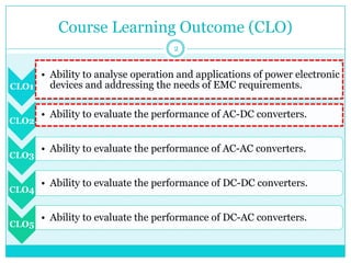
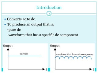
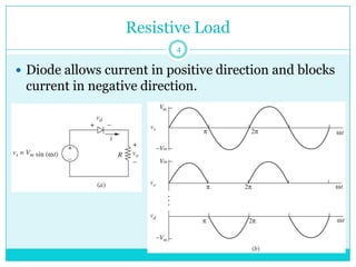
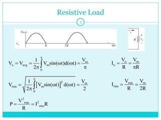
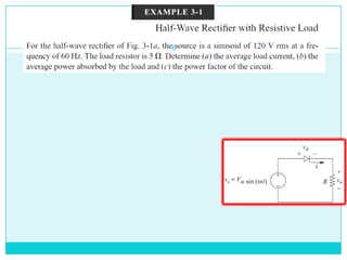
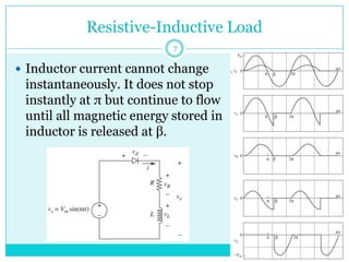
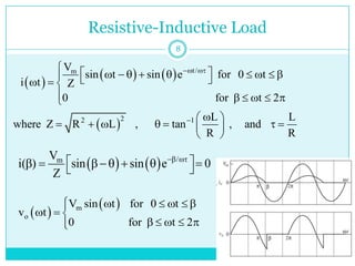
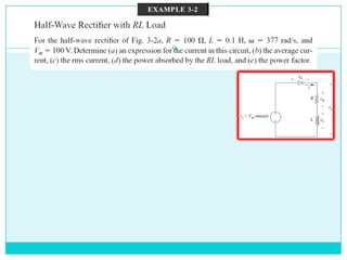
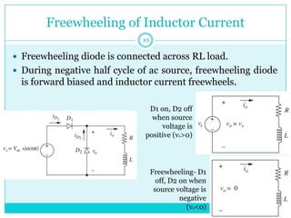
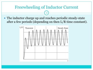
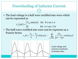
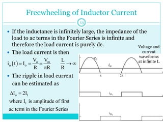
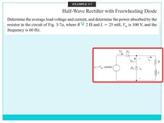
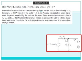
1. Half-Wave Rectifiers
PLT207 Power Electronics
1

2. Course Learning Outcome (CLO)
CLO1
• Ability to analyse operation and applications of power electronic
devices and addressing the needs of EMC requirements.
CLO2
• Ability to evaluate the performance of AC-DC converters.
CLO3
• Ability to evaluate the performance of AC-AC converters.
CLO4
• Ability to evaluate the performance of DC-DC converters.
CLO5
• Ability to evaluate the performance of DC-AC converters.
2

3. Introduction
 Converts ac to dc.
 To produce an output that is:
-pure dc
-waveform that has a specific dc component
pure dc waveform that has a dc component
3

4. Resistive Load
 Diode allows current in positive direction and blocks
current in negative direction.
4

5. Resistive Load
m
o avg m
0
V
1
V V V sin( t)d( t)
2

    
 

o m
o
V V
I
R R
 

 2 m
rms m
0
V
1
V V sin( t) d( t)
2 2

   
 
rms m
rms
V V
I
R 2R
 
2
2
rms
rms
V
P I R
R
 
5

6. 6

7. Resistive-Inductive Load
 Inductor current cannot change
instantaneously. It does not stop
instantly at π but continue to flow
until all magnetic energy stored in
inductor is released at β.
7

8. Resistive-Inductive Load
    /
m
V
i( ) sin sin e 0
Z
 
 
      
 
 
   
 
t/
m
2
2 1
V
sin t sin e for 0 t
i t Z
0 for t 2
L L
where Z R L , tan , and
R R
 

  
        
  
  
     


 
      
 
 
 
 
m
o
V sin t for 0 t
v t
0 for t 2
     

  
    


8

9. 9

10. Freewheeling of Inductor Current
 Freewheeling diode is connected across RL load.
 During negative half cycle of ac source, freewheeling diode
is forward biased and inductor current freewheels.
D1 on, D2 off
when source
voltage is
positive (vs>0)
Freewheeling- D1
off, D2 on when
source voltage is
negative
(vs<0)
10

11. Freewheeling of Inductor Current
 The inductor charge up and reaches periodic steady-state
after a few periods (depending on then L/R time constant).
11

12. Freewheeling of Inductor Current
 The load voltage is a half wave rectified sine wave which
can be expressed as
 The half-wave rectified sine wave can be expresses as a
Fourier Series
 
 
m
o
V sin t for 0 t
v t
0 for t 2
     

  
    


Load voltage and
current waveforms
at steady-state.
 
 
 
m m m
o 0 0
2
n 2,4,6...
V V 2V
v (t) sin t cos n t
2 n 1


    
  

12

13. Freewheeling of Inductor Current
 If the inductance is infinitely large, the impedance of the
load to ac terms in the Fourier Series is infinite and
therefore the load current is purely dc.
 The load current is then
 The ripple in load current
can be estimated as
  o m
o o
V V L
i t I
R R R
    

o 1
1
I 2I
where I is amplitude of first
ac term in the Fourier Series
 
Voltage and
current
waveforms
at infinite L
13

14. 14

15. 15

16. Controlled Half-Wave Rectifier
 The conduction of diodes are uncontrolled and therefore
the half-wave rectifiers analyzed previously are classified
as uncontrolled rectifiers.
 In uncontrolled rectifiers, the dc level of the output and
power transferred to the load are fixed once the source
and load parameters are established.
 To control the output of a half-wave rectifier, controllable
semiconductor switches can be used.
e.g. SCR: Conducts when,
1. SCR must be forward biased
2. current must be applied to the gate of SCR
16

17. Controlled Half-Wave Rectifier
Resistive load
 Load current starts
flowing at ωt=α and
stops at ωt=π.
 
 
m
o
V sin t for t
v t
0 for t 2
      

  
      


 
m
o
V
V 1 cos
2
  

m
rms
V sin(2 )
V 1
2 2
 
  
 
17

18. 18

19. Controlled Half-Wave Rectifier
RL load
 Load current starts flowing
at ωt=α and stops at ωt=β.
19

20. Controlled Half-Wave Rectifier
RL load
 Load current can be expressed as
 The extinction angle, β can be obtained by solving
 Output voltage can be expressed as
 
    ( t)/
m
V
sin t sin e for t
i t Z
0 otherwise
 
  
           
  
  


      ( )/
m
V
i 0 sin sin e
Z
 
 
         
 
 
 
m
o
V sin t for t
v t
0 for t 2
      

  
      


 
m
o
V
V cos cos
2
   

20

21. 21