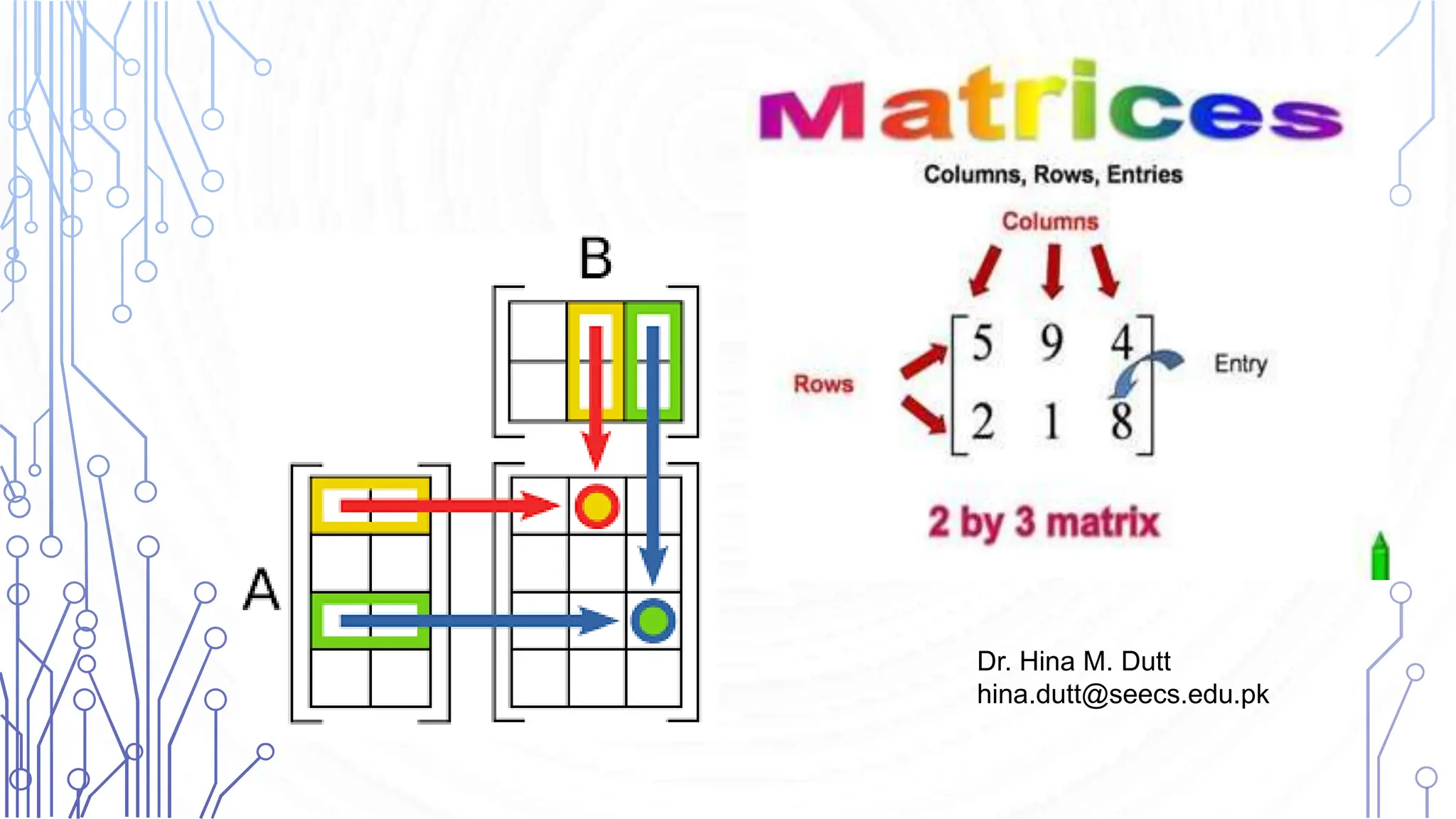
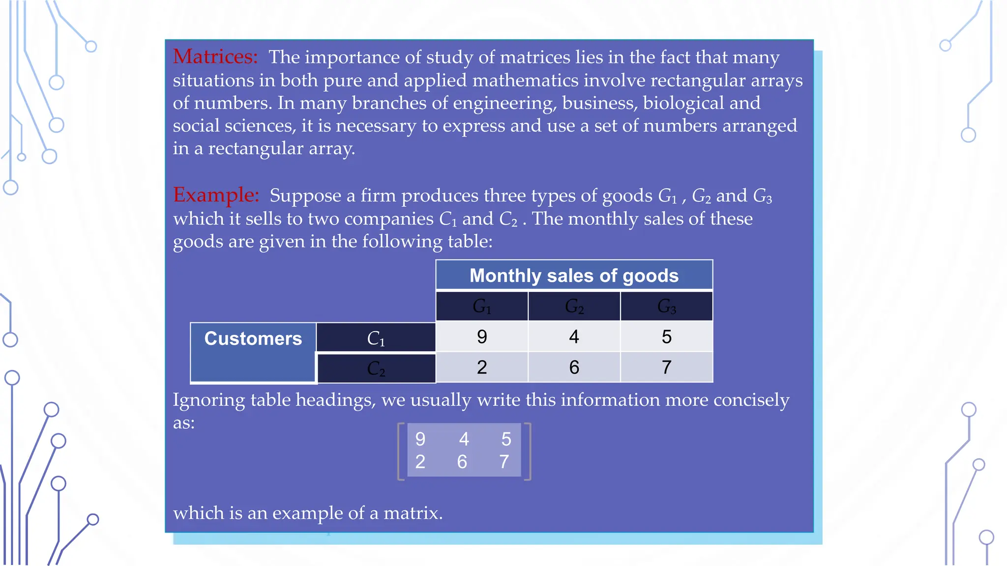
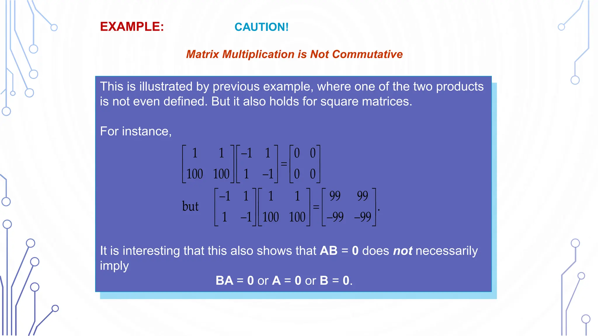
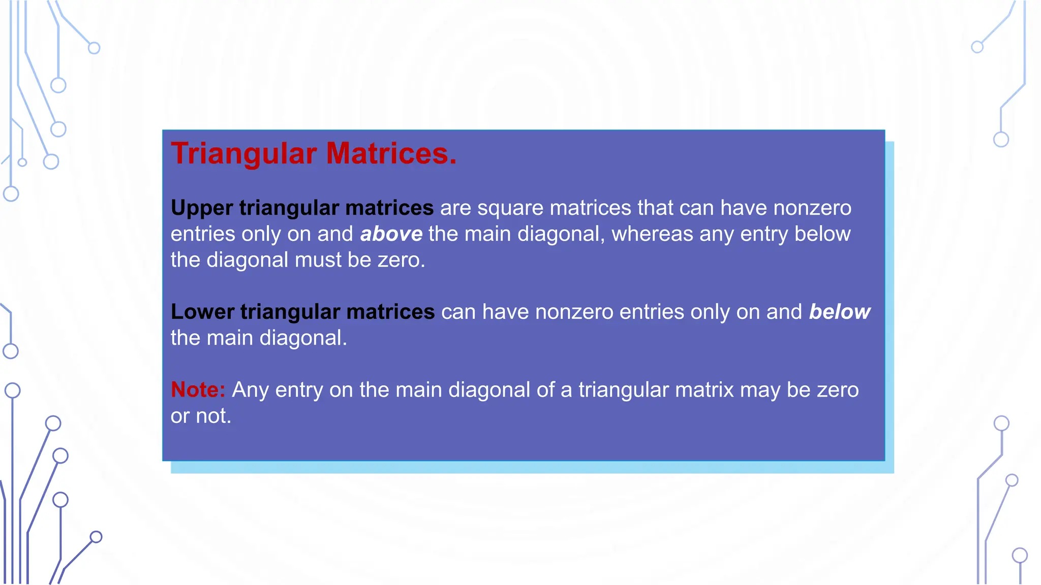
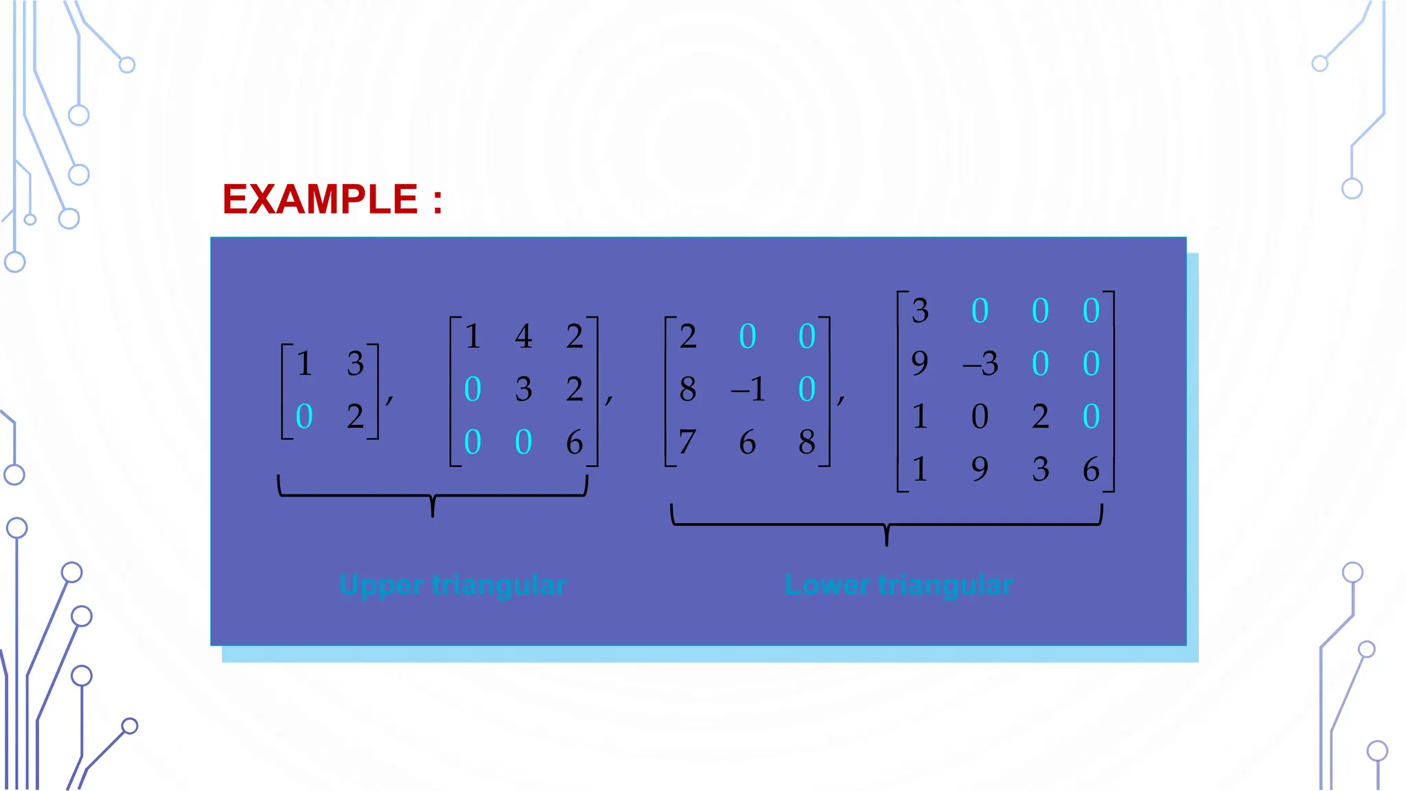
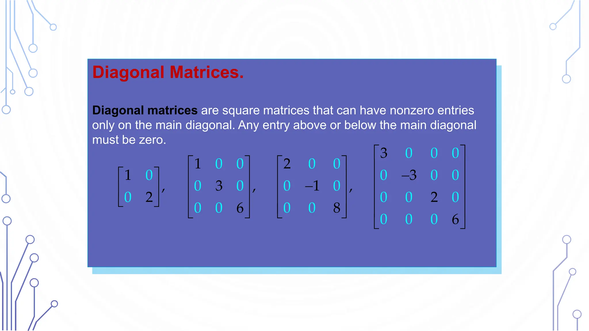
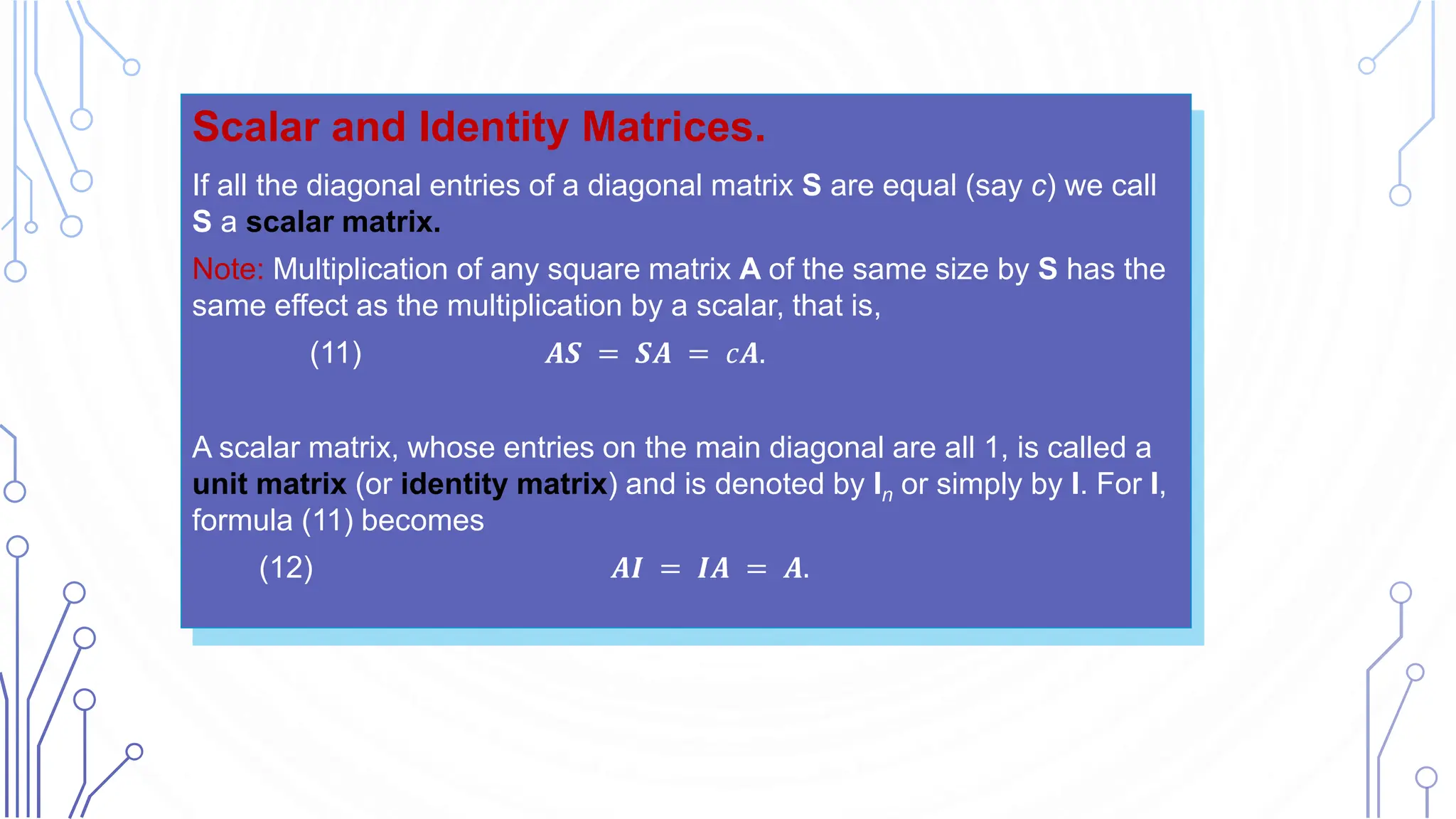
The document provides an introduction to matrices, highlighting their significance in various fields such as mathematics and engineering. It explains fundamental concepts including the definition, types, addition, and multiplication of matrices, along with notation and special categories like symmetric and diagonal matrices. The text emphasizes the importance of understanding matrix operations and their applicable rules, including the definitions of scalar multiplication and transposition.

1. Dr. Hina M. Dutt
hina.dutt@seecs.edu.pk

2. Introduction to Matrices

3. Matrices: The importance of study of matrices lies in the fact that many
situations in both pure and applied mathematics involve rectangular arrays
of numbers. In many branches of engineering, business, biological and
social sciences, it is necessary to express and use a set of numbers arranged
in a rectangular array.
Example: Suppose a firm produces three types of goods G₁ , G₂ and G₃
which it sells to two companies C₁ and C₂ . The monthly sales of these
goods are given in the following table:
Ignoring table headings, we usually write this information more concisely
as:
which is an example of a matrix.
Monthly sales of goods
G₁ G₂ G₃
9 4 5
2 6 7
Customers C₁
C₂
9 4 5
2 6 7

4. A matrix is a rectangular array of numbers or functions which we will enclose
in brackets. For example,
(1)
The numbers (or functions) are called entries or, less commonly, elements of the
matrix.
The first matrix in (1) has two rows, which are the horizontal lines of entries.
11 12 13
21 22 23
31 32 33
2
1 2 3
6
0.3 1 5
, ,
0 0.2 16
4
2
, , 1
4
2
x
x
a a a
a a a
a a a
e x
a a a
e x

 

   
   

   
 
 
   
 
     
   

5. Furthermore, it has three columns, which are the vertical lines of
entries.
The second and third matrices are square matrices, which means that
each has as many rows as columns—3 and 2, respectively.
The entries of the second matrix have two indices, signifying their
location within the matrix. The first index is the number of the row and
the second is the number of the column, so that together the entry’s
position is uniquely identified. For example, a23 (read a two three) is in
Row 2 and Column 3, etc.
The notation is standard and applies to all matrices, including those that
are not square.

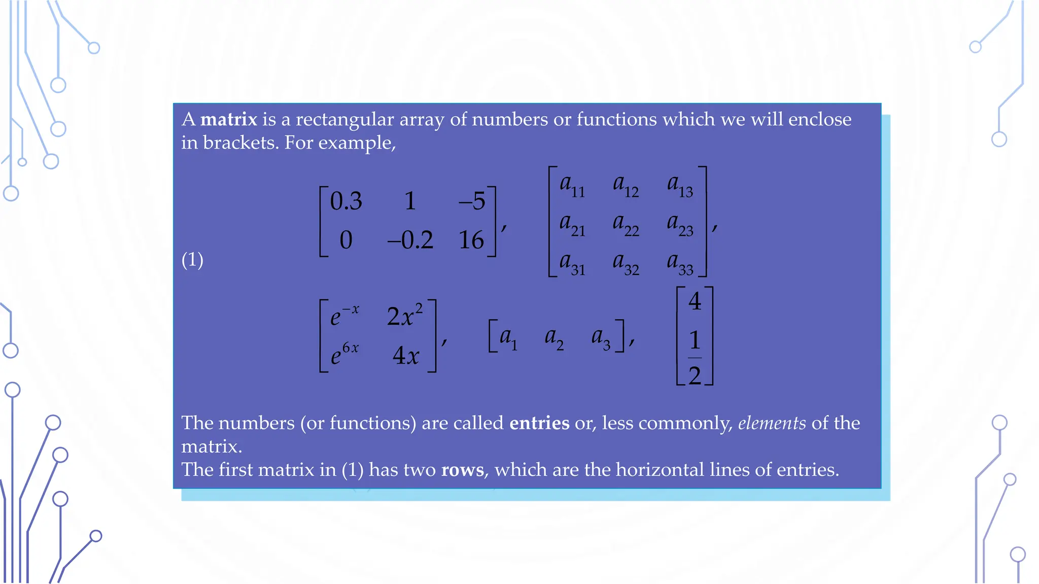
6. We shall denote matrices by capital boldface letters A, B, C, … , or by writing
the general entry in brackets; thus A = [ajk], and so on.
By an m × n matrix (read m by n matrix) we mean a matrix with m rows and n
columns—rows always come first! m × n is called the size of the matrix. Thus
an m × n matrix is of the form
(2)
General Concepts and Notations
11 12 1
21 22 2
1 2
.
n
n
jk
m m mn
a a a
a a a
a
a a a
 
 
 
 
 
   
  
 
 
A

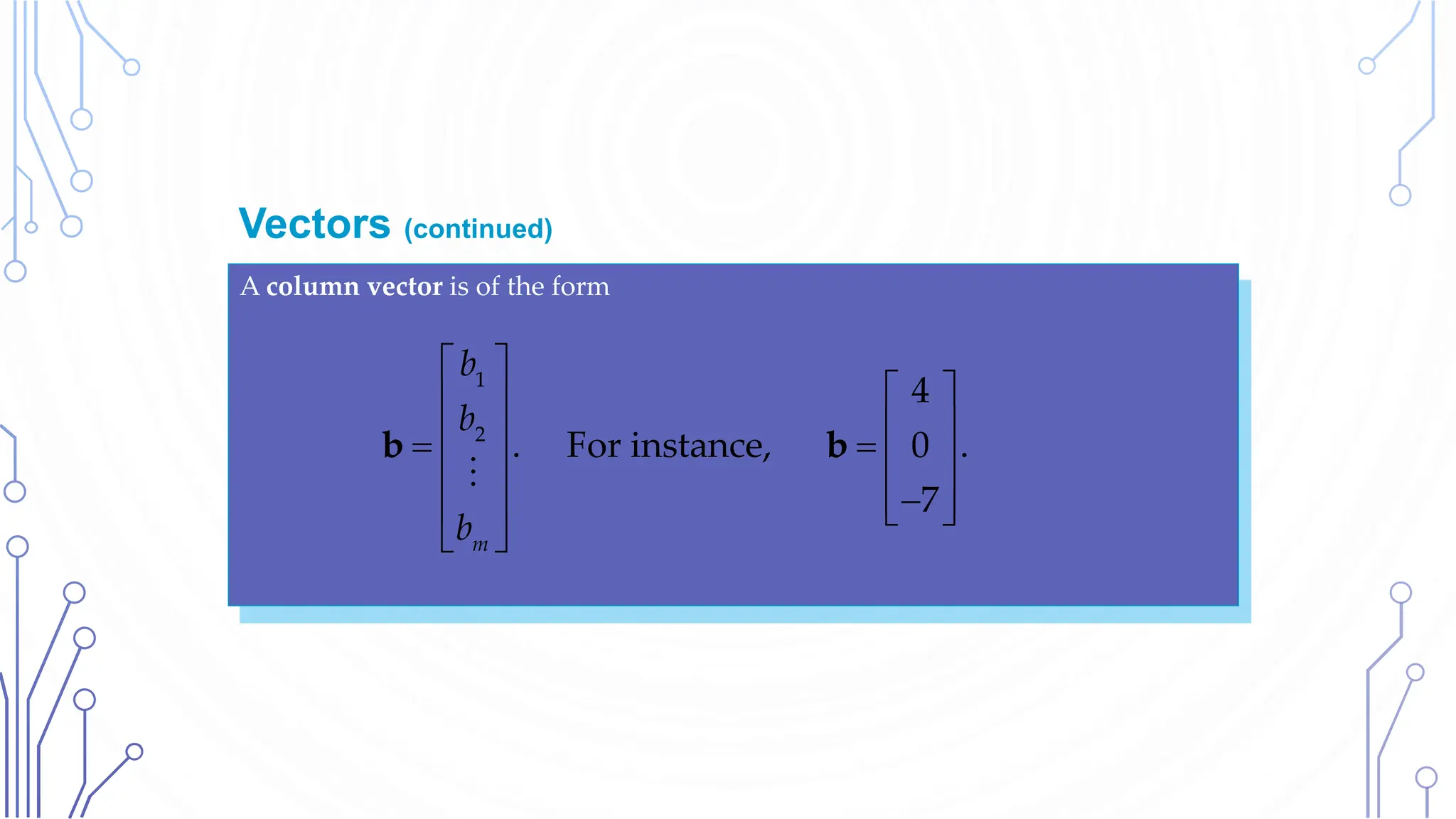
7. A vector is a matrix with only one row or column. Its entries are called the
components of the vector.
We shall denote vectors by lowercase boldface letters a, b, … or by its general
component in brackets, a = [aj], and so on.
Our special vectors in (1) suggest that a (general) row vector is of the form
Vectors
1 2
. For instance, 2 5 0.8 0 1 .
n
a a a
  
   
   
a a

8. A column vector is of the form
Vectors (continued)
 
 
 
 
 
   
 
 

   
 
1
2
4
. For instance, 0 .
7
m
b
b
b
b b

9. Equality of Matrices
Two matrices A = [ajk] and B = [bjk] are equal, written A = B, if and only if
(1) they have the same size
and
(2) the corresponding entries are equal ,
that is, a11 = b11, a12 = b12, and so on.
Matrices that are not equal are called different. Thus, matrices of different sizes
are always different.
Definition

10. Addition of Matrices
The sum of two matrices A = [ajk] and B = [bjk] of the same size is written as A + B
and has the entries ajk + bjk obtained by adding the corresponding entries of A and
B.
Note: Matrices of different sizes cannot be added.
Definition

11. Scalar Multiplication (Multiplication by a Number)
The product of any m × n matrix A = [ajk] and any scalar c (number c) is written as
“cA” and is the m × n matrix cA = [cajk] obtained by multiplying each entry of A by
c.
Definition

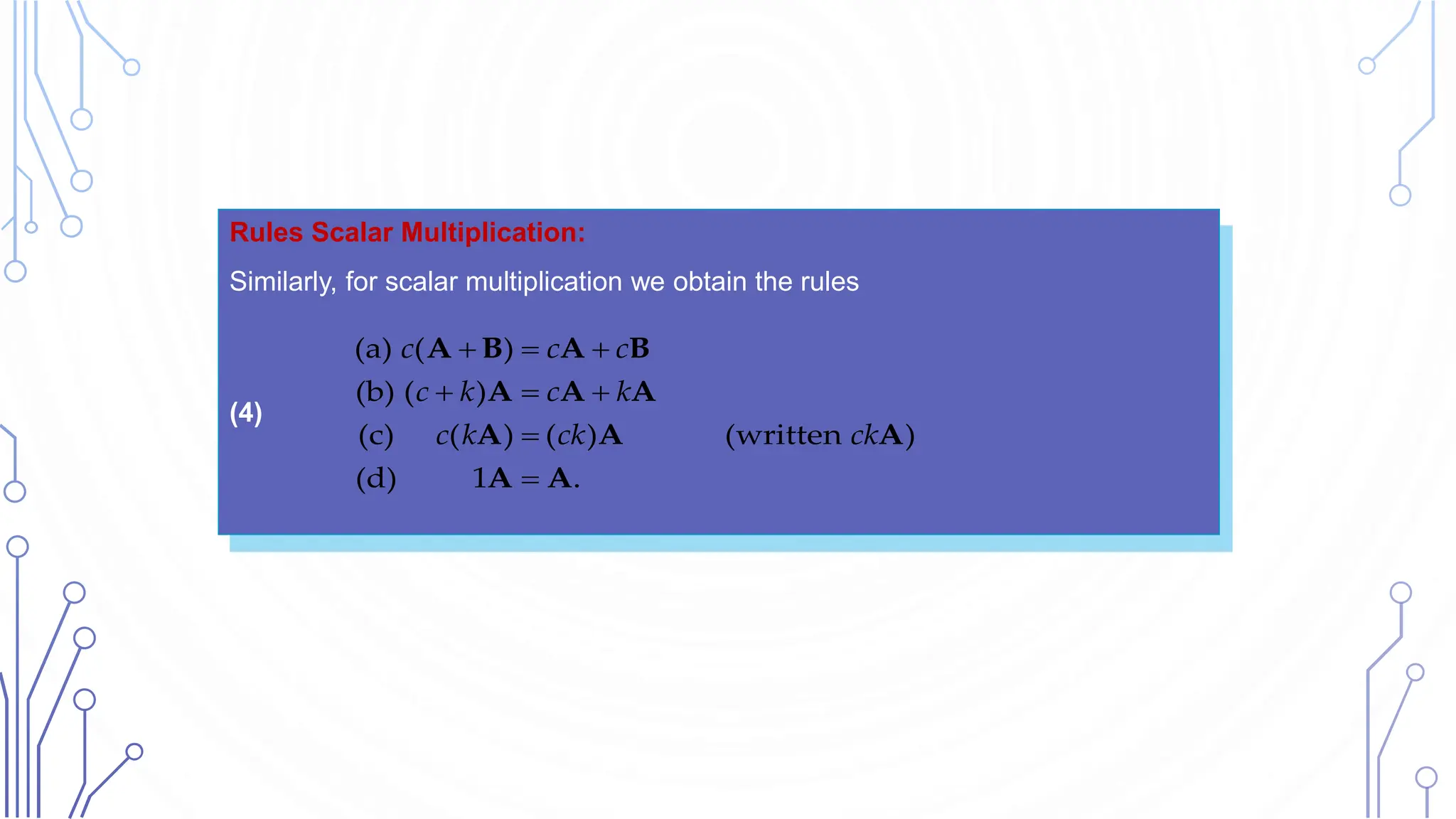
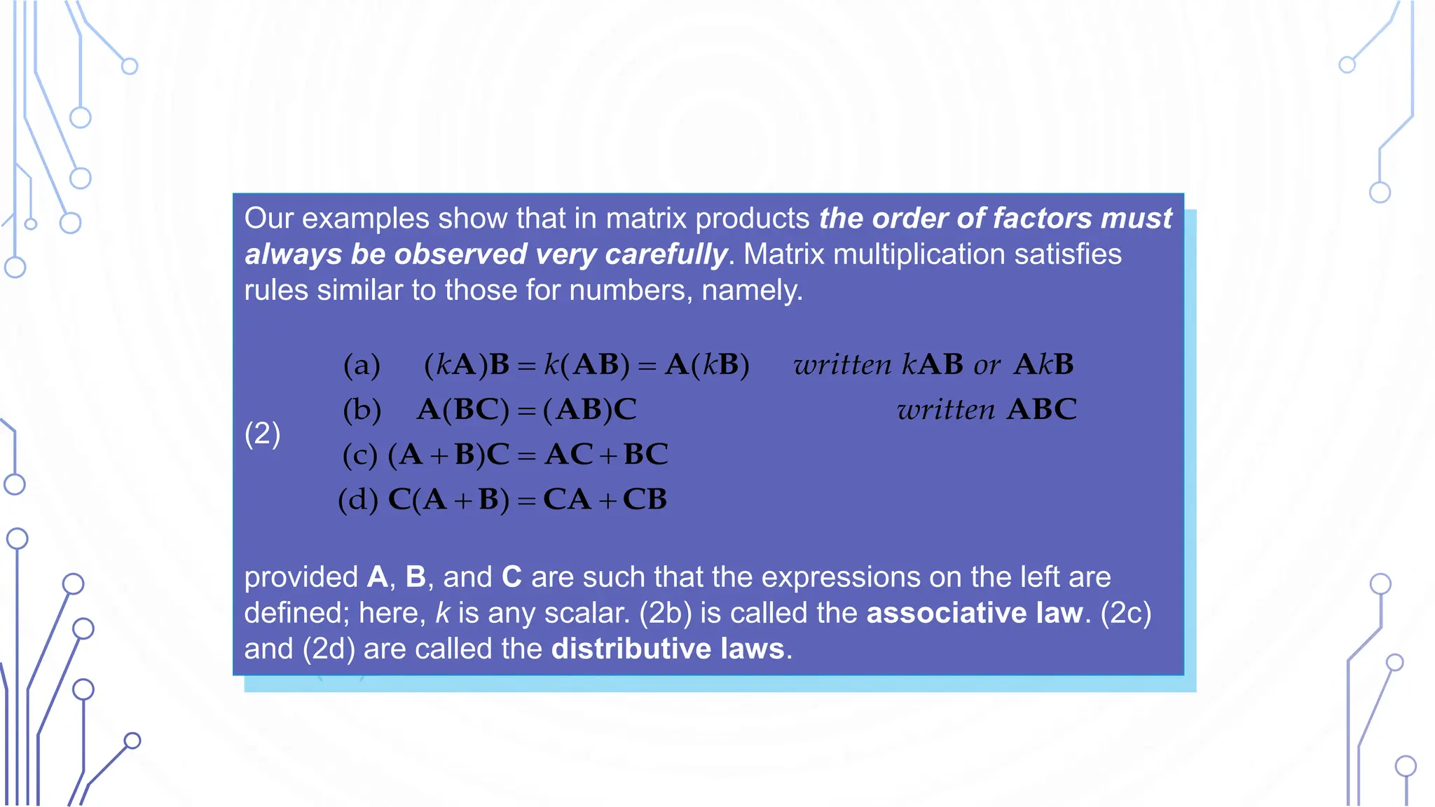
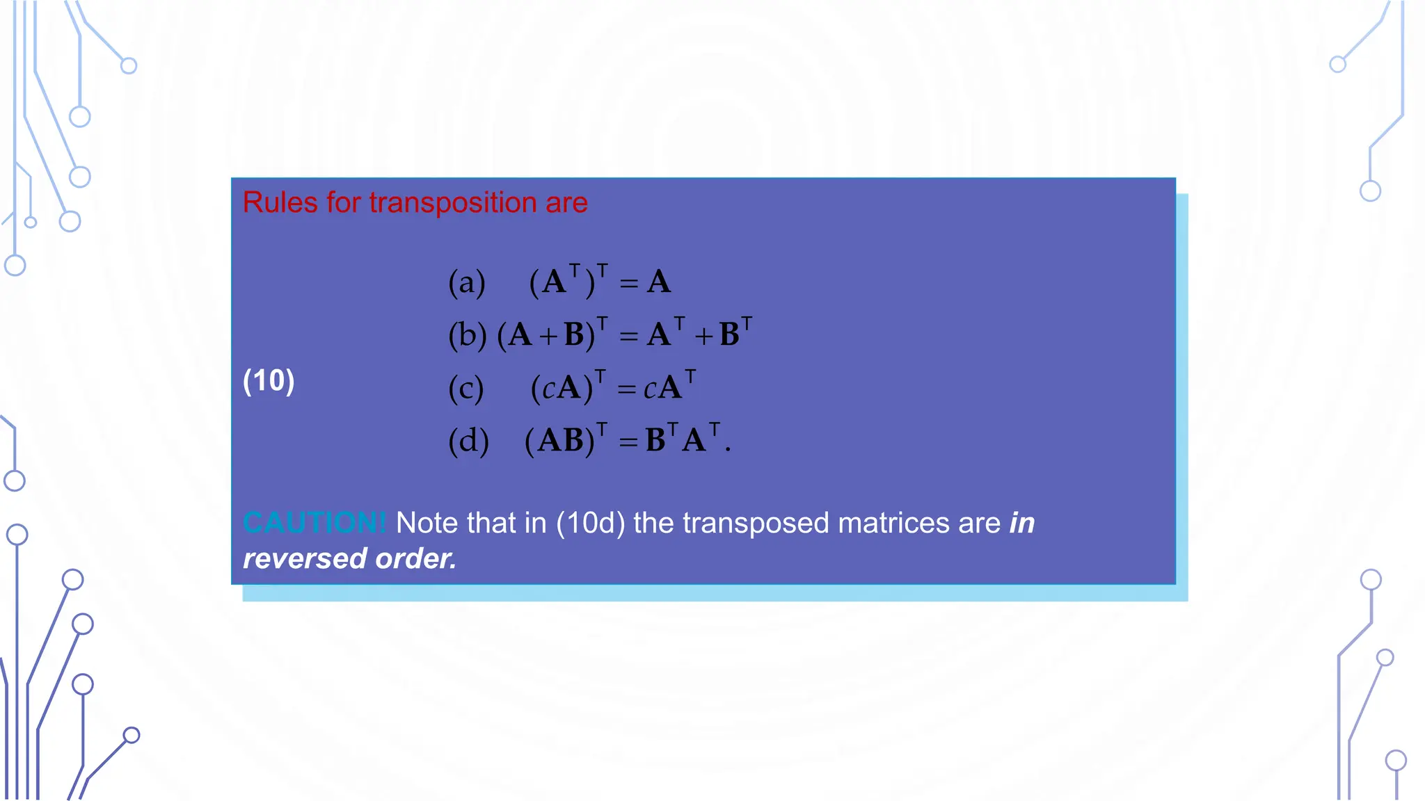
12. Rules for Matrix Addition:
From the familiar laws for the addition of numbers we obtain similar laws for the
addition of matrices of the same size m × n, namely,
(3)
Here 0 denotes the zero matrix or null matrix (of size m × n), that is, the m × n
matrix with all entries zero. Hence matrix addition is commutative and
associative [by (3a) and (3b)].
(a)
(b) ( ) ( ) (written )
(c)
(d) ( ) .
  
      
 
  
A B B A
A B C A B C A B C
A 0 A
A A 0

13. Rules Scalar Multiplication:
Similarly, for scalar multiplication we obtain the rules
(4)
(a) ( )
(b) ( )
(c) ( ) ( ) (written )
(d) 1 .
c c c
c k c k
c k ck ck
  
  


A B A B
A A A
A A A
A A

14. Matrix Multiplication
&
Laws of Transposition

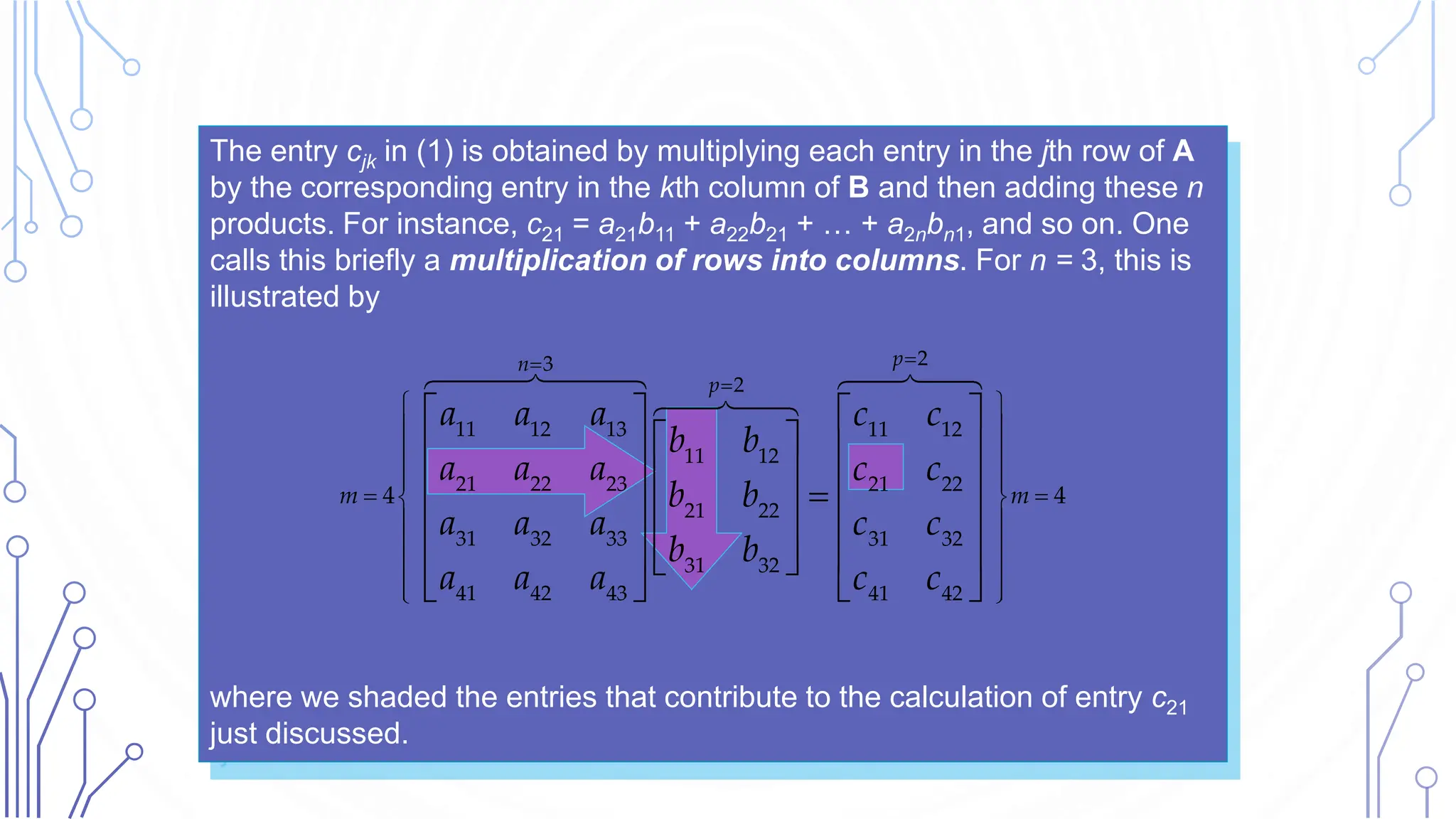
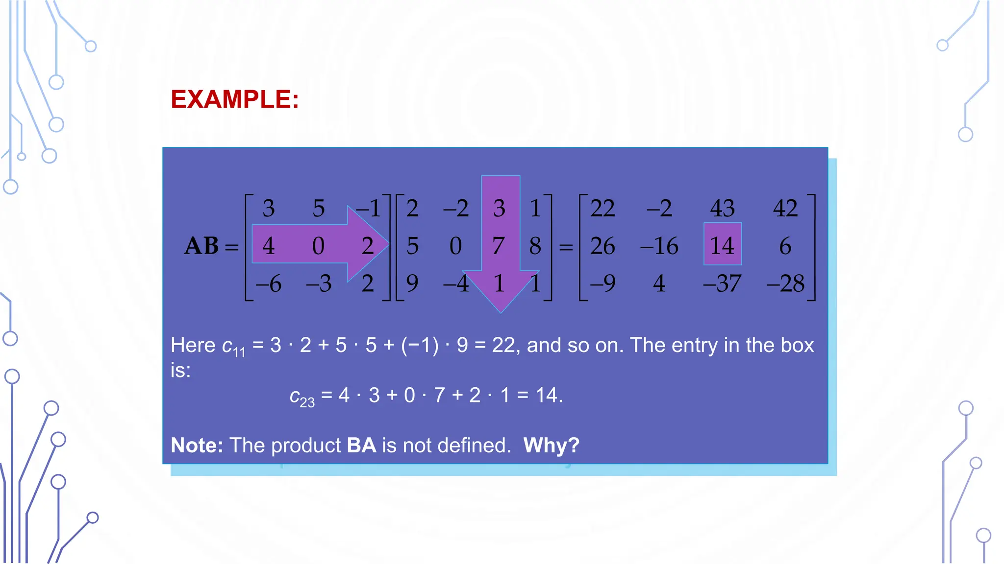
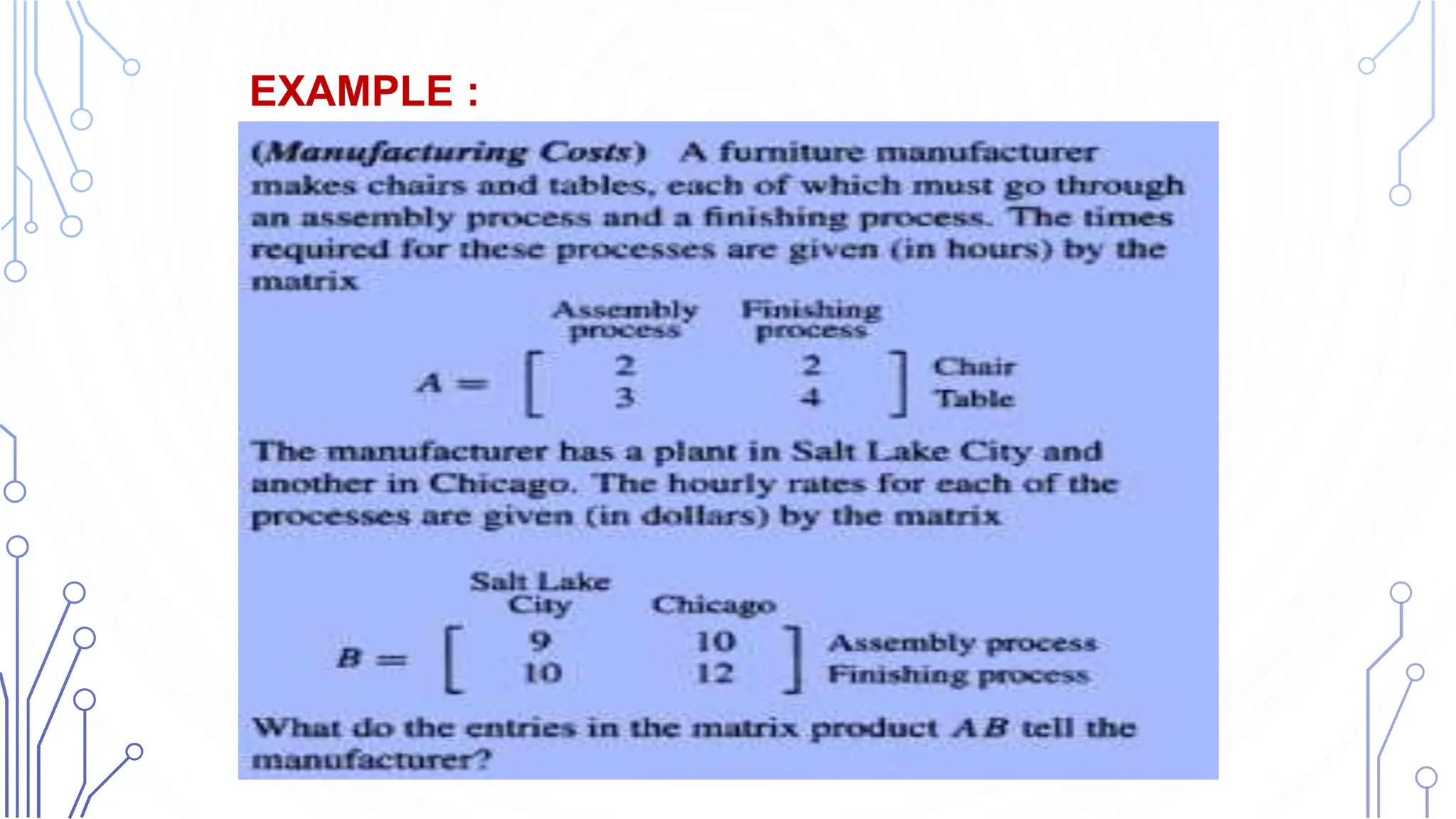
16. Multiplication of a Matrix by a Matrix
The product C = AB (in this order) of an m × n matrix A = [ajk] times an r
× p matrix B = [bjk] is defined if and only if r = n and is then the m × p
matrix C = [cjk] with entries
(1)
Definition: Matrix Multiplication
1 1 2 2
1
n
jk jl lk j k j k jn nk
l
c a b a b a b a b

    

1, ,
1, , .
j m
k p



17. The condition r = n means that the second factor, B, must have as many
rows as the first factor has columns, namely n.
A diagram of sizes that shows when matrix multiplication is possible is as
follows:
A B = C
[m × n] [n × p] = [m × p].

18. The entry cjk in (1) is obtained by multiplying each entry in the jth row of A
by the corresponding entry in the kth column of B and then adding these n
products. For instance, c21 = a21b11 + a22b21 + … + a2nbn1, and so on. One
calls this briefly a multiplication of rows into columns. For n = 3, this is
illustrated by
where we shaded the entries that contribute to the calculation of entry c21
just discussed.
4 4
m m
 
 
 
 
 
 
 
 
 
 
 
 
2
3
2
11 12 13 11 12
11 12
21 22 23 21 22
21 22
31 32 33 31 32
31 32
41 42 43 41 42
p
n
p
a a a c c
b b
a a a c c
b b
a a a c c
b b
a a a c c



   
 
   
 
   

 
   
 
   
 
 
 

19. Here c11 = 3 · 2 + 5 · 5 + (−1) · 9 = 22, and so on. The entry in the box
is:
c23 = 4 · 3 + 0 · 7 + 2 · 1 = 14.
Note: The product BA is not defined. Why?
EXAMPLE:
Matrix Multiplication
3 5 1 2 2 3 1 22 2 43 42
4 0 2 5 0 7 8 26 16 14 6
6 3 2 9 4 1 1 9 4 37 28
  
     
     
  
     
     
     
     
AB

20. This is illustrated by previous example, where one of the two products
is not even defined. But it also holds for square matrices.
For instance,
It is interesting that this also shows that AB = 0 does not necessarily
imply
BA = 0 or A = 0 or B = 0.
EXAMPLE: CAUTION!
Matrix Matrix Multiplication is Not Commutative,
AB ≠ BA in General
1 1 1 1 0 0
100 100 1 1 0 0
1 1 1 1 99 99
but .
1 1 100 100 99 99

    

    

    

    

    
  
    

21. Our examples show that in matrix products the order of factors must
always be observed very carefully. Matrix multiplication satisfies
rules similar to those for numbers, namely.
(2)
provided A, B, and C are such that the expressions on the left are
defined; here, k is any scalar. (2b) is called the associative law. (2c)
and (2d) are called the distributive laws.
(a) ( ) ( ) ( )
(b) ( ) ( )
(c) ( )
(d) ( )
k k k written k or k
written
 

  
  
A B AB A B AB A B
A BC AB C ABC
A B C AC BC
C A B CA CB

23. We obtain the transpose of a matrix by writing its rows as columns
(or equivalently its columns as rows).
This also applies to the transpose of vectors. Thus, a row vector
becomes a column vector and vice versa.
In addition, for square matrices, we can also “reflect” the elements
along the main diagonal, that is, interchange entries that are
symmetrically positioned with respect to the main diagonal to obtain
the transpose.
Hence a12 becomes a21, a31 becomes a13, and so forth.
Also note that, if A is the given matrix, then we denote its transpose
by AT.
Transposition

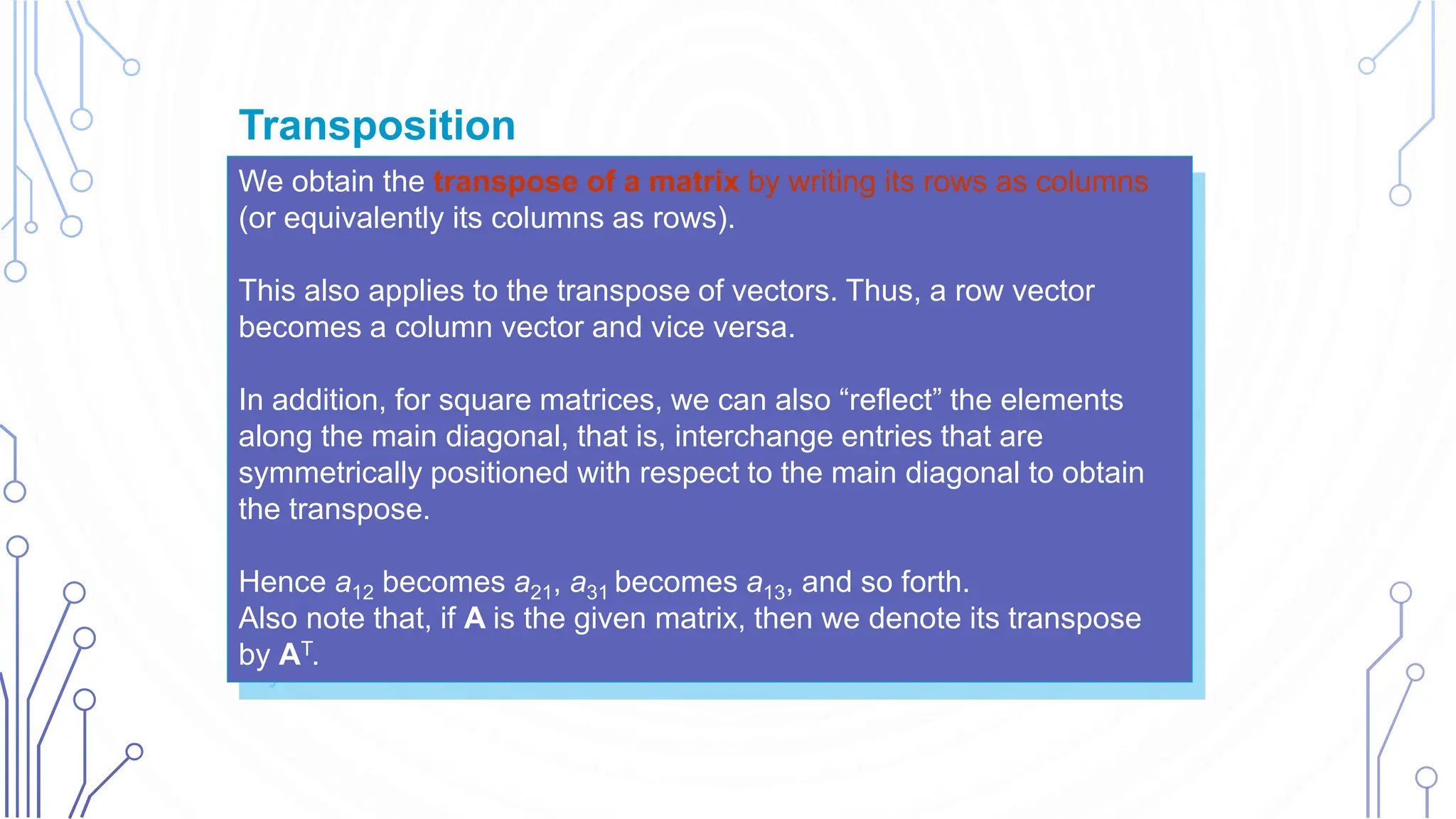
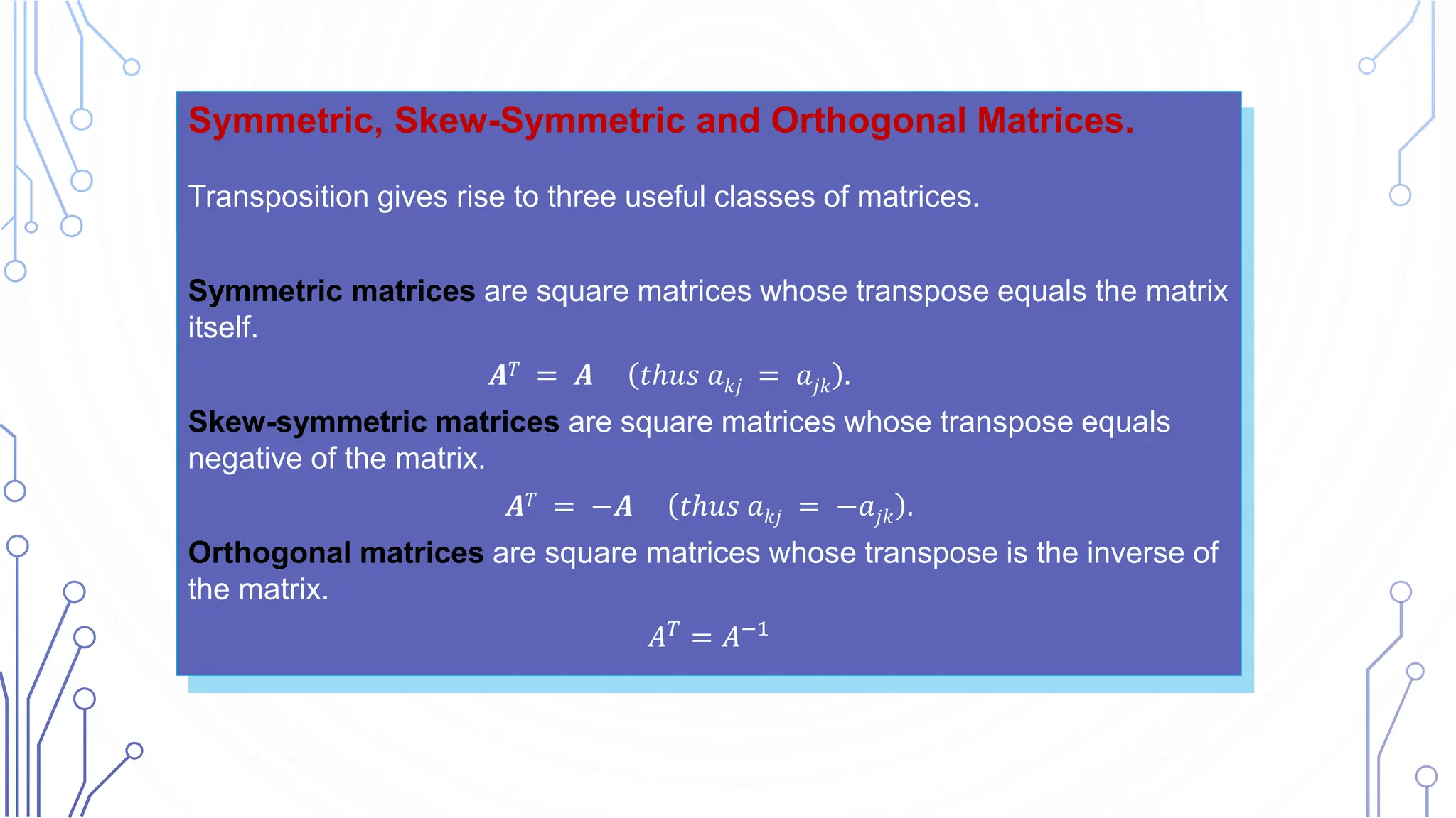
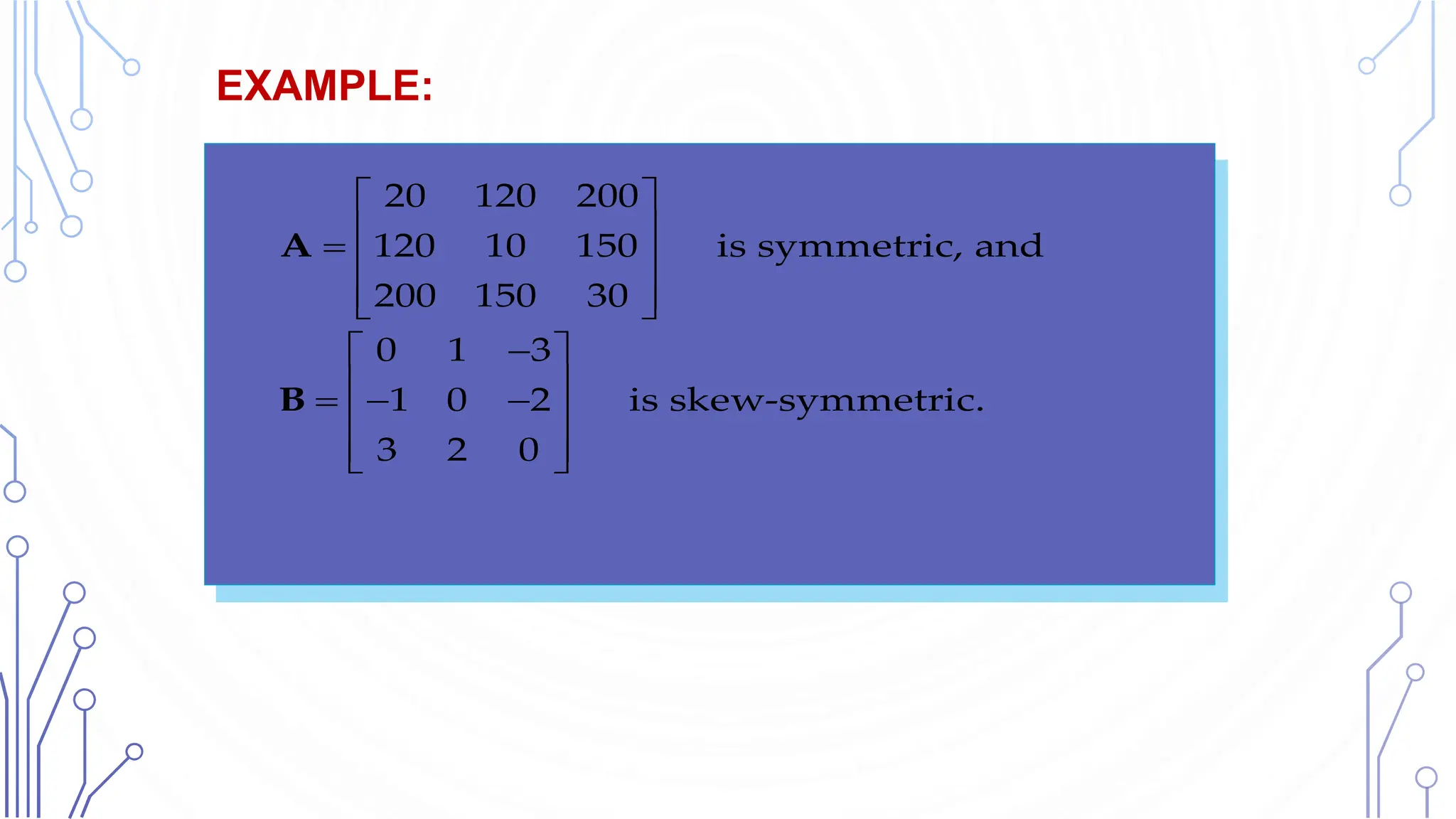
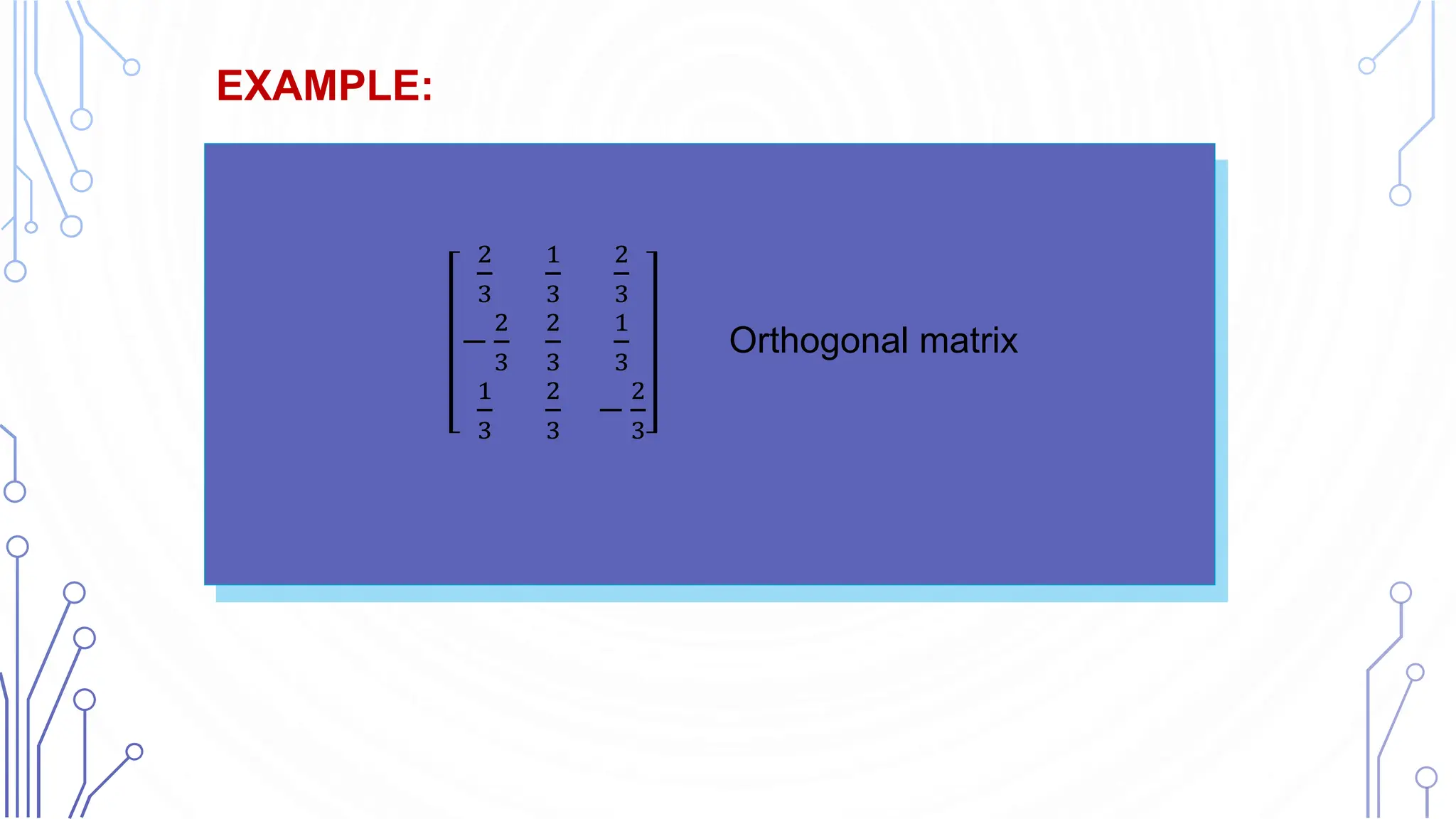
24. Transposition of Matrices and Vectors
The transpose of an m × n matrix A = [ajk] is the n × m matrix AT (read A
transpose) that has the first row of A as its first column, the second row of
A as its second column, and so on. Thus the transpose of A in (2) is AT =
[akj], written out
(9)
As a special case, transposition converts row vectors to column vectors
and conversely.
Definition
11 12 1
21 22 2
1 2
.
m
m
kj
n n mn
a a a
a a a
a
a a a
 
 
 
 
 
   
  
 
 
AT
a21
a12

25. Rules for transposition are
(10)
CAUTION! Note that in (10d) the transposed matrices are in
reversed order.

  


(a) ( )
(b) ( )
(c) ( )
(d) ( ) .
c c
A A
A B A B
A A
AB B A
T T
T T T
T T
T T T

26. SOME SPECIAL MATRICES

27. Symmetric, Skew-Symmetric and Orthogonal Matrices.
Transposition gives rise to three useful classes of matrices.
Symmetric matrices are square matrices whose transpose equals the matrix
itself.
𝑨𝑇 = 𝑨 𝑡ℎ𝑢𝑠 𝑎𝑘𝑗 = 𝑎𝑗𝑘 .
Skew-symmetric matrices are square matrices whose transpose equals
negative of the matrix.
𝑨𝑇 = −𝑨 𝑡ℎ𝑢𝑠 𝑎𝑘𝑗 = −𝑎𝑗𝑘 .
Orthogonal matrices are square matrices whose transpose is the inverse of
the matrix.
𝐴𝑇 = 𝐴−1

28. EXAMPLE:
Symmetric and Skew-Symmetric Matrices
20 120 200
120 10 150 is symmetric, and
200 150 30
0 1 3
1 0 2 is skew-symmetric.
3 2 0
 
 
  
 
 

 
 
  
 
 
 
A
B

29. EXAMPLE:
Symmetric and Skew-Symmetric Matrices
2
3
1
3
2
3
−
2
3
2
3
1
3
1
3
2
3
−
2
3
Orthogonal matrix

30. Triangular Matrices.
Upper triangular matrices are square matrices that can have nonzero
entries only on and above the main diagonal, whereas any entry below
the diagonal must be zero.
Lower triangular matrices can have nonzero entries only on and below
the main diagonal.
Note: Any entry on the main diagonal of a triangular matrix may be zero
or not.

31. Upper triangular Lower triangular
EXAMPLE :Und Lower Triangular Matrices
3
1 4 2 2
1 3 9 3
, 3 2 , 8 1 ,
2 1 0 2
6 7 6
0 0 0
0 0
0 0
0 0
0 0
8
1 9 3 6
0 0
 
     

       

       
       
   
 

32. Diagonal Matrices.
Diagonal matrices are square matrices that can have nonzero entries
only on the main diagonal. Any entry above or below the main diagonal
must be zero.
 
     

       

       
       
   
 
0 0 0
0 0 0 0
0 0 0 0
0 0 0 0
0 0 0 0
0 0 0
3
1 2
1 3
, 3 , 1 ,
2 2
6 8
0
6
0 0 0

33. Scalar and Identity Matrices.
If all the diagonal entries of a diagonal matrix S are equal (say c) we call
S a scalar matrix.
Note: Multiplication of any square matrix A of the same size by S has the
same effect as the multiplication by a scalar, that is,
(11) 𝑨𝑺 = 𝑺𝑨 = 𝑐𝑨.
A scalar matrix, whose entries on the main diagonal are all 1, is called a
unit matrix (or identity matrix) and is denoted by In or simply by I. For I,
formula (11) becomes
(12) 𝑨𝑰 = 𝑰𝑨 = 𝑨.

34. EXAMPLE :Und Lower Triangular Matrices
−3 0 0
0 −3 0
0 0 −3
,
𝑐 0 0
0 𝑐 0
0 0 𝑐
1 0 0
0 1 0
0 0 1
Scalar matrices
Identity matrix

35. Periodic Matrix.
A square matrix 𝐴 for which
𝐴𝑘+1
= 𝐴, 𝑘 being a positive integer ,
is called a Periodic matrix.
If k is the least positive integer for which 𝐴𝑘+1 = 𝐴, then 𝐴 is said to be of
period k.
If k = 1, so that 𝐴2 = 𝐴, then 𝐴 is called an Idempotent matrix.

36. EXAMPLE :Und Lower Triangular Matrices
 
 
 
 
 
 
 
 
   
   
   
  
   
   
   
   
 
 
 
  
 
 
 
 
2
2 2 4
1 3 4
1 2 3
2 2 4 2 2 4
1 3 4 1 3 4
1 2 3 1 2 3
2 2 4
1 3 4
1 2 3
A
A
A

37. EXAMPLE :Und Lower Triangular Matrices