2. 1336 J. Jarsj¨o et al.: Hydrological responses to climate change
fertilization, and pest control, which is associated with degra-
dation of environmental resources from salinization, contam-
ination, and water logging (Gordon et al., 2008; Johansson et
al., 2009; T¨ornqvist et al., 2011).
In order to realistically plan for land-use and water-use
changes, and efficiently mitigate the adverse effects of such
changes, processes need to be understood and quantified on
the drainage basin scale. This is best done within hydro-
logical basins, because the topographical water divides that
define these basins are physical boundaries that reasonably
well delimit the flows of water and water-borne substances
through the landscape, and the environmental impacts of
man-made changes to these flows. Existence of large aquifer
systems means that groundwater flows may extend over
larger hydrological units than surface water basins. However,
these subsurface flow effects decrease with increasing basin
scale and can in many cases be investigated and quantified
by state-of-the-art hydrogeological methods. The increasing
hydrological impacts of climate change (Milly et al., 2005;
Groves et al., 2008; Bengtsson, 2010) constitute a greater
quantification challenge, with several open scientific ques-
tions in need of further investigation, not least regarding the
large spatial scale discrepancy between a typical drainage
basin and its hydrological modeling, and the global scale
and coarse resolution of general circulation models (GCMs)
(Milly et al., 2005; Groves et al., 2008).
Regionally, the impacts on water resources from changes
in global atmospheric circulation and climate overlap with
the impacts from land-use and water-use changes (Lobell
and Field, 2007). For instance, in arid and semi-arid re-
gions, water availability critically limits water-demanding
agricultural expansion and economic growth, making such
regions particularly vulnerable to impacts of expected fu-
ture climate changes (IPCC, 2007). The different overlapping
causes of freshwater resource changes make it hard to dis-
tinguish between various hydrological cause-effect relations
and impacts (Milly et al., 2002; Piao et al., 2007; Destouni
et al., 2008). However, for all water resource changes that
are driven by different types of change at the surface of a
hydrological basin, hydro-climatic change projections can
be considerably improved by honoring and accounting for
the water flux bounds implied by the basic basin-scale wa-
ter balance equation ET = P − R − S. Such bounds on the
commonly difficult to measure and quantify vapour flux by
evapotranspiration (ET) at the land surface can then be de-
rived on basin scales from directly measured and/or model-
interpreted data on precipitation (P) at the basin surface,
runoff (R) at the basin outlet, and storage change ( S) within
the basin (Shibuo et al., 2007; Asokan et al., 2010; Destouni
et al., 2010; T¨ornqvist and Jarsj¨o, 2012). Without such condi-
tioning to water balance components, the Penman-Monteith
type of evapotranspiration (ET) models can yield errors of
30 % to 50 % (Kite and Droogers, 2000), which is consider-
ably larger than the errors of 10 % to 15 % that are involved
in ET estimation from water balance closure (Asokan et al.,
2010).
In this paper, we use and extend (from previous related
studies of historic hydro-climatic change; Shibuo et al., 2007;
Alekseeva et al., 2009; Destouni et al., 2010; T¨ornqvist and
Jarsj¨o, 2012) such a basin-scale water balance approach to in-
vestigate future hydrological responses to projected climate
change at the land surface of a hydrological basin. This is
done by linking the projections of basin-scale surface cli-
mate change from 20 different GCMs with already devel-
oped hydrological modeling (based on the above-cited his-
toric hydro-climatic change studies and data) for the example
case of the closed and intensely irrigated Aral Sea Drainage
Basin (ASDB) in Central Asia. We specifically analyze sur-
face boundary-driven, multi-decadal hydrological changes,
following the historic 20th century development of approx-
imately 8 million hectares of irrigated land in the ASDB.
The ASDB is one of the world’s largest hydrological basins
and is spatially well resolved by current GCMs. Further-
more, the dramatic Aral Sea shrinkage over the last 60 yr
constitutes a great amplifier of different water change sig-
nals, which has been used in previous water balance-based
studies of the ASDB to understand and resolve the historic
impacts of different hydro-climatic change drivers in this
basin. A main question investigated here is then to what ex-
tent, and how, future climate change can interact with the
human re-distributions of water in modifying future water
fluxes and impacting future water resource availability. Such
interactions with local-regional water resource management
are not well resolved in current GCMs, or in regional climate
models (RCMs). To complement such large-scale modeling,
the present basin-scale water balance approach can explic-
itly consider and account for how various hydrological flows,
such as ET, are limited by actual basin-scale human water
and resulting water availability. We also investigate and pro-
vide example quantifications of main uncertainties in such
modeling of hydrological responses to multi-GCM projec-
tions of future basin-scale climate change.
2 Study area and historic hydro-climatic change
With its total area of 1 870 000 km2, the ASDB occupies
1.3 % of the Earth’s land surface, and by its traditional def-
inition, almost the entire region of Central Asia (Fig. 1).
Records of hydrological responses to the historic changes
in surface boundary conditions show that, despite a P in-
crease from the beginning of the 20th century (Fig. 1), the
discharge (Q) into the Aral Sea, through the principal rivers
of Amu Darya and Syr Darya in the ASDB, has decreased
from the pre-1950 value of about 60 km3 yr−1 to today’s
average of less than 10 km3 yr−1 (Fig. 1; Mamatov, 2003;
Jarsj¨o and Destouni, 2004; Shibuo et al., 2007; Destouni et
al., 2010). Such a Q decrease may in principle be associated
with a corresponding increase in the water vapor flux to the
Hydrol. Earth Syst. Sci., 16, 1335–1347, 2012 www.hydrol-earth-syst-sci.net/16/1335/2012/
3. J. Jarsj¨o et al.: Hydrological responses to climate change 1337
0
20
40
60
80
1900 1920 1940 1960 1980 2000 2020 2040
Riverdischarge(km3yr-1)
Year
Average discharge:
pre-irrigation period
1901-1950
8.1
9.6
7.9
9.4
4
6
8
10
12
14
1900 1920 1940 1960 1980 2000 2020
Year
Temperature(
o
C)
Observed
Running average, 30yr
Ensemble mean, uncal
Ensemble mean, calib
CSIRO
ECHAM4
GFDL99
HADCM3
NIES99
CNCM3
ECHOG
#X #Y
#X #Y
353
363
267
257
100
200
300
400
500
1900 1920 1940 1960 1980 2000 2020
Year
Precipitation(mmyr
-1
)
GIER
HADGEM
INCM3
IPCM4
MRCGCM
NCCCSM
NCPCM
a
b
c
not bias corr.
bias corr.
9.4
9.6
8.1
7.9
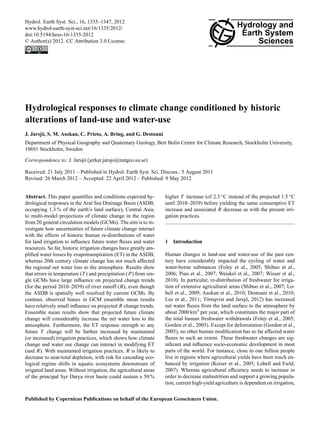
Fig. 1. Trends in (a) observed (grey line; running average in black) and projected (14 AR4 GCMs; colored thin lines) temperature T ,
(b) observed and projected precipitation P , and (c) observed river discharge R at outlets, for the ASDB. Thick red lines show ensemble mean
values of the GCM projections, and thick, blue lines show ensemble mean changes ( T and P ) from the observed mean conditions of the
reference period 1961–1990. Insert map shows the extent and location of the ASDB (grey area), its irrigated land (green areas), the Aral Sea
in 1960 (light blue) and in 2010 (dark blue), and the principal Amu Darya and Syr Darya rivers (blue).
atmosphere through ET, or in the groundwater recharge and
associated diffuse groundwater discharges (DD) to the Aral
Sea, or some combination of both. The fate of the missing
water associated with a decrease in river discharge Q must
be estimated independently in order to resolve how much of
the so far observed Q change reflects an ET change, and how
much should be attributed to a DD change.
In the ASDB, all diffuse groundwater flow converges into
the terminal Aral Sea, contributing to its water level, which
has decreased by 25 m since the 1960’s. Detailed previous
water balance studies with a coupled groundwater-seawater
model and independent analyses of groundwater hydraulics
have shown that this decrease is incompatible with large in-
creases in DD (Jarsj¨o and Destouni, 2004; Shibuo et al.,
2006; Alekseeva et al., 2009). Since the historic changes in
DD are much smaller than the observed historic Q changes
in the ASDB, the latter must be due to ET changes of corre-
sponding magnitude. Previously reported ASDB results have
further shown that the ET losses associated with the his-
toric, post-1950 temperature (T ) increase of 1 ◦C (Fig. 1a)
are smaller than the historic water gains from increased P
(Fig. 1b), and that the drying of ASDB rivers (Q decrease;
www.hydrol-earth-syst-sci.net/16/1335/2012/ Hydrol. Earth Syst. Sci., 16, 1335–1347, 2012
4. 1338 J. Jarsj¨o et al.: Hydrological responses to climate change
Fig. 1c) and associated major Aral Sea shrinkage have not
so far been driven by the observed historic surface climate
change within the ASDB (Shibuo et al., 2007).
3 Future hydro-climatic change projections
We consider future climate change scenarios for the ASDB
(Fig. 1) by using the spatially distributed outputs for this
basin from 20 General Circulation Models (GCMs). These
comprise all available GCMs in the third and fourth assess-
ment reports (TAR and AR4, respectively; Greenhouse Gas
Emission Scenario A2a) of the Intergovernmental Panel of
Climate Change (IPCC) (IPCC, 2007), from which both T
and P output is available. As the ASDB extends over a con-
siderable number of grid cells (29 ± 23) of the considered
GCMs (Table 1), the GCM spatial resolution biases should
be small (Wood et al., 2004; Milly et al., 2005; Mujumdar
and Ghosh, 2008), justifying hydrological impact studies by
direct use of GCM projection results for basins of this size.
(Milly et al., 2002; Palmer and R¨ais¨anen, 2002).
3.1 Catchment delineation and hydrological modeling
steps
The hydrological modeling considered here is spatially dis-
tributed, using the water module of the PCRaster-based
Polflow model (De Wit, 2001), similar to previous inves-
tigations of historic hydro-climatic variability and change,
specifically for the ASDB (Shibuo et al., 2007) as well as for
other drainage basins in different parts of the world (Darracq
et al., 2005; Jarsj¨o et al., 2008; Darracq and Destouni, 2009;
Asokan et al., 2010). As input for the hydrological modeling
module in PCRaster/PolFlow, each of the 9 million cells of
the hydrological grid was assigned properties of ground slope
and slope direction (based on the SRTM data), precipitation
P and temperature T (30-yr average) from GCM output or
observational data from the Climate Research Unit (CRU)
TS 2.1 database (Mitchell and Jones, 2005), land use (clas-
sified as irrigated or not irrigated, from the Global Map of
Irrigated Areas; Siebert et al., 2005), and land cover (classi-
fying river water and reservoir grid cells, after Danko, 1992,
and Johansson et al., 2009). The ground-slope and slope di-
rection inputs were pre-processed using Shuttle Radar To-
pography Mission (SRTM) data (Farr et al., 2007), isobath
data from Alekseeva et al. (2009), and stream location data
from the Digital Chart of the World (Danko, 1992), associ-
ating each grid cell with a unique slope and flow direction
(N, NE, E, S, SW, W, or E, for a grid that is oriented in the
N–S and E–W directions), into the neighbouring cell with
the lowest elevation. Using PCRaster/PolFlow routines (De
Wit, 2001), a topography-driven flow accumulation network
of the ASDB was constructed by associating a sub-catchment
area i to each grid cell i, including all upstream cells that
contribute to the flow through the cell, on the basis of all
Table 1. Number of grid cells within the ASDB for the considered
GCMs of IPCCs AR4 and TAR. The IDs of the GCMs are given as
in the GCM summary by Solomon et al. (2007).
ID of GCM Version Number of grid
cells within ASDB
CSIRO-CSMK3 AR4 54
ECHAM5-MPEH5 AR4 56
GFDL-GFCM 20 21 AR4 37
HADCM3 AR4 20
NIES-MIMR AR4 24
CNCM3 AR4 24
ECHOG AR4 15
GIER AR4 11
HADGEM AR4 68
INCM3 AR4 7
IPCM4 AR4 19
MRCGCM AR4 23
NCCCSM AR4 99
NCPCM AR4 23
CSIRO-MK2 TAR 11
ECHAM4 TAR 26
GFDL99-R30 TAR 24
HADCM3 TAR 20
CCSR/NIES TAR 6
CCCma-CGCM2 TAR 16
upstream defined flow directions. Furthermore, for each cell,
the locally created average precipitation surplus, PS, was cal-
culated as P − ET, in which the evapotranspiration (ET) was
given according to Eqs. (1) to (7). Based on the calculated PS
and the flow accumulation network, the total river discharge
(Q) and total runoff (R) leaving a grid cell was finally ob-
tained from the network-routed sum of PS.
In this way, the model can quantify the three principal out-
flow components of lake drainage basins, namely the dis-
charges of the principal rivers into the lake (given in the
model by Q at the river outlet points at the Aral Sea), the dif-
fuse flows along the shoreline of the lake (from groundwater
and small, transient streams; given in the model by the sum
of R along the Aral Sea coastline), and ET over the land and
water surfaces of the lake drainage basin (given in the model
by the sum of actual ET over the basin’s land surfaces and po-
tential ET (ETp) over the basin’s water surfaces). The annual
mean ET (actual evapotranspiration) was estimated from the
ETp (potential evapotranspiration) according to Turc (1954):
ET =
P
0.9 + P2
ET2
p
(1)
where ET, ETp, and P are expressed in mm yr−1, and
ETp was estimated as a function of T according to Lang-
bein (1949):
ETp = 325 + 21 · T + 0.9 · T 2
(2)
Hydrol. Earth Syst. Sci., 16, 1335–1347, 2012 www.hydrol-earth-syst-sci.net/16/1335/2012/
5. J. Jarsj¨o et al.: Hydrological responses to climate change 1339
where T is expressed in ◦C. In the present as in previously re-
ported results from distributed hydrological modeling of the
ASDB (Destouni et al., 2010; Shibuo et al., 2007) and else-
where (Asokan et al., 2010), irrigation has been handled by
spreading the known water diversions from rivers (currently
50 km3 yr−1 from the ASDB rivers) over the known irrigated
areas in the basin (from Siebert et al., 2005). More specif-
ically, the superficial nature of the irrigation in the ASDB,
which is dominated by furrow irrigation, was considered by
adding the diverted water as extra P over the irrigated fields,
hence keeping them in a wetter state than prescribed by the
P-data of CRU. This means that the water application of
50 km3 yr−1 is an input to the model, whereas the associated
water loss (i.e. consumptive water use) by contrast is an out-
put, determined by the modeled amount of irrigation water
(extra P) that remains in the basin after losses to the atmo-
sphere through ET. The water diversions for agriculture con-
sidered here have constituted approximately 90 % of the total
water diversions of ASDB, since at least the 1960’s. More-
over, in comparison with water diversions for other sectors
such as the industrial and the municipal ones, the agricultural
diversions can result in actual water consumption (i.e. physi-
cal loss of water from the surface of the basin) to a relatively
large extent, due to the above-mentioned superficial nature
of irrigation, which makes the diverted water relatively avail-
able for ET.
If the actual ET (ETact) of the ASDB for a given histor-
ical period were known from direct measurements, the per-
formance of the adopted Langbein-Turc ET method (Eqs. 1
and 2) could be evaluated by determining a factor X that
quantifies how much the modeled, total ET over the basin
(ETmod) differs from the actual ET (ETact):
ETact = X · ETmod (3)
in which the factor X equals unity for the case that the
modeled ET independently reproduces ETact. However, since
ETact cannot be obtained from direct measurements at basin
scales, we estimate here X from available observations of to-
tal precipitation over the drainage basin, Pobs (Fig. 1b), and
total river discharge Qobs at the outlet of the drainage basin
(Fig. 1c), according to the expression of Jarsj¨o et al. (2008):
X =
Qobs
Qmod
+ 1 −
Qobs
Qmod
·
Pobs
ETmod
(4)
in which Qmod is the modeled total river discharge at the
basin outlet, and all the variables to the right of the equal
sign have units of volume per time. In Eq. (4), the value of X
represents a bias-factor by which the modeled total ET would
need to be scaled, in order to obtain a calibrated model that
reproduces the observed river discharge Qobs. The factor X
equals unity if there is no bias, i.e. if the model independently
can reproduce Qobs without any scaling of ETmod.
Considering also future hydro-climatic projections, the
performance of the adopted Langbein-Turc ET method
(Eqs. 1 and 2) is compared with the Thorntwaite (1948)
method that uses monthly climate data as input and therefore
explicitly accounts for seasonal variations:
ETp = 16 ·
tdi
30
·
Ni
12
· 10 ·
Ti
I
α
(5)
in which tdi is the total number of days over which ETp is
calculated, Ni is the average day length in hours for month i,
Ti is the average temperature (◦C) for month i (equals zero if
the temperature is negative), and I and α are given by:
I =
12
i=1
(0.2 · Ti)1.514
(6)
α= 6.75 · 10−7
I3
− 7.71 · 10−5
· I2
+ 1.79 · 10−2
· I + 0.49. (7)
The day lengths Ni for ASDB were obtained from compu-
tations based on Meeus (1991), averaging the day lengths at
latitude 40 and 45.
3.2 Quantification of multi-decadal hydro-climatic
change
The above-described hydrological model has previously
been applied to both pre-irrigation conditions (without
major water re-routings, i.e. before the 1950’s), and cur-
rent conditions (with present water diversions to irrigated
fields) in the ASDB. Comparison with measurements
(Fig. 1c) showed that the hydrological modeling could
independently reproduce the observed long-term changes
in river discharge without need of calibration or bias
correction, implying that it is fully consistent with effects
of historical, multi-decadal land-use and water-use driven
changes in ASDB, the occurrence of which has so far
greatly changed hydrological fluxes and water balances
in the ASDB (Shibuo et al., 2007; Alekseeva et al., 2009,
Destouni et al., 2010; T¨ornqvist and Jarsj¨o, 2012). More
specifically, for the historical, pre-irrigation period in
ASDB, Shibuo et al. (2007) used the same model as in this
study, and reports Pobs = 467 km3 yr−1, Qobs = 71 km3 yr−1,
Qmod = 77 km3 yr−1, and ETmod = 391 km3 yr−1, which
yields a bias factor X of 1.02 (Eq. 4) for the modeled ET
implying that it would need to be just 2 % higher to exactly
obtain Qmod = Qobs (Fig. 1c). The model hence yields
consistent results under relatively undisturbed conditions.
For their considered period 1983–2002, during which
50 km3 yr−1 were re-routed to irrigated fields, Shibuo et
al. (2007) reports Pobs = 487 km3 yr−1, Qobs = 12 km3 yr−1,
Qmod = 16 km3 yr−1, and ETmod = 458 km3 yr−1, which
yields a bias factor similarly close to unity (X = 1.02), as for
the pre-irrigation period. This shows that the model results
are also consistent with the observed effects (Fig. 1c) of
the additional ET losses caused by the water re-routings to
irrigated fields, and provides support for the model’s pre-
dictive capacity of surface boundary-driven, multi-decadal
hydrological changes at focus in this study.
www.hydrol-earth-syst-sci.net/16/1335/2012/ Hydrol. Earth Syst. Sci., 16, 1335–1347, 2012
6. 1340 J. Jarsj¨o et al.: Hydrological responses to climate change
Shibuo et al. (2007) also investigated to what extent model
performance in reproducing observed multi-decadal changes
of ASDB could be further enhanced by use of monthly
hydro-climatic data as input to ET quantifications by the
Thornthwaite (1948) method. They found the latter to be
similar and equally consistent with independent observations
as the here-adopted Langbein (1949) ET method. Similar
observation-consistent ET model results were also obtained
between the Thornthwaite and Langbein methods under quite
different multi-decadal water and climate change conditions
in the Mahanadi River Basin of western India (Asokan et al.,
2010), with the ET and R results of the two models differ-
ing by at most 3 %. In addition to these different ET model
comparisons, we report in the results section a comparison
between the Langbein and Thortwaite ET method results,
given example conditions of the here studied future climate
projections.
For hydrological model results that account for irrigation,
the irrigation and associated engineered water diversions are
assumed to maintain their current states also in the near fu-
ture (2010–2039). This makes it possible to evaluate the hy-
drological responses to projected climate changes in a basin
that is already under considerable pressure from irrigation.
Despite plans for possible continued irrigation expansion in
the upper parts of ASDB (Rakhmatullaev et al., 2010), the
present stable irrigation assumption is consistent with the
acute regional water scarcity in Central Asia effectively pro-
hibiting any actual further irrigation expansion in the lower
basin parts (T¨ornqvist and Jarsj¨o, 2012). We further evaluate
possible climate-irrigation interaction effects by calculating
and comparing the different hydrological responses to pro-
jected climate change under an irrigation scenario (extend-
ing present irrigation conditions to the future) and a non-
irrigation scenario (taking possible future irrigation halting
to the limit of zero irrigation), as detailed below.
Furthermore, although hydrological modeling results were
found to be consistent with historical records (Fig. 1c) with-
out calibration need, the effects of biased T and P output
from GCMs (Fig. 1a and b) on the modeling of future hydro-
logical fluxes, such as runoff, are uncertain. Therefore, two
alternative approaches are used to calculate future responses
to climate change projections. Specifically, hydrological sim-
ulation results for the reference period 1961–1990 are based
on (i) direct T and P output from GCM simulations, and
(ii) CRU observational data on T and P. Results for the fu-
ture period 2010–2039 are then based on adding the abso-
lute T and P values of the GCM change projections to
(I) the GCM output for the reference period 1961–1990, and
(II) the CRU observational data for 1961–1990. We call the
latter case (ii) and (II) results bias-corrected, since they are
fitted to, and hence agree with observational data for 1961–
1990, whereas case (i) and (I) results are not bias-corrected,
since they are based on direct GCM output (Fig. 1). For
each of these GCM projection approaches I and II, the fu-
ture climate-driven ET change ( ET) response is quantified
as the difference in ET between the projected climate of the
period 2010–2039 and the climate of the reference period
1961–1990. The effect of future irrigation development on
ET is further investigated by considering two different ir-
rigation scenarios: one scenario with irrigation maintained
at present level in the basin (corresponding to a water ap-
plication of 50 km3 yr−1; yielding ETirr), and one without
any future irrigation (corresponding to zero water applica-
tion; yielding ETno-irr).
In summary, hydrological simulations were performed for
each of the considered GCMs (20 different), time periods
(2 different), and irrigation scenarios (2 different), also du-
plicating the number of model runs by investigation of the
two alternative approaches to hydro-climatic model coupling
(i.e. bias-corrected and not bias-corrected). This hence re-
sulted in a total of 20 · 2 · 2 · 2 = 160 hydro-climatic simula-
tions. In addition, seeing from the simulation results for the
two irrigation scenarios that the same projected T increase
yields climate-driven future ETno-irr < ETirr, the T in-
crease needed to obtain ETno-irr = ETirr is finally also es-
timated by adding small, uniform increases to the initial T
distribution of the entire ASDB in the model scenario with-
out irrigation, until a match of ETirr is obtained with the
ETno-irr scenario.
4 Results
Observation data for T from the Climate Research Unit
(CRU) TS 2.1 (grey line in Fig. 1a) show an average T
value of 8.1 ◦C within the ASDB (shaded in the upper right,
overview panel of Fig. 1) for the reference period 1961–
1990. The T output of the 14 GCMs used in AR4 (colored,
thin lines of Fig. 1a; the IDs of the different GCMs are given
as in Solomon et al., 2007) show relatively large individual
discrepancies from this observation, with for instance the av-
erage T for the reference period ranging between 4.6 and
11.4 ◦C. The AR4 ensemble mean value (of 7.9 ◦C), how-
ever, is close to the observed average T . The projected T in-
crease ( T ) for ASDB is also relatively consistent between
the different GCMs, yielding an average future T for the pe-
riod 2010–2039 that is 1.5 ◦C higher than T for the reference
period 1961–1990 (Fig. 1).
The AR4 model ensemble average P value of
353 mm yr−1 is considerably higher than the average P
of 257 mm yr−1, based on P observation data from CRU,
for the reference period 1961–1990 (Fig. 1b). This is also
the case for the TAR model ensemble average P value of
334 mm yr−1 (Table 2). Furthermore, the two AR4 GCMs
that give P-values closest to observed P (ECHAM4 and
GIER) give T -values that are considerably above the
observed T (Fig. 1a), reflecting the fact that there is no
single GCM that reasonably well reproduces both P and
T for this large regional basin. Furthermore, the individual
AR4 GCMs show quite different projected trends of P
Hydrol. Earth Syst. Sci., 16, 1335–1347, 2012 www.hydrol-earth-syst-sci.net/16/1335/2012/
7. J. Jarsj¨o et al.: Hydrological responses to climate change 1341
Table 2. Summary of climate data from observations, ensemble mean results from the 14 AR4 and 6 TAR GCMs, and corresponding hydro-
logical simulation results for the ASDB. Standard deviations are given in parentheses. Hydrological simulation results from all individual
GCMs are given in the online supplementary material of this article.
AR4 Observed GCM mean∗ GCM mean∗ GCM mean∗
1961–1990 1961–1990, 2010–2039, 2010–2039,
Not bias corr. Bias corr Not bias corr.
Average T (◦C) 8.1 7.9 (1.9) 9.6 (0.4) 9.4 (1.9)
Total P (km3 yr−1)b 481.7 670.7 (140) 501.1 (23.7) 690.1 (149)
Mean∗ from hydrological model
Exporta 13.4 13.4 13.4 13.4
Total ET (km3 yr−1)b 458.2 522.3 (76.7) 482.3 (16.2) 550.1 (84.9)
Total R (km3 yr−1)b 10.1 135.0 (94.5) 5.5 (9.3) 126.7 (99.8)
TAR Observed GCM mean∗ GCM mean∗ GCM mean∗
1961–1990 1961–1990, 2010–2039, 2010–2039,
Not bias corr. Bias corr Not bias corr.
Average T (◦C) 8.1 7.4 (3.3) 10.1 (0.4) 9.4 (3.1)
Total P (km3 yr−1)b 481.7 633.7 (176) 503.6 (47) 655.7 (145)
Mean∗ from hydrological model
Export1 13.4 13.4 13.4 13.4
Total ET (km3 yr−1)b 458.2 510.7 (120) 486.5 (33.3) 549.0 (114)
Total R (km3 yr−1)b 10.1 109.6 (86.7) 3.8 (15.6) 94.0 (62.8)
∗ Standard deviation in parenthesis.
a Water flow through the Karakum canal and other irrigation canals crossing the ASDB boundary.
b The volumetric results presented here (in km3 yr−1) can be converted to mm yr−1 (e.g. used in Fig. 1) through
multiplication with 0.526.
change (decreasing, unchanged, or increasing), with the
resulting model ensemble average value of future P showing
a slight increase of 10 mm yr−1. The hydrological effects of
differing future P projections are then investigated here by
adding the ensemble average P change projection to: (I) the
GCM ensemble average P result for 1961–1990, or (II) the
actually observed average P for 1961–1990.
Mean results of the two approaches (I) and (II) for the TAR
and AR4 GCM projections show that, with maintained irri-
gation practices, ET from the ASDB can be expected to in-
crease by around 25 to 40 km3 yr−1 (Fig. 2). The difference
between the ET results with and without bias-correction is
much smaller for the AR4 (3.8 km3 yr−1) than for the TAR
(10.2 km3 yr−1) GCM results, indicating improved hydro-
climatic change precision in the AR4 GCMs. The AR4 GCM
projections (Fig. 2a) yield further a slightly smaller average
ET change than the TAR GCM projections (Fig. 2b). The
runoff R, which expresses the net annual basin-scale water
availability after P reduction by ET, is then expected to de-
crease by between 5 and 15 km3 yr−1 due to the projected
climate change between the periods 1961–1990 and 2010–
2039 (Fig. 2). Such climate-driven near-future decreases in
R constitute a climate-effect trend break for the ASDB, as
the climate-related R change contribution experienced so far
in this basin (with an average 1 ◦C T increase trend for the
24.0 28.227.8
38.4
-4.6
-6.3-8.3
-15.5
-80
-40
0
40
80
120
bias-corrected not bias-corrected
AR4 TAR
ETchange
(km3/year)
Runoffchange
(km3/year)
a b
X
X
Fig. 2. Ensemble mean and standard deviation (error bars) of hy-
drological model results based on bias-corrected GCM projections
(blue bars) and not bias-corrected GCM projections (red bars) of
climate change from the reference period 1961–1990 to 2010–2039,
based on (a) all 14 available GCM projections of AR4, and (b) all
6 available GCM projections of TAR. The symbols are consistent
with those in Fig. 1 and show results outside of the standard devi-
ation range. The black, filled circle that does not appear in Fig. 1
shows results based on the CCCma-CGCM2 model.
www.hydrol-earth-syst-sci.net/16/1335/2012/ Hydrol. Earth Syst. Sci., 16, 1335–1347, 2012
8. 1342 J. Jarsj¨o et al.: Hydrological responses to climate change
last 50 yr) has not yet contributed much to the total historic
R decrease to present conditions (Shibuo et al., 2007). Also
for R, the AR4 GCMs yield a smaller difference between R
results with and without bias-correction (3.7 km3 yr−1) than
the TAR GCMs (9.2 km3 yr−1). The consistency between the
results with and without bias-correction based on the GCM
ensemble mean projections demonstrates that observed bi-
ases in GCM ensemble mean results have relatively small
influence on projected R change trends for this region (par-
ticularly for AR4 GCMs).
The error bars in Fig. 2 show the standard deviation of
the modeled ET change and R change results based on the
14 AR4 (Fig. 2a) and 6 TAR (Fig. 2b) GCMs. These stan-
dard deviations are larger than the difference in ensemble
mean results between both the TAR and AR4 models, and
the projection handling approaches with and without bias-
correction. This implies that hydrological modeling coupled
to single GCMs can deviate considerably from correspond-
ing ensemble mean results, which is illustrated by the outlier
GCM results in Fig. 2 (symbols), i.e. results that are outside
of the standard deviation range. In particular, some individ-
ual GCM projections yield increasing R (as can be under-
stood from the outliers and the fact that the corresponding
standard deviations in Fig. 2 include zero values), in con-
trast to all four combinations of ensemble mean results (AR4
bias-corrected, AR4 not bias-corrected, TAR bias-corrected
and TAR not bias-corrected), which all yield decreasing R.
Whereas the ensemble mean projections hence converge on
yielding R decrease results, the alternative approach of cou-
pling hydrological modeling to a chosen single CGM can
yield an opposing R result, depending on the choice of GCM.
This result also shows that the errors in T and P from single
GCMs shown in Fig. 1 propagate critically to the main hy-
drologic output parameter R, which demonstrates that output
uncertainties of single GCMs have large influence on pro-
jected R change trends for this region.
Table 2 summarizes the observational and GCM ensem-
ble mean data of the climate parameters of Fig. 1, and shows
the corresponding absolute values of the hydrological model
output that underpin the change results presented in Fig. 2
(corresponding standard deviations are shown in parenthe-
sis). In addition, the hydrological model output from the in-
dividual hydrological model runs, with and without GCM-
bias correction, is given in the online supplementary mate-
rial of this article, together with extended multi-model statis-
tics for the TAR and AR4 ensembles (mean value, minimum
value, maximum value, standard deviation, and 25 %, 50 %,
and 75 % percentiles). In particular, Table 2 shows that there
is a large difference in absolute R between the bias-corrected
and not bias-corrected approaches to GCM projection han-
dling in the hydrological modeling. Without bias-correction,
R in the historic reference period (of 10 km3 yr−1) is largely
overestimated (by 135 − 10 = 125 km3 yr−1 in the AR4 case;
Table 2), mainly because the ensemble mean P of the refer-
ence period is much overestimated by the GCMs (by 50 %;
solid red line; Fig. 1b). It is unlikely that errors in the CRU
dataset alone would be responsible for such large differences
(with P-values of individual GCMs differing by up to 200 %
from the average P of the CRU-dataset; Fig. 1b), since the
data is averaged over the very large areas of the ASDB, and
since the P from the CRU-dataset has given consistent re-
sults when used as input in previous ASDB water balance
modeling (e.g. Shibuo et al., 2007). Notably, even though the
absolute R-value of the modeling without bias correction is
more than 10 times too large, the associated result in terms
of R-change is consistent with that from the bias-corrected
modeling, as previously shown by the comparatively small
difference between the red and blue bars in Fig. 2. The hy-
drological model results hence share this result characteristic
with the GCM projections, in which T and P change ( T
and P) can be robust even though corresponding absolute
values (T and P) differ greatly between different GCMs and
from observations.
For the considered periods 1961–1990 and 2010–2039 and
the example climate output of the ECHOG GCM (brown
lines in Fig. 1), the predicted total ET of the ASDB given by
the adopted Langbein method differed by 4 % and 3 %, re-
spectively, from that of the alternative Thorntwaite method,
which runs on a monthly resolution and therefore explic-
itly accounts for effects of seasonality. This is considerably
smaller than the ET differences caused by the differing out-
put of the considered GCMs (see e.g. the standard deviations
presented in Table 2). We also tested the effect of refining
the ET modeling by accounting for free-water evaporation
from main rivers and reservoirs. This was done by using the
expression for potential ET (ETp; Eq. 2) at river water and
reservoir grid cells, instead of the precipitation-limited ex-
pression for actual ET (Eq. 1). This resulted only in minor
differences in predicted total ET from ASDB, on the order
of 0.1–0.2 %. The characteristics of the presented ET change
and runoff change results (Fig. 2) are hence relatively robust
with regard to ET model choice. As mentioned in Sect. 3,
this has also been seen in similar ET method comparisons of
previous studies (Shibuo et al., 2007; Asokan et al., 2010).
For the ASDB, all multi-model projections converge on
future climate change combined with maintained irrigation
practices leading to expected R decrease, which can entirely
deplete the principal rivers in this basin within the next 40 yr
(Fig. 3, light blue bars). Analogous to Fig. 2, the relatively
large standard deviation bars of Fig. 3 show that results based
on individual GCMs can differ from the consistent multi-
model trend of decreasing R. The symbols of Fig. 3 are the
same as those of Fig. 1 and show the high end and low end re-
sults. Notably, the high end projection results show future R
values above the observed average in the later (1984–1989)
years of the reference period 1961–1990, but below the av-
erage of the full reference period. Figure 3 also illustrates
that the bias-correction of the GCM output has moved the
high end and low end values of the hydrological projections
Hydrol. Earth Syst. Sci., 16, 1335–1347, 2012 www.hydrol-earth-syst-sci.net/16/1335/2012/
9. J. Jarsj¨o et al.: Hydrological responses to climate change 1343
(based on single GCMs) closer to the mean values of the
multi-model ensembles.
The multi-model ensemble projections of (near-total) river
depletion imply that relatively small changes in future T and
P can lead to relatively large changes in R. This is a non-
linear R response, considering that nearly equally large his-
toric (20th century) T and P changes have so far yielded only
small R change contributions (Shibuo et al., 2007; Destouni
et al., 2010). This non-linearity is also seen in the signifi-
cantly lower R in the later (1984-1989) years of the reference
period 1961–1990 (Fig. 3, dark blue bars; runoff data from
the Global Runoff Data Centre, Koblenz, Germany, avail-
able at http://grdc.bafg.de, and Mamatov, 2003), despite the
fact that T and P were the same in these later years as over
the full reference period. It is this non-linearity in the R re-
sponse that will yield total or near-total future river deple-
tion, which is in turn associated with large risk for regime
shifts in the aquatic ecosystems that depend on R (Groves et
al., 2008). This risk would not occur without the historic ir-
rigation expansion that decreased the present R so much (at
least 50 km3 yr−1 since the 1950’s) and left it, and the as-
sociated freshwater resources, highly vulnerable to any fur-
ther ambient change. A main reason for this non-linear re-
sponse is that ET approaches P in magnitude. This means
that relative changes in R must become considerably larger
than the corresponding relative changes in P or ET, as can
be understood from the basin-scale, long-term water balance
R = P − ET (i.e. since R → 0 as ET → P, it can change by
orders of magnitude for relatively modest ET changes). For
the historic period, the difference between P and ET was
larger, which made the system much less non-linear with re-
gard to R change.
Moreover, maintaining the historically developed irriga-
tion practices stable also in the future will increase the hy-
drological ET sensitivity ( ET/ T ) to future climate change
T , and hence increase the regional strength of the ET
response to increasing temperature. Specifically, the same
T will drive a considerably greater ET with irrigation
( ETirr) than without it ( ETno-irr), as shown in Fig. 4a
by the resulting difference ETirr − ETno-irr for the GCM-
projected ensemble mean T of 1.5 ◦C for 2010–2039.
Figure 4b and c more generally illustrate the combined
effects of T and irrigation on R. Figure 4b (left panel)
illustrates the straight-forward ET response (red arrows) to
increasing T in non-irrigated areas, resulting in a decrease
of R that corresponds to the increase of ET due only to T .
The blue arrows in Fig. 4 illustrate ET under current climate
conditions (without T ), which is higher in areas with irri-
gation (Fig. 4c, blue arrow) than without (Fig. 4b – left, blue
arrows). The red arrows in Figs. 4b (left panel) and 4c show
the ET response to the same T = 1.5 ◦C in non-irrigated
and in irrigated areas, respectively. Comparison between
Fig. 4b (right panel) and c finally illustrates that the agri-
cultural areas along the Syr Darya river (the longest river in
Central Asia) could without irrigation sustain a considerably
71
21
7.7
3.2
-0.8
1.5
-7.2
-60
-40
-20
0
20
40
60
80
Principalriverrunoffatoutlets(km3yr-1)
1901-1950 1961-1990 1984-1989
AR4
biascorrected
AR4
notbiascorrected
TAR
biascorrected
TAR
notbiascorrected
Observed runoff Projected runoff for 2010-2039
x
x
Fig. 3. Observed and projected total runoff of the principal Amu
Darya and Syr Darya rivers at their Aral Sea outlets. The observed
runoff changes so far are primarily due to irrigation expansion,
whereas the future runoff results assume maintained irrigation prac-
tices following the 1984–1989 period, and quantify the effect of cli-
mate change from the reference period 1961–1990 to 2010–2039,
for the same combinations of GCM projections and hydrological
modeling methods as in Fig. 2. Light blue bars show ensemble mean
values. Error bars show standard deviations. The symbols are con-
sistent with those in Fig. 1 and show the extreme results. Negative
numbers indicate water depletion upstream of the Aral Sea outlets.
higher temperature change, T = 2.3 ◦C (Fig. 4b – right),
before yielding the same ET response as with the current
irrigation practices and projected T = 1.5 ◦C (Fig. 4c).
This implies a 50 % higher ET sensitivity to climate change
with present irrigation practices than without any irrigation
(i.e. [ ETirr/ Tirr]/[ ETno-irr/ Tno-irr] = 2.3 ◦C/1.5 ◦C = 1.53
for ETirr = ETno-irr). A direct consequence of increased
ET sensitivity to T is that the climate-driven future R
decrease is enhanced in irrigated areas, which may push
downstream aquatic ecosystems closer to and beyond
ecological regime shift thresholds.
5 Discussion
As found also in other studies (Rajagopalan et al., 2002;
Kattsov et al., 2007; N´obrega et al., 2011), model-related bi-
ases in hydro-climatic change projections can be consider-
ably reduced by use of multi-model ensemble mean outputs
of a larger set of GCMs (as in AR4), instead of output from
just a few (as in TAR) or single GCMs. Therefore, and in con-
trast to most individual GCM results, multi-model ensemble
results of AR4 GCMs have been found to reproduce histori-
cal discharges of some of the world’s principal rivers. How-
ever, such ensemble projections have failed to reproduce his-
torical river discharges when the rivers are heavily affected
by human re-distributions of water (Nohara et al., 2006), as in
the here considered ASDB. The present approaches to multi-
GCM projection handling, which use hydrological models
www.hydrol-earth-syst-sci.net/16/1335/2012/ Hydrol. Earth Syst. Sci., 16, 1335–1347, 2012
10. 1344 J. Jarsj¨o et al.: Hydrological responses to climate change
a b
c
Scenarios without irrigation:b
a
=
area of
drainage basin
R R
Response ∆ΕΤ∆ΕΤ∆ΕΤ∆ΕΤ
to ∆∆∆∆T=2.3°°°°C:
ET before ∆∆∆∆T
Response ∆ΕΤ∆ΕΤ∆ΕΤ∆ΕΤ
to ∆∆∆∆T=1.5°°°°C:
ET before ∆∆∆∆T
Response ∆ΕΤ∆ΕΤ∆ΕΤ∆ΕΤ to ∆∆∆∆T=1.5°°°°C:
ET before ∆∆∆∆T
R
Water diversion
for irrigation
Scenario with irrigation:
ET change
difference (mm)
Fig. 4. (a) Difference between the irrigation and the non-irrigation scenario results for ET change from the reference period 1961–1990
to 2010–2039. The irrigation induced ET responses are schematically shown with red arrows in: (b) for the non-irrigation scenario and
temperature increases of 1.5 ◦C (left panel) and 2.3 ◦C (right panel), and (c) for the irrigation scenario and temperature increase of 1.5 ◦C.
that reproduce observed river discharges of the ASDB by ac-
counting for its internal water re-distributions, converge on
showing that expected future T and P changes in the ASDB
will decrease R in the near-future period 2010–2039 con-
siderably more with than without continued irrigation prac-
tices. This is due to the irrigation increase of ET and asso-
ciated net losses of water from the basin to the atmosphere.
These increased water losses may or may not be temporar-
ily masked by runoff increases from internal water storage
changes within the basin (e.g. caused by glacier melt; Radi´c
and Hock, 2011).
More generally, a similar comparison of not bias-corrected
GCM results with observation data of T and P, carried out
by Bring and Destouni (2011) for major river basins in the
hydro-climatically very different Arctic region, yielded con-
sistent results with those obtained here for the Central Asian
ASDB. That is, ensemble mean GCM results represent ob-
servation data much better for T than for P, and largely
overestimate P and its recent historic change so far for the
Arctic region, similarly to the present Central Asian region
of the ASDB. Furthermore, also for the Arctic, inter-GCM
variability is larger for the (fewer) TAR than for the (consid-
erably more) AR4 GCMs, implying greater precision, even
though not much better accuracy with regard to P, for AR4.
The off-line, basin-scale water balance approach adopted
here to the modeling of hydrological change responses to
climate change implies that considerably refined hydrolog-
ical routines (relative to the commonly very coarse hydro-
logical process and result resolution in GCMs) can be cou-
pled to a large number of GCMs (20 in the present case).
Adopting a corresponding on-line approach for all differ-
ent GCMs – i.e. implementing in each of them physically
based and well-resolved hydrological routines that feed the
regional hydrological model output back into the GCM and
re-running it for all considered scenarios – would be a huge
task, also because the resolving of the continents’ water bal-
ances on basin-scales would require much finer GCM grids
than those used in the TAR and the AR4 of IPCC. The alter-
native of implementing a corresponding on-line approach to
a single chosen GCM can, for instance, provide more generic
insights into the dynamics of feedback mechanisms. How-
ever, the current ASDB example illustrates that conclusions
regarding even the direction of R change (increasing or de-
creasing), drawn from a single GCM can contradict converg-
ing conclusions drawn from several, quite different multi-
model approaches using ensemble mean GCM projections.
Hence, results on the hydro-climatic development in ASDB
can remain inconclusive if based on a single GCM. Based
on the similar recent implications also for the very differ-
ent Arctic region hydrology (Bring and Destouni, 2011), this
is a conclusion that may hold true more generally for many
of the world’s hydrological basins, most of which are also
considerably smaller than the ASDB, which increases GCM
resolution biases and uncertainties relative to the ASDB.
The here considered no-irrigation scenario is a hypothet-
ical, limiting case of irrigation reduction, which shows how
irrigation contributes to river flow depletion under different
ambient conditions. The large water use reductions consid-
ered in this scenario have practical relevance, since there is
potential for considerably reducing the water application on
the irrigated fields of the ASDB. This is because its cur-
rent irrigation practices are among the world’s most ineffi-
cient. For instance, the amount of water applied per arable
area is in many cases several times higher in the ASDB
than in other comparable regions. As shown by T¨ornqvist
and Jarsj¨o (2012), even relatively modest improvements in
Hydrol. Earth Syst. Sci., 16, 1335–1347, 2012 www.hydrol-earth-syst-sci.net/16/1335/2012/
11. J. Jarsj¨o et al.: Hydrological responses to climate change 1345
irrigation techniques could increase the discharge of ASDB’s
principal rivers by a couple of cubic kilometers per year.
Furthermore, a given change of irrigation techniques could
be up to four times more efficient if implemented in some
regions of the ASDB than in others, mainly due to a rela-
tively large influence of regional climate conditions on water
losses. Overall, this demonstrates that the water application
could be reduced even if the current, water demanding cot-
ton and rice production is maintained. The water application
could be reduced much more if alternative, less water de-
manding crops were introduced.
The here quantified increase in ET (and associated R) re-
sponse sensitivity to T change with irrigation, relative to
without it, implies more generally that global expansion of
irrigation can considerably increase the adversity of future
climate change effects on the world’s water resources. It can
also change the spatial distribution of ET-related continen-
tal water feedbacks to climate change. Despite the large po-
tential for reducing irrigation water losses in ASDB, con-
tinued irrigation expansion planned by Central Asian states
(Rakhmatullaev et al., 2010) may cause even greater ET
losses and extend downstream river depletion in compari-
son to the case of maintained irrigation practices consid-
ered here. The countries of the upstream, mountainous parts
of ASDB also plan to increase the use of hydropower. Wa-
ter would then increasingly be discharged during cold pe-
riods, which implies increased upstream water storage and
decreased downstream water availability during the grow-
ing season. Water-efficient irrigation practices are needed to
evade these more adverse effects of changes in climate, land-
use and water use.
6 Conclusion and summary
– All multi-model projections converge on showing that
future climate change combined with maintained irri-
gation practices will lead to R decreases that can en-
tirely deplete the principal rivers in ASDB within the
next 40 yr.
– This total or near-total climate change-driven river de-
pletion would not occur without the historic irrigation
expansion that has so far decreased R to its present low
level.
– Without irrigation, the agricultural areas of the princi-
pal Syr Darya river basin could be subject to a 50 %
higher temperature increase before yielding the same
consumptive ET increase, and associated R decrease, as
with continued irrigation practices at present level.
– Conclusions drawn from single GCM projections re-
garding even the direction of future R changes (increas-
ing or decreasing) in the ASDB are not robust, i.e. sin-
gle GCM projections can entirely contradict converging
conclusions from quite different approaches to handling
multi-GCM ensemble mean projections in hydrological
modeling.
Supplementary material related to this article is
available online at: http://www.hydrol-earth-syst-sci.net/
16/1335/2012/hess-16-1335-2012-supplement.zip.
Acknowledgements. This study was financially supported by
the Swedish International Development Cooperation Agency
(SIDA) and the Swedish Research Council (VR; project number
2006-4366, contract number 60436601).
Edited by: W. Buytaert
References
Alekseeva, I., Jarsj¨o, J., Schrum, C., and Destouni, G.: Reproduc-
ing the Aral Sea water budget and sea-groundwater dynamics be-
tween 1979 and 1993 using a coupled 3-D sea-ice-groundwater
model, J. Mar. Syst., 76, 296–309, 2009.
Asokan, S. M., Jarsj¨o, J., and Destouni, G.: Vapor flux by
evapotranspiration: Effects of changes in climate, land use,
and water use, J. Geophys. Res.-Atmos., 115, D24102,
doi:10.1029/2010JD014417, 2010.
Bengtsson, L.: The global atmospheric water cycle, Environ. Res.
Lett., 5, 025002, doi:10.1088/1748-9326/5/2/025002, 2010.
Bring, A. and Destouni, G.: Relevance of hydro-climatic change
projection and monitoring for assessment of water cycle changes
in the Arctic, AMBIO, 40, 361–369, 2011.
Danko, D. M.: The digital chart of the world project, Photogramm.
Eng. Remote Sens., 58, 1125–1128, 1992.
Darracq, A. and Destouni, G.: Nutrient cycling and N2O emissions
in a changing climate: The subsurface water system role, Env-
iron. Res. Lett., 4, 035008, doi:10.1088/1748-9326/4/3/035008,
2009.
Darracq, A., Greffe, F., Hannerz, F., Destouni, G., and Cvetkovic,
V.: Nutrient transport scenarios in a changing Stockholm and
M¨alaren valley region, Sweden, Water Sci. Technol., 51, 31–38,
2005.
De Wit, M. J. M.: Nutrient fluxes at the river basin scale, I: The
Polflow model, Hydrol. Process., 15, 743–759, 2001.
Destouni, G., Hannerz, F., Prieto, C., Jarsj¨o, J., and Shibuo, Y.:
Small unmonitored near-coastal catchment areas yielding large
mass loading to the sea, Global Biogeochem. Cy., 22, GB4003,
doi:10.1029/2008GB003287, 2008.
Destouni, G., Asokan, S. M., and Jarsj¨o, J.: Inland hydro-climatic
interaction: Effects of human water use on regional climate, Geo-
phys. Res. Lett., 37, L18402, doi:10.1029/2010GL044153, 2010.
Farr, T. G., Rosen, P. A., Caro, E., Crippen, R., Duren, R., Hens-
ley, S., Kobrick, M., Paller, M., Rodriguez, E., Roth, L., Seal, D.,
Shaffer, S., Shimada, J., Umland, J., Werner, M., Oskin, M., Bur-
bank, D., and Alsdorf, D. E.: The shuttle radar topography mis-
sion, Rev. Geophys., 45, RG2004, doi:10.1029/2005RG000183,
2007.
www.hydrol-earth-syst-sci.net/16/1335/2012/ Hydrol. Earth Syst. Sci., 16, 1335–1347, 2012
12. 1346 J. Jarsj¨o et al.: Hydrological responses to climate change
Foley, J. A., DeFries, R., Asner, G. P., Barford, C., Bonan, G., Car-
penter, S. R., Chapin, F. S., Coe, M. T., Daily, G. C., Gibbs, H.
K., Helkowski, J. H., Holloway, T., Howard, E. A., Kucharik, C.
J., Monfreda, C., Patz, J. A., Prentice, I. C., Ramankutty, N., and
Snyder, P. K.: Global consequences of land use, Science, 309,
570–574, 2005.
Gordon, L. J., Steffen, W., J¨onsson, B. F., Folke, C., Falkenmark,
M., and Johannessen, ˚A.: Human modification of global water
vapor flows from the land surface, P. Natl. Acad. Sci. USA, 102,
7612–7617, 2005.
Gordon, L. J., Peterson, G. D., and Bennett, E. M.: Agricultural
modifications of hydrological flows create ecological surprises,
Trends Ecol. Evol., 23, 211–219, 2008.
Groves, D. G., Yates, D., and Tebaldi, C.: Developing and ap-
plying uncertain global climate change projections for regional
water management planning, Water Resour. Res., 44, W12413,
doi:10.1029/2008WR006964, 2008.
IPCC: Climate change 2007: Synthesis report, Contribution of
Working Groups I, II and III to the Fourth Assessment Report
of the Intergovernmental Panel on Climate Change, 104, 2007.
Jarsj¨o, J. and Destouni, G.: Groundwater discharge into the Aral Sea
after 1960, J. Mar. Syst., 47, 109–120, 2004.
Jarsj¨o, J., Shibuo, Y., and Destouni, G.: Spatial distribution of un-
monitored inland water discharges to the sea, J.Hydrol., 348, 59–
72, 2008.
Johansson, O., Aimbetov, I., and Jarsj¨o, J.: Variation of groundwater
salinity in the partially irrigated Amudarya River delta, Uzbek-
istan, J. Mar. Syst., 76, 287–295, 2009.
Kattsov, V. M., Walsh, J. E., Chapman, W. L., Govorkova, V. A.,
Pavlova, T. V., and Zhang, X.: Simulation and projection of Arc-
tic freshwater budget components by the IPCC AR4 global cli-
mate models, J. Hydrometeorol., 8, 571–589, 2007.
Keiser, J., De Castro, M. C., Maltese, M. F., Bos, R., Tanner, M.,
Singer, B. H., and Utzinger, J.: Effect of irrigation and large dams
on the burden of malaria on a global and regional scale, Am. J.
Trop. Med. Hyg., 72, 392–406, 2005.
Kite, G. W. and Droogers, P.: Comparing evapotranspiration esti-
mates from satellites, hydrological models and field data, J. Hy-
drol., 229, 3–18, 2000.
Langbein, W. B.: Annual runoff in the United States, US Geological
Survey Circular, 52, US Dept. of the Interior, Washington, DC,
USA, 14 pp., 1949.
Lee, E., Sacks, W. J., Chase, T. N., and Foley, J. A.:
Simulated impacts of irrigation on the atmospheric circu-
lation over Asia, J. Geophys. Res.-Atmos., 116, D08114,
doi:10.1029/2010JD014740, 2011.
Lobell, D., Bala, G., Mirin, A., Phillips, T., Maxwell, R., and Rot-
man, D.: Regional differences in the influence of irrigation on
climate, J. Climate, 22, 2248–2255, 2009.
Lobell, D. B. and Field, C. B.: Global scale climate-crop yield rela-
tionships and the impacts of recent warming, Environ. Res. Lett.,
2, 014002, doi:10.1088/1748-9326/2/1/014002, 2007.
Mamatov, S.: Study of the groundwater contribution to the Aral Sea
region water supply and water quality: Strategies for reversibil-
ity and pollution control – INTAS project 1014, EU-INTAS Aral
Sea Basin Call 2000, Group CR5 Status Report, European Com-
mission, Bruxelles, Belgium, 30 April 2003.
Meeus, J.: Astronomical algorithms, Willmann-Bell, Richmond,
VA, ISBN 0943396352, 1st Edn., 429 pp., 1991.
Milly, P. C. D., Wetherald, R. T., Dunne, K. A., and Delworth, T.
L.: Increasing risk of great floods in a changing climate, Nature,
415, 514–517, 2002.
Milly, P. C. D., Dunne, K. A., and Vecchia, A. V.: Global pattern of
trends in streamflow and water availability in a changing climate,
Nature, 438, 347–350, 2005.
Mitchell, T. D. and Jones, P. D.: An improved method of construct-
ing a database of monthly climate observations and associated
high-resolution grids, Int. J. Climatol., 25, 693–712, 2005.
Mujumdar, P. P. and Ghosh, S.: Modeling GCM and scenario
uncertainty using a possibilistic approach: Application to the
Mahanadi River, India, Water Resour. Res., 44, W06407,
doi:10.1029/2007WR006137, 2008.
N´obrega, M. T., Collischonn, W., Tucci, C. E. M., and Paz, A. R.:
Uncertainty in climate change impacts on water resources in the
Rio Grande Basin, Brazil, Hydrol. Earth Syst. Sci., 15, 585–595,
doi:10.5194/hess-15-585-2011, 2011.
Nohara, D., Kitoh, A., Hosaka, M., and Oki, T.: Impact of climate
change on river discharge projected by multimodel ensemble, J.
Hydrometeorol., 7, 1076–1089, 2006.
Palmer, T. N. and R¨ais¨anen, J.: Quantifying the risk of extreme sea-
sonal precipitation events in a changing climate, Nature, 415,
512–514, 2002.
Piao, S., Friedlingstein, P., Ciais, P., De Noblet-Ducoudr´e, N., La-
bat, D., and Zaehle, S.: Changes in climate and land use have a
larger direct impact than rising CO2 on global river runoff trends,
P. Natl. Acad. Sci. USA, 104, 15242–15247, 2007.
Radi´c, V. and Hock, R.: Regionally differentiated contribution of
mountain glaciers and ice caps to future sea-level rise, Nat.
Geosci., 4, 91–94, 2011.
Rajagopalan, B., Lall, U., and Zebiak, S. E.: Categorical climate
forecasts through regularization and optimal combination of mul-
tiple GCM ensembles, Mon. Weather Rev., 130, 1792–1811,
2002.
Rakhmatullaev, S., Huneau, F., Kazbekov, J., Le Coustumer, P.,
Jumanov, J., El Oifi, B., Motelica-Heino, M., and Hrkal, Z.:
Groundwater resources use and management in the Amu Darya
River Basin (Central Asia), Environ. Earth Sci., 59, 1183–1193,
2010.
Shibuo, Y., Jarsj¨o, J., and Destouni, G.: Bathymetry-topography
effects on saltwater-fresh groundwater interactions around
the shrinking Aral Sea, Water Resour. Res., 42, W11410,
doi:10.1029/2005WR004207, 2006.
Shibuo, Y., Jarsj¨o, J., and Destouni, G.: Hydrological responses to
climate change and irrigation in the Aral Sea drainage basin,
Geophys. Res. Lett., 34, L21406, doi:10.1029/2007GL031465,
2007.
Siebert, S., D¨oll, P., Hoogeveen, J., Faures, J.-M., Frenken,
K., and Feick, S.: Development and validation of the global
map of irrigation areas, Hydrol. Earth Syst. Sci., 9, 535–547,
doi:10.5194/hess-9-535-2005, 2005.
Solomon, S., Qin, D., Manning, M., Chen, Z., Marquis, M., Averyt,
K. B., Tignor, M., and Miller, H. L.: The Physical Science Ba-
sis, Contribution of Working Group I to the Fourth Assessment
Report of the Intergovernmental Panel on Climate Change, Cam-
bridge University Press, Cambridge, UK, 2007.
Thornthwaite, C. W.: An approach toward a rational classification
of climate, Geogr. Rev., 38, 55–94, 1948.
Hydrol. Earth Syst. Sci., 16, 1335–1347, 2012 www.hydrol-earth-syst-sci.net/16/1335/2012/
13. J. Jarsj¨o et al.: Hydrological responses to climate change 1347
T¨ornqvist, R. and Jarsj¨o, J.: Water Savings Through Improved Irri-
gation Techniques: Basin-Scale Quantification in Semi-Arid En-
vironments, Water Resour. Manage., 26, 949–962, 2012.
T¨ornqvist, R., Jarsj¨o, J., and Karimov, B.: Health risks from large-
scale water pollution: Trends in Central Asia, Environ. Int., 37,
435–442, 2011.
Turc, L.: Le bilan d’eau des sols: Relations entre les pr´ecipitations
l’´evaporation et l’´ecoulement, Ann. Agron., 5, 491–595, 1954.
Weiskel, P. K., Vogel, R. M., Steeves, P. A., Zarriello, P. J., DeS-
imone, L. A., and Ries III, K. G.: Water use regimes: Charac-
terizing direct human interaction with hydrologic systems, Water
Resour. Res., 43, W04402, doi:10.1029/2006WR005062, 2007.
Wisser, D., Fekete, B. M., V¨or¨osmarty, C. J., and Schumann, A. H.:
Reconstructing 20th century global hydrography: a contribution
to the Global Terrestrial Network- Hydrology (GTN-H), Hydrol.
Earth Syst. Sci., 14, 1–24, doi:10.5194/hess-14-1-2010, 2010.
Wood, A. W., Leung, L. R., Sridhar, V., and Lettenmaier, D. P.: Hy-
drologic implications of dynamical and statistical approaches to
downscaling climate model outputs, Climatic Change, 62, 189–
216, 2004.
www.hydrol-earth-syst-sci.net/16/1335/2012/ Hydrol. Earth Syst. Sci., 16, 1335–1347, 2012