Download to read offline
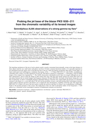


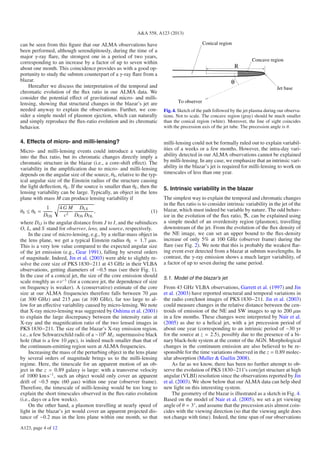


This document summarizes ALMA observations of the blazar PKS 1830-211 taken over multiple epochs in 2012. The blazar is lensed by a foreground galaxy, producing two resolved images (NE and SW) separated by 1". The observations were taken at frequencies corresponding to 350-1050 GHz in the blazar rest frame. Analysis of the flux ratio between the two images over time and frequency revealed a remarkable frequency-dependent behavior, implying a "chromatic structure" in the blazar jet. This is interpreted as evidence for a "core-shift effect" caused by plasmon ejection very near the base of the jet. The observations provide a unique probe of activity in the region where plasma acceleration occurs in blazar


