This study examined turbulence statistics over patchy vegetation at the Sevilleta National Wildlife Refuge to test the applicability of Monin-Obukhov similarity theory (MOST) over heterogeneous terrain. Measurements showed that the standard deviations and skewness of temperature followed MOST scaling, but the standard deviation of humidity was 28% larger, violating an MOST assumption. The temperature-humidity covariance coincidentally followed the same scaling as temperature variance, likely because their correlation was usually less than 0.8. This suggests MOST may not fully apply to the Sevilleta's meter-scale heterogeneous surface.
This document discusses methods for calculating the standard error of the b-value parameter in the Gutenberg-Richter magnitude-frequency relationship. It presents two key formulas:
1) For large samples where b can be treated as constant over time, the standard error of b is given by σ(b) = 2.30b2/√n, where n is the sample size and σ2(M) is the sample variance of magnitudes.
2) When b varies slowly over time, its standard error has two components - the time-averaged variance of b at different times, plus the variance of the mean b averaged over the entire time period.
The document also provides tables to determine confidence intervals for
This document proposes a modification to the Gutenberg-Richter law to describe the cumulative distribution of earthquake magnitudes using concepts from nonextensive statistical mechanics. It introduces a new "q-stretched exponential" form for the modified Gutenberg-Richter law and fits this form to seismic data from California and Iran. The empirical data fits extremely well with the proposed modification over the entire range of magnitudes. Nonextensive statistical mechanics is applied to derive a q-exponential distribution for the surface size of fragments produced during earthquakes. A new hypothetical relationship is also proposed between the surface size of fragments and the released energy.
This document discusses the distribution of slip along earthquake faults based on analyses of five major earthquake slip models. It finds that the distribution follows a piecewise Gutenberg-Richter law, with different b-values above and below a transition point. For smaller slips, b is near 1, while for larger slips b is greater than 1. It analyzes the slip distributions using rank-ordering analysis to overcome data limitations. This verifies the existence of power laws with different scaling constants in the two slip regimes identified.
This document discusses the statistical distributions of earthquake recurrence times and introduces a technique to analyze sequences of microearthquakes (microrepeaters). It specifically:
1) Discusses commonly used distributions like Weibull and log-normal to model recurrence times and introduces a rescaling technique to combine multiple microrepeater sequences to establish larger data sets.
2) Applies this technique to analyze recurrence times of microrepeater sequences from California and Japan.
3) Finds that when sequences are sufficiently stationary, the recurrence times can be well fitted by Weibull or log-normal distributions, demonstrating these distributions may also apply to characteristic earthquakes on major faults.
1) The document discusses the maximum likelihood estimator of b-value for mainshocks versus all events.
2) It shows that mainshocks do not entirely satisfy the Gutenberg-Richter law since their magnitude distribution depends on factors other than b-value alone.
3) Analyzing earthquake data from southern California, it demonstrates that the commonly used maximum likelihood estimator produces a statistically insignificant difference between b-values for mainshocks and all events when a more appropriate estimator is used that accounts for the non-exponential distribution of mainshock magnitudes.
This document provides instructions for analyzing the distribution of earthquakes based on magnitude, time, and location with a focus on clustering characteristics. It discusses Gutenberg-Richter's law which describes the relationship between earthquake magnitude and frequency. It also examines methods for calculating the b-value coefficient and considers the effects of aftershocks on magnitude distributions. The document proposes a model relating the magnitude distributions of main shocks, aftershocks, and all earthquakes based on b-values and the degree of aftershock activity.
This document summarizes methods for estimating the b-value parameter in the Gutenberg-Richter frequency-magnitude relationship for earthquakes. It reviews past estimation procedures and proposes a new method to estimate a slowly varying b-value over time using a moving time window. The method is applied to a dataset of California earthquakes between 1962-1981, finding no substantial variation in b-value.
1) The document examines the frequency-magnitude relationship for small earthquakes recorded at a borehole seismograph station in the Newport-Inglewood fault zone.
2) It finds a clear departure from the expected linear relationship for magnitudes below 3, with frequencies of M=0.5 earthquakes almost 10 times lower than expected.
3) This provides evidence that the frequency-magnitude relationship departs from self-similarity below about magnitude 3, coinciding with the observed departure of corner frequency from self-similarity. This supports the interpretation that the upper limit of large earthquake spectra (fmax) is related to fault zone size.
1) The paper investigates whether quantum variations around geodesics could circumvent caustics that occur in certain space-times.
2) An action is developed that yields both the field equations and geodesic condition. Quantizing this action provides a way to determine the extent of the wave packet around the classical path.
3) It is shown that replacing plane wave solutions with wave packets in the path integral still yields acceptable results. Determining if the distribution matches expectation values and variances is key to establishing geodesic completeness with quantum variations.
The document presents an experimental method to determine the effective mass of an oscillating spring. Measurements are made of the oscillation period T(n) of partial springs formed by hanging only n coils of a total N coil spring. A simple model relates T(n) to the effective mass and force constant of the partial spring. Testing various springs, the method provides values of the effective mass fraction f that are consistent with theoretical predictions for soft springs.
Mechanical wave descriptions for planets and asteroid fields: kinematic model...Premier Publishers
Models with wave dynamics and oscillations in the solar system are presented. A solitonial solution (Korteweg-de Vries), for a density field, is related to the formations of planets. A new nonlinear equation for a solitonial, will be derived, and denoted ‘J-T equation’. The linearized version has solutions, which are small vibrations with eigen frequency proportional to the parameters describing the solitonial wave, around a constant level, which is 2/3 of the maximum solitonial density. The location and orbital motion of Mercury and Venus are compared with wave dynamics. The tidal effect for Earth is analysed in terms of dynamics. Related phenomena for other planetary objects are discussed in conjunction with assuming a Roche limit.
1) The document summarizes the 100-year history of gravitational wave detection, from Einstein's theory of general relativity predicting their existence to the recent direct detection by the LIGO experiment.
2) It describes how LIGO uses laser interferometry to extremely sensitively measure tiny distortions in spacetime caused by passing gravitational waves.
3) The first detected gravitational waves in 2015 matched predictions for the inspiral and merger of two black holes, with the signal analyzed to determine properties of the black holes such as their masses.
Phase transition and the Casimir effect are studied in the complex scalar field with one spatial dimension to be compactified. It is shown that the phase transition is of the second order and the Casimir effect behaves quite differently
depending on whether it’s under periodic or anti-periodic boundary conditions
This document presents a non-extensive model for the frequency-magnitude distribution of earthquakes based on Tsallis entropy. The model assumes fragments between fault planes play an active role in triggering earthquakes. By applying maximum entropy principle with Tsallis entropy, the model derives an explicit function relating earthquake energy distribution to fragment size distribution. The function describes earthquake energy distributions over a wide range of energies. Analysis of earthquake data from southern Spain shows the model fits the data better than traditional Boltzmann statistics-based models, particularly for smaller magnitudes where other models fail.
This document presents the basic flow equations, including the Navier-Stokes equation and Euler's equations for frictionless flow. It also introduces several dimensionless numbers that are used to characterize different types of fluid flow and heat and mass transfer, such as the Reynolds number, Prandtl number, Schmidt number, and more. These equations and numbers provide a theoretical framework for analyzing fluid flow, while practical applications require further assumptions and simplifications.
This document proposes a new distribution model for earthquake magnitudes and intensities that addresses limitations of the traditional Gutenberg-Richter distribution model. Specifically, it introduces the generalized exponential distribution, which allows for an upper bound on magnitudes. The distribution is determined by analyzing both the overall distribution of magnitudes/intensities as well as the distribution of annual maximum values. An example is provided analyzing the intensity data of earthquakes in Zagreb over a 100-year period, finding that the generalized exponential distribution provides a good fit to the data.
Pratik Tarafdar is investigating the application of analogue gravity techniques to model primordial black hole accretion. He plans to apply these techniques used to model astrophysical black hole accretion to primordial black holes. This will help understand primordial black hole accretion phenomena from the perspective of analogue gravity. He has focused on calculating the analogue surface gravity and has obtained expressions for it in both adiabatic and isothermal cases for different accretion disk models. Future work will extend this to model radiation accretion onto primordial black holes and study effects of fluid dispersion on the analogue Hawking temperature.
- The document derives the second order Friedmann equations from the quantum corrected Raychaudhuri equation (QRE), which includes quantum corrections terms.
- One correction term can be interpreted as dark energy/cosmological constant with the observed density value, providing an explanation for the coincidence problem.
- The other correction term can be interpreted as a radiation term in the early universe that prevents the formation of a big bang singularity and predicts an infinite age for the universe by avoiding a divergence in the Hubble parameter or its derivative at any finite time in the past.
In this note, we derive (to third order in derivatives of the fluid velocity) a 2+1
dimensional theory of fluid dynamics that governs the evolution of generic long-
wavelength perturbations of a black brane or large black hole in four-dimensional
gravity with negative cosmological constant, applying a systematic procedure de-
veloped recently by Bhattacharyya, Hubeny, Minwalla, and Rangamani. In the
regime of validity of the fluid-dynamical description, the black-brane evolution
will generically correspond to a turbulent flow. Turbulence in 2+1 dimensions
has been well studied analytically, numerically, experimentally, and observation-
ally as it provides a first approximation to the large scale dynamics of planetary
atmospheres. These studies reveal dramatic differences between fluid flows in
2+1 and 3+1 dimensions, suggesting that the dynamics of perturbed four and
five dimensional large AdS black holes may be qualitatively different. However,
further investigation is required to understand whether these qualitative differ-
ences exist in the regime of fluid dynamics relevant to black hole dynamics.
1) The document proposes a theory of statistical geometrodynamics derived from novel statistical postulates about fundamental constituents of spacetime called "geomets".
2) Key results include deriving the Einstein field equations as a first law of geometrodynamics, and relating the Ricci curvature tensor to the entropy of a holographic surface bounding spacetime via a second law.
3) A third law and zeroeth law of geometrodynamics are also proposed, relating the mean curvature of the holographic surface to bit saturation in the bulk and on the surface.
Why Does the Atmosphere Rotate? Trajectory of a desorbed moleculeJames Smith
As a step toward understanding why the Earth's atmosphere "rotates" with the Earth, we use using Geometric (Clifford) Algebra to investigate the trajectory of a single molecule that desorbs vertically upward from the Equator, then falls back to Earth without colliding with any other molecules. Sample calculations are presented for a molecule whose vertical velocity is equal to the surface velocity of the Earth at the Equator (463 m/s) and for one with a vertical velocity three times as high. The latter velocity is sufficient for the molecule to reach the Kármán Line (100,000 m). We find that both molecules fall to Earth behind the point from which they desorbed: by 0.25 degrees of latitude for the higher vertical velocity, but by only 0.001 degrees for the lower.
Within the framework of the general theory of relativity (GR) the modeling of the central symmetrical
gravitational field is considered. The mapping of the geodesic motion of the Lemetr and Tolman basis on
their motion in the Minkowski space on the world lines is determined. The expression for the field intensity
and energy where these bases move is obtained. The advantage coordinate system is found, the coordinates
and the time of the system coincide with the Galilean coordinates and the time in the Minkowski space.
1. The document describes the VIPer22A, a low power offline SMPS primary switcher integrated circuit that combines a current mode PWM controller with a high voltage power MOSFET.
2. The VIPer22A has a wide input voltage range of 85-265V, output power capabilities of 7-20W, and a fixed switching frequency of 60kHz.
3. It features current mode control, undervoltage lockout, overtemperature protection, and can accommodate supply voltages from 9-38V on its VDD pin.
This document provides an overview of low voltage power MOSFET technologies, including trench MOSFETs, NexFETs, radiation hardened MOSFETs, and low voltage super-junction MOSFETs. It discusses the history and developments of trench MOSFET technology, advantages of the trench structure over VDMOS, and versions from Gen I-IV. NexFET technology is introduced as an improvement over trench MOSFETs by reducing parasitic capacitances. Radiation hardened MOSFETs are discussed in terms of failure mechanisms from radiation and hardening techniques. Finally, low voltage super-junction MOSFETs and the nextPower device are presented as an approach to achieve low RDS(on) at
(1) MOSFETs are field-effect transistors that use an electric field to control the conductivity of a channel. They have three terminals - the source, drain, and gate. (2) Depletion-type MOSFETs have a pre-existing channel between the source and drain, while enhancement-type MOSFETs require a positive gate voltage to induce a channel. (3) The key advantages of MOSFETs are that they are simpler to fabricate than bipolar junction transistors and take up less space on integrated circuits.
A MOSFET is a semiconductor device that can amplify or switch electronic signals. It has three terminals - drain, source, and gate. Depending on whether the semiconductor material between the drain and source is n-type or p-type, a MOSFET can be an n-channel or p-channel type. Applying a positive voltage to the gate of an n-channel MOSFET or a negative voltage to the gate of a p-channel MOSFET allows current to flow between the drain and source. MOSFETs are commonly used as switches in digital circuits like processors and as amplifiers in analog circuits. They are also used in memory devices, power supplies, and other electronic applications.
The MOSFET is an important element in embedded system design which is used to control the loads as per the requirement. The MOSFET is a high voltage controlling device provides some key features for circuit designers in terms of their overall performance.
Power Electronics and Switch Mode Power SupplyLiving Online
Power electronic circuits have revolutionised almost every device that we use today from PC's to TV's, microwave ovens and heavy industrial drives.
Switch Mode Power Supplies (SMPS) have thus become an important part of equipment design in all types of industrial equipment and an understanding of the different types and designs has become essential for reliable operation of complex equipment.
This workshop gives you a fundamental understanding of the basic components that form a SMPS design. You will understand how the selection of components affects the different performance parameters and operation of the SMPS. Typical practical applications of the SMPSs in industry will be discussed.
The concluding section of the workshop gives you the fundamental tools in troubleshooting SMPS designs confidently and effectively.
Even though the focus of the workshop is on the direct application of this technology, you will also gain a thorough understanding of the problems that can be introduced by SMPSs such as harmonics, electrostatic discharge and EMC/EMI problems.
WHO SHOULD ATTEND?
Anyone associated with the use of power electronics and switch mode power supply design techniques in the industrial or automation environment. The workshop will also benefit those working in system design as well as site commissioning, maintenance and troubleshooting.
Typical personnel who would benefit are:
Application engineers
Component suppliers
Electrical and electronic maintenance
Instrument for control engineers
Product designers
Product managers
Sales engineers
Service technicians
Supervisors
Technicians
MORE INFORMATION: http://www.idc-online.com/content/power-electronics-and-switch-mode-power-supply-38
A MOSFET (Metal Oxide Semiconductor Field Effect Transistor) is a semiconductor device that is commonly used in power electronics. It works by modulating charge concentration between a gate electrode, which is insulated from other device regions by an oxide layer, and a body region. Depending on whether it is an n-channel or p-channel MOSFET, the source and drain regions have either n+ or p+ doping while the body has the opposite doping. Applying a voltage to the gate can turn the channel between source and drain on or off to allow or prevent current flow. MOSFETs can be made with silicon on insulator or other semiconductor materials.
This document provides an introduction to transistors and MOSFETs. It begins by describing the invention of the transistor in 1947 and defining what a transistor is. It then discusses the main types of transistors - BJT and FET, including MOSFET and JFET. The rest of the document focuses on MOSFETs, explaining what they are, their terminals and symbols, types of MOSFETs like n-MOSFET and p-MOSFET, and how MOSFETs work and are fabricated through processes like photolithography, etching, diffusion, and oxidation. It includes diagrams of MOSFET structure and operation. In the end it briefly discusses CMOS fabrication process flow.
The document discusses different types of field effect transistors (FETs), including junction FETs (JFETs), metal-oxide-semiconductor FETs (MOSFETs), and metal-semiconductor FETs (MESFETs). It focuses on the structure and operation of n-channel and p-channel MOSFETs, describing how a positive or negative gate voltage is used to create a conducting channel. Scaling challenges for MOSFETs are also discussed, along with new materials needed like high-k dielectrics and metal gates, and approaches like silicon-on-insulator (SOI) technology.
This document discusses the basic principles of seismic waves. It introduces longitudinal (P) waves and shear (S) waves, and derives the one-dimensional wave equation. It discusses wave phenomena like reflection, transmission, and refraction based on Snell's law at boundaries between layers. It also discusses the different arrivals of direct, reflected, and refracted/head waves that can be measured at the surface for seismic exploration purposes.
This document summarizes an upcoming presentation on using computational modeling and experimental testing to better understand atmospheric entry of spacecraft. It discusses how different facilities can simulate some but not all entry conditions, and how multidisciplinary modeling is needed due to the complex coupled physics involved. Experimental testing in plasma wind tunnels can characterize the high-temperature reacting flow environment, while computational modeling requires approaches that span continuum to rarefied regimes to fully capture the multi-scale physics. Improving predictive capabilities will help design future planetary missions.
This document compares the statistical properties of solar flares and earthquakes by analyzing event energy distributions, time series, and interevent times from solar flare and earthquake catalogs. It finds that the two phenomena exhibit different scaling statistics, and the same phenomenon observed in different periods or locations cannot be uniformly scaled to a single distribution. This suggests an apparent complexity in impulsive energy release processes that does not follow a common behavior attributable to a universal physical mechanism.
This document summarizes a study that examines heat and mass transfer over a vertical plate in a porous medium with Soret and Dufour effects, a convective surface boundary condition, chemical reaction, and magnetic field. The governing equations for the fluid flow, heat transfer, and mass transfer are presented. Similarity solutions are used to transform the governing partial differential equations into ordinary differential equations, which are then solved numerically. The results are presented graphically to show the influence of various parameters on velocity, temperature, concentration, skin friction, Nusselt number, and Sherwood number.
International Journal of Mathematics and Statistics Invention (IJMSI) is an international journal intended for professionals and researchers in all fields of computer science and electronics. IJMSI publishes research articles and reviews within the whole field Mathematics and Statistics, new teaching methods, assessment, validation and the impact of new technologies and it will continue to provide information on the latest trends and developments in this ever-expanding subject. The publications of papers are selected through double peer reviewed to ensure originality, relevance, and readability. The articles published in our journal can be accessed online.
Earth-like lithospheric thickness and heat flow on Venus consistent with acti...Sérgio Sacani
Venus is Earth’s twin in size and radiogenic heat budget, yet it remains
unclear how Venus loses its heat absent plate tectonics. Most Venusian
stagnant-lid models predict a thick lithosphere with heat fow about half
that of Earth’s mobile-lid regime. Here we estimate elastic lithospheric
thickness at 75 locations on Venus using topographic fexure at 65 coronae—
quasi-circular volcano-tectonic features—determined from Magellan
altimetry data. We fnd an average thickness at coronae of 11 ± 7 km. This
implies an average heat fow of 101 ± 88 mW m−2, higher than Earth’ s
average but similar to terrestrial values in actively extending areas. For
some locations, such as the Parga Chasma rift zone, we estimate heat fow
exceeding 75 mW m−2. Combined with a low-resolution map of global elastic
thickness, this suggests that coronae typically form on thin lithosphere,
instead of locally thinning the lithosphere via plume heating, and that most
regions of low elastic thickness are best explained by high heat fow rather
than crustal compensation. Our analysis identifes likely areas of active
extension and suggests that Venus has Earth-like lithospheric thickness
and global heat fow ranges. Together with the planet’s geologic history,
our fndings support a squishy-lid convective regime that relies on plumes,
intrusive magmatism and delamination to increase heat fow.
Nonlinear Asymmetric Kelvin-Helmholtz Instability Of Cylindrical Flow With Ma...ijtsrd
The nonlinear asymmetric Kelvin-Helmholtz stability of the cylindrical interface between the vapor and liquid phases of a °uid is studied when the phases are enclosed between two cylindri- cal surfaces coaxial with the interface, and when there is mass and heat transfer across the inter- face. The method of multiple time expansion is used for the investigation. The evolution of am- plitude is shown to be governed by a nonlinear ¯rst order di®erential equation. The stability cri- terion is discussed, and the region of stability is displayed graphically. Also investigated in this paper is the viscous linear potential °ow. DOO-SUNG LEE"Nonlinear Asymmetric Kelvin-Helmholtz Instability Of Cylindrical Flow With Mass And Heat Transfer And The Viscous Linear Analysis" Published in International Journal of Trend in Scientific Research and Development (ijtsrd), ISSN: 2456-6470, Volume-2 | Issue-5 , August 2018, URL: http://www.ijtsrd.com/papers/ijtsrd17030.pdf http://www.ijtsrd.com/mathemetics/applied-mathematics/17030/nonlinear-asymmetric-kelvin-helmholtz-instability-of-cylindrical-flow-with-mass-and-heat-transfer-and-the-viscous-linear-analysis/doo-sung-lee
Artigo que descreve o trabalho feito com o Chandra nos aglomerados de galáxias de Perseus e Virgo sobre a descoberta de uma turbulência cósmica que impede a formação de novas estrelas.
This document discusses equations related to heat transfer through pipes and the temperature gradient that results from fluid flow. It then speculates that quantum mechanical equations like the Fermi-Dirac distribution and theories of relativity may help explain the relationship between temperature and the movement of water particles through pipes. The document proposes that the velocity of water particles must be connected to temperature, that velocity is infinite, and that the movement of an inertial system through a vacuum must be related to the movement of the system.
Magneto convective flowand heat transfer of two immiscible fluids between ver...eSAT Publishing House
IJRET : International Journal of Research in Engineering and Technology is an international peer reviewed, online journal published by eSAT Publishing House for the enhancement of research in various disciplines of Engineering and Technology. The aim and scope of the journal is to provide an academic medium and an important reference for the advancement and dissemination of research results that support high-level learning, teaching and research in the fields of Engineering and Technology. We bring together Scientists, Academician, Field Engineers, Scholars and Students of related fields of Engineering and Technology
This document presents a numerical solution for unsteady heat and mass transfer flow past an infinite vertical plate with variable thermal conductivity, taking into account Dufour number and heat source effects. The governing equations are non-linear and coupled, and were solved numerically using an implicit finite difference scheme. Various parameters, including Dufour number and heat source, were found to influence the velocity, temperature, and concentration profiles. Skin friction, Nusselt number, and Sherwood number were also calculated.
Nanofluid Flow past an Unsteady Permeable Shrinking Sheet with Heat Source or...IJERA Editor
The consideration of nanofluids has been paid a good attention on the forced convection; the analysis focusing
nanofluids in porous media are limited in literature. Thus, the use of nanofluids in porous media would be very
much helpful in heat and mass transfer enhancement. In this paper, the influence of variable suction, Newtonian
heating and heat source or sink heat and mass transfer over a permeable shrinking sheet embedded in a porous
medium filled with a nanofluid is discussed in detail. The solutions of the nonlinear equations governing the
velocɨty, temperature and concentration profiles are solved numerically using Runge-Kutta Gill procedure
together with shooting method and graphical results for the resulting parameters are displayed and discussed.
The influence of the physical parameters on skin-friction coefficient, local Nusselt number and local Sherwood
number are shown in a tabulated form.
This document presents a sensitivity analysis of the combination evapotranspiration equation, which estimates potential evapotranspiration (PET). Sensitivity equations were derived by differentiating the combination equation with respect to each variable. Applying two years of daily data from Iowa, the sensitivity coefficients showed that computed PET is most sensitive to net radiation. During midyear, a 50-90% change in radiation results in the same percentage change in PET, while a change in vapor pressure deficit or wind only changes PET by 20-30%. In spring and fall, aerodynamic variables like wind have a larger effect on PET values. Overall, the analysis provides insight into the relative impact of each variable in the evapotranspiration equation.
This chapter discusses heat transfer through porous media. It begins by presenting the basic energy equations for a simple case where the solid and fluid phases are in local thermal equilibrium and heat conduction occurs in parallel through the phases. It then discusses extensions to more complex situations, including how the overall thermal conductivity depends on the geometry and properties of the solid and fluid, and the effects of pressure changes and viscous dissipation. The overall thermal conductivity can be estimated using weighted arithmetic, harmonic, or geometric means of the solid and fluid conductivities. More complex models have also been developed to account for factors like anisotropy, Knudsen effects, and material microstructure.
EXPERIMENTAL AND NUMERICAL INVESTIGATIONS OF A TURBULENT BOUNDARY LAYER UNDER...Barhm Mohamad
In this article we present an experimental and numerical study of the behavior of the boundary layer type viscous flow in the presence of the thermal effect. The flow was held in a three-dimensional field with a uniform infinite velocity in the case of an adiabatic wall with heat input. The presented experimental work was performed in the Thermal Laboratory (LET) of the Prime Institute of Poitiers (France). It describes the analysis of a turbulent boundary layer created in a wind tunnel on the surface of a flat plate covered with epoxy resin. An HP 6012A power supply system was used to provide circulating heat flux to heat the flat plate to 80°C by the Joule effect. The numerical result shows a clear difference in the evolution of the thermal boundary layer between the three temperatures of the wall.
Derivation and solution of the heat equation in 1-DIJESM JOURNAL
Heat flows in the direction of decreasing temperature, that is, from hot to cool. In this paper we derive the heat equation and consider the flow of heat along a metal rod. The rod allows us to consider the temperature, u(x,t), as one dimensional in x but changing in time, t.
Numerical Analysis of heat transfer in a channel Wit in clined bafflesinventy
Research Inventy : International Journal of Engineering and Science is published by the group of young academic and industrial researchers with 12 Issues per year. It is an online as well as print version open access journal that provides rapid publication (monthly) of articles in all areas of the subject such as: civil, mechanical, chemical, electronic and computer engineering as well as production and information technology. The Journal welcomes the submission of manuscripts that meet the general criteria of significance and scientific excellence. Papers will be published by rapid process within 20 days after acceptance and peer review process takes only 7 days. All articles published in Research Inventy will be peer-reviewed.
FREE CONVECTION HEAT TRANSFER OF NANOFLUIDS FROM A HORIZONTAL PLATE EMBEDDED ...AEIJjournal2
In this paper the natural convection heat transfer from a horizontal plate embedded in a porous medium
saturated with a nanofluid is numerically analyzed. By a similarity approach the partial differential
equations are reduced to a set of two ordinary differential equations. In order to evaluate the influence of
nanoparticles on the heat transfer, Ag and Cuo as the nanoparticles were selected. Results show that heat
transfer rate (Nur) is a decreasing function of volume fraction of nanoparticles.
The Future of Independent Filmmaking Trends and Job OpportunitiesLetsFAME
The landscape of independent filmmaking is evolving at an unprecedented pace. Technological advancements, changing consumer preferences, and new distribution models are reshaping the industry, creating new opportunities and challenges for filmmakers and film industry jobs. This article explores the future of independent filmmaking, highlighting key trends and emerging job opportunities.
The Evolution of the Leonardo DiCaprio Haircut: A Journey Through Style and C...greendigital
Leonardo DiCaprio, a name synonymous with Hollywood stardom and acting excellence. has captivated audiences for decades with his talent and charisma. But, the Leonardo DiCaprio haircut is one aspect of his public persona that has garnered attention. From his early days as a teenage heartthrob to his current status as a seasoned actor and environmental activist. DiCaprio's hairstyles have evolved. reflecting both his personal growth and the changing trends in fashion. This article delves into the many phases of the Leonardo DiCaprio haircut. exploring its significance and impact on pop culture.
Odia New Web Series at your fingerprint.mikedanoffice
Stay ahead of the curve with the latest in Odia entertainment! Our Odia new web series promise an exciting blend of fresh narratives, talented performances, and engaging plots. Immerse yourself in the evolving world of Odia storytelling with our curated selection of cutting-edge web content. for more visit: https://aaonxt.com/series
Leonardo DiCaprio House: A Journey Through His Extravagant Real Estate Portfoliogreendigital
Introduction
Leonardo DiCaprio, A name synonymous with Hollywood excellence. is not only known for his stellar acting career but also for his impressive real estate investments. The "Leonardo DiCaprio house" is a topic that piques the interest of many. as the Oscar-winning actor has amassed a diverse portfolio of luxurious properties. DiCaprio's homes reflect his varied tastes and commitment to sustainability. from retreats to historic mansions. This article will delve into the fascinating world of Leonardo DiCaprio's real estate. Exploring the details of his most notable residences. and the unique aspects that make them stand out.
Follow us on: Pinterest
Leonardo DiCaprio House: Malibu Beachfront Retreat
A Prime Location
His Malibu beachfront house is one of the most famous properties in Leonardo DiCaprio's real estate portfolio. Situated in the exclusive Carbon Beach. also known as "Billionaire's Beach," this property boasts stunning ocean views and private beach access. The "Leonardo DiCaprio house" in Malibu is a testament to the actor's love for the sea and his penchant for luxurious living.
Architectural Highlights
The Malibu house features a modern design with clean lines, large windows. and open spaces blending indoor and outdoor living. The expansive deck and patio areas provide ample space for entertaining guests or enjoying a quiet sunset. The house has state-of-the-art amenities. including a gourmet kitchen, a home theatre, and many guest suites.
Sustainable Features
Leonardo DiCaprio is a well-known environmental activist. whose Malibu house reflects his commitment to sustainability. The property incorporates solar panels, energy-efficient appliances, and sustainable building materials. The landscaping around the house is also designed to be water-efficient. featuring drought-resistant plants and intelligent irrigation systems.
Leonardo DiCaprio House: Hollywood Hills Hideaway
Privacy and Seclusion
Another remarkable property in Leonardo DiCaprio's collection is his Hollywood Hills house. This secluded retreat offers privacy and tranquility. making it an ideal escape from the hustle and bustle of Los Angeles. The "Leonardo DiCaprio house" in Hollywood Hills nestled among lush greenery. and offers panoramic views of the city and surrounding landscapes.
Design and Amenities
The Hollywood Hills house is a mid-century modern gem characterized by its sleek design and floor-to-ceiling windows. The open-concept living space is perfect for entertaining. while the cozy bedrooms provide a comfortable retreat. The property also features a swimming pool, and outdoor dining area. and a spacious deck that overlooks the cityscape.
Environmental Initiatives
The Hollywood Hills house incorporates several green features that are in line with DiCaprio's environmental values. The home has solar panels, energy-efficient lighting, and a rainwater harvesting system. Additionally, the landscaping designed to support local wildlife and promote
Sara Saffari: Turning Underweight into Fitness Success at 23get joys
Uncover the remarkable journey of Sara Saffari, whose transformation from underweight struggles to being recognized as a fitness icon at 23 underscores the importance of perseverance, discipline, and embracing a healthy lifestyle.
From Teacher to OnlyFans: Brianna Coppage's Story at 28get joys
At 28, Brianna Coppage left her teaching career to become an OnlyFans content creator. This bold move into digital entrepreneurship allowed her to harness her creativity and build a new identity. Brianna's experience highlights the intersection of technology and personal branding in today's economy.
The Unbelievable Tale of Dwayne Johnson Kidnapping: A Riveting Sagagreendigital
Introduction
The notion of Dwayne Johnson kidnapping seems straight out of a Hollywood thriller. Dwayne "The Rock" Johnson, known for his larger-than-life persona, immense popularity. and action-packed filmography, is the last person anyone would envision being a victim of kidnapping. Yet, the bizarre and riveting tale of such an incident, filled with twists and turns. has captured the imagination of many. In this article, we delve into the intricate details of this astonishing event. exploring every aspect, from the dramatic rescue operation to the aftermath and the lessons learned.
Follow us on: Pinterest
The Origins of the Dwayne Johnson Kidnapping Saga
Dwayne Johnson: A Brief Background
Before discussing the specifics of the kidnapping. it is crucial to understand who Dwayne Johnson is and why his kidnapping would be so significant. Born May 2, 1972, Dwayne Douglas Johnson is an American actor, producer, businessman. and former professional wrestler. Known by his ring name, "The Rock," he gained fame in the World Wrestling Federation (WWF, now WWE) before transitioning to a successful career in Hollywood.
Johnson's filmography includes blockbuster hits such as "The Fast and the Furious" series, "Jumanji," "Moana," and "San Andreas." His charismatic personality, impressive physique. and action-star status have made him a beloved figure worldwide. Thus, the news of his kidnapping would send shockwaves across the globe.
Setting the Scene: The Day of the Kidnapping
The incident of Dwayne Johnson's kidnapping began on an ordinary day. Johnson was filming his latest high-octane action film set to break box office records. The location was a remote yet scenic area. chosen for its rugged terrain and breathtaking vistas. perfect for the film's climactic scenes.
But, beneath the veneer of normalcy, a sinister plot was unfolding. Unbeknownst to Johnson and his team, a group of criminals had planned his abduction. hoping to leverage his celebrity status for a hefty ransom. The stage was set for an event that would soon dominate worldwide headlines and social media feeds.
The Abduction: Unfolding the Dwayne Johnson Kidnapping
The Moment of Capture
On the day of the kidnapping, everything seemed to be proceeding as usual on set. Johnson and his co-stars and crew were engrossed in shooting a particularly demanding scene. As the day wore on, the production team took a short break. providing the kidnappers with the perfect opportunity to strike.
The abduction was executed with military precision. A group of masked men, armed and organized, infiltrated the set. They created chaos, taking advantage of the confusion to isolate Johnson. Johnson was outnumbered and caught off guard despite his formidable strength and fighting skills. The kidnappers overpowered him, bundled him into a waiting vehicle. and sped away, leaving everyone on set in a state of shock and disbelief.
The Immediate Aftermath
The immediate aftermath of the Dwayne Johnson kidnappin
Leonardo DiCaprio Super Bowl: Hollywood Meets America’s Favorite Gamegreendigital
Introduction
Leonardo DiCaprio is synonymous with Hollywood stardom and acclaimed performances. has a unique connection with one of America's most beloved sports events—the Super Bowl. The "Leonardo DiCaprio Super Bowl" phenomenon combines the worlds of cinema and sports. drawing attention from fans of both domains. This article delves into the multifaceted relationship between DiCaprio and the Super Bowl. exploring his appearances at the event, His involvement in Super Bowl advertisements. and his cultural impact that bridges the gap between these two massive entertainment industries.
Follow us on: Pinterest
Leonardo DiCaprio: The Hollywood Icon
Early Life and Career Beginnings
Leonardo Wilhelm DiCaprio was born in Los Angeles, California, on November 11, 1974. His journey to stardom began at a young age with roles in television commercials and educational programs. DiCaprio's breakthrough came with his portrayal of Luke Brower in the sitcom "Growing Pains" and later as Tobias Wolff in "This Boy's Life" (1993). where he starred alongside Robert De Niro.
Rise to Stardom
DiCaprio's career skyrocketed with his performance in "What's Eating Gilbert Grape" (1993). earning him his first Academy Award nomination. He continued to gain acclaim with roles in "Romeo + Juliet" (1996) and "Titanic" (1997). the latter of which cemented his status as a global superstar. Over the years, DiCaprio has showcased his versatility in films like "The Aviator" (2004). "Start" (2010), and "The Revenant" (2015), for which he finally won an Academy Award for Best Actor.
Environmental Activism
Beyond his film career, DiCaprio is also renowned for his environmental activism. He established the Leonardo DiCaprio Foundation in 1998, focusing on global conservation efforts. His commitment to ecological issues often intersects with his public appearances. including those related to the Super Bowl.
The Super Bowl: An American Institution
History and Significance
The Super Bowl is the National Football League (NFL) championship game. is one of the most-watched sporting events in the world. First played in 1967, the Super Bowl has evolved into a cultural phenomenon. featuring high-profile halftime shows, memorable advertisements, and significant media coverage. The event attracts a diverse audience, from avid sports fans to casual viewers. making it a prime platform for celebrities to appear.
Entertainment and Advertisements
The Super Bowl is not only about football but also about entertainment. The halftime show features performances by some of the biggest names in the music industry. while the commercials are often as anticipated as the game itself. Companies invest millions in Super Bowl ads. creating iconic and sometimes controversial commercials that capture public attention.
Leonardo DiCaprio's Super Bowl Appearances
A Celebrity Among the Fans
Leonardo DiCaprio's presence at the Super Bowl has noted several times. As a high-profile celebrity. DiCaprio attracts
Abraham Laboriel Records ‘The Bass Walk’ at Evergreen Stage
15832945
1. STATISTICS OF SURFACE-LAYER TURBULENCE OVER TERRAIN
WITH METRE-SCALE HETEROGENEITY
EDGAR L ANDREAS1 , REGINALD J. HILL2 , JAMES R. GOSZ3 ,
DOUGLAS I. MOORE3 , WILLIAM D. OTTO2 and ACHANTA D. SARMA4
1
U.S. Army Cold Regions Research and Engineering Laboratory, 72 Lyme Road, Hanover, New
Hampshire 03755-1290, U.S.A.
2
National Oceanic and Atmospheric Administration, Environmental Technology Laboratory, 325
Broadway, Boulder, Colorado 80303-3328, U.S.A.
3
Biology Department, University of New Mexico, Albuquerque, New Mexico 87131, U.S.A.
4
R. & T. Unit for Navigational Electronics, Osmania University, Hyderabad – 500007, India
(Received in final form 23 June, 1997)
Abstract. The Sevilleta National Wildlife Refuge has patchy vegetation in sandy soil. During midday
and at night, the surface sources and sinks for heat and moisture may thus be different. Although
the Sevilleta is broad and level, its metre-scale heterogeneity could therefore violate an assumption
on which Monin-Obukhov similarity theory (MOST) relies. To test the applicability of MOST in
such a setting, we measured the standard deviations of vertical (w ) and longitudinal velocity (u ),
temperature (t ), and humidity (q ), the temperature-humidity covariance (tq ), and the temperature
skewness (St ). Dividing the former five quantities by the appropriate flux scales (u , t , and q )
j j j j j j
yielded the nondimensional statistics w =u , u =u , t = t , q = q , and tq=t q . w =u , t = t ,
and St have magnitudes and variations with stability similar to those reported in the literature and,
thus, seem to obey MOST. Though u =u is often presumed not to obey MOST, our u =u data also
j j
agree with MOST scaling arguments. While q = q has the same dependence on stability as t = t , j j
its magnitude is 28% larger. When we ignore tq=t q values measured during sunrise and sunset
transitions – when MOST is not expected to apply – this statistic has essentially the same magnitude
and stability dependence as t =t 2 . In a flow that truly obeys MOST, t =t 2 , q =q 2 , and
tq=t q should all have the same functional form. That q =q 2 differs from the other two suggests
that the Sevilleta has an interesting surface not compatible with MOST. The sources of humidity
reflect the patchiness while, despite the patchiness, the sources of heat seem uniformly distributed.
Key words: Bowen ratio, Heterogeneous terrain, Monin–Obukhov similarity, Skewness of temper-
ature, Sonic anemometer/thermometer, Statistics of turbulence
1. Introduction
Monin–Obukhov similarity theory (MOST) has been the most important develop-
ment in boundary-layer meteorology in the last 50 years. By unifying the inter-
pretation of diverse observations, it provided the theoretical foundation on which
boundary-layer meteorology has risen as a discipline.
Yet, despite the success of MOST in unifying theory and observations, disturb-
ing uncertainties persist in some of the universal functions that it predicts should
exist. Compare, for example, the recent summaries by Panofsky and Dutton (1984),
Sorbjan (1989), and Kaimal and Finnigan (1994). In light of this persistent uncer-
tainty, it is still important to report high-quality turbulence data that may help
Boundary-Layer Meteorology 86: 379–408, 1998.
c 1998 Kluwer Academic Publishers. Printed in the Netherlands.
2. 380 EDGAR L ANDREAS ET AL.
narrow the error bars on the Monin–Obukhov similarity functions and, indeed,
answer questions about MOST’s applicability.
Although MOST is founded on the assumption of horizontal homogeneity, it
really is the only conceptual framework we have for treating near-surface turbulence
in the atmospheric boundary layer. Consequently, much current research focuses
on extending MOST to heterogeneous surfaces (e.g., Beljaars and Holtslag, 1991;
Roth and Oke, 1993; Roth, 1993; Katul et al., 1995).
Here our objective is also to use MOST to investigate turbulence statistics over
a heterogeneous surface – but one that is heterogeneous only at scales from tens
of centimetres to several metres. At larger scales, our site is homogeneous. We did
our work at the Sevilleta National Wildlife Refuge, a semi-arid grassland between
Albuquerque and Socorro, New Mexico. The Sevilleta’s vegetation is patchy, with
bare ground between clumps of plants. It is easy to imagine that, during daytime,
the bare ground is a heat source in the late summer, and the plants are water vapour
sources. Because of this source heterogeneity, the statistics of temperature and
humidity and, especially, their covariance might not follow the same similarity
relations, as MOST predicts they should (Hill, 1989).
Our results, however, suggest that the surface heat sources are not as heteroge-
neous as the plant cover. The measured nondimensional temperature variance and
temperature skewness values follow Monin–Obukhov similarity functions similar
to those already reported in the literature. The nondimensional humidity variance,
on the other hand, follows a similarity relation that is 60% above the temperature
relation. But then the nondimensional temperature-humidity covariance coinciden-
tally follows practically the same similarity relation as does temperature variance.
This latter result is possible because the temperature-humidity correlation coeffi-
cient – even during stationary periods – typically has an absolute value of 0.8 or
less. We conclude that this behaviour of the temperature-humidity covariance is
evidence of how the Sevilleta’s metre-scale heterogeneity leads to violations of
MOST. In a flow that strictly obeys MOST, the correlation coefficient between any
two conservative scalars must be 1 (Hill, 1989).
2. Theoretical Background
Monin–Obukhov similarity theory predicts the following relationships (e.g., Wyn-
gaard, 1973; Sorbjan, 1989, p. 69 ff.; Hill, 1989):
w = (z=L);
u 33 (2.1)
t = (z=L);
jt j tt (2.2)
q
jqj = qq (z=L); (2.3)
3. STATISTICS OF SURFACE-LAYER TURBULENCE 381
tq = (z=L):
tq tq (2.4)
Here, w , t , and q are the standard deviations in vertical velocity, temperature,
and specific humidity, and tq is the temperature-humidity covariance, where t and
q are, respectively, the turbulent fluctuations in temperature and specific humidity,
and the overbar denotes a time average. u , t , and q are flux scales such that
u2 = uw, ut = wt, and uq = wq are, respectively, the kinematic
surface stress, temperature flux, and specific humidity flux. In addition, z is the
measurement height, and L is the Obukhov length,
L 1 = gkwt3v ;
Tv u (2.5)
where g is the acceleration of gravity, k (= 0.4) is the von K´ rm´ n constant,
a a
Tv = T (1 + 0:61Q) (2.6)
is a representative virtual temperature of the atmospheric surface layer (ASL), and
wtv = wt(1 + 0:61Q) + 0:61Twq (2.7)
is the virtual temperature flux. Also in (2.6) and (2.7), T and Q are representative
surface-layer values of air temperature and specific humidity.
In Equations (2.1)–(2.4), the crux of MOST is the functions; these are nondi-
mensional – presumably universal – functions of the stability parameter z=L.
Although MOST predicts that universal forms for should exist, the actual func-
tions must be found experimentally. MOST does, however, provide insights into
the functional forms of the s for very unstable and very stable stratification.
Because in very unstable or free-convection conditions, u loses its significance
as the appropriate velocity scale, it is common to define a free-convection velocity
scale (e.g., Hess, 1992)
=
!1 3
uf = zgwtv :
Tv (2.8)
This scale, in turn, lets us define new temperature and humidity scales,
=
!1 3
wt = Tv wt3
tf = u ;
f zgwtv (2.9)
=
!1 3
qf = wq = Tv wq
3
uf zgwtv : (2.10)
4. 382 EDGAR L ANDREAS ET AL.
Because u and, thus, t and q lose their significance gradually as the ASL
approaches free convection, we can recast Equations (2.8)–(2.10) for large as
uf = k 1=3 ( )1=3;
u (2.11)
tf = qf = k1=3( ) 1=3 :
t q (2.12)
The three scales uf , tf , and qf , with (2.11) and (2.12), lead immediately to the
well-known predictions for the asymptotic behaviours of 33 , tt , and qq in free
convection (e.g., Wyngaard, 1973; Sorbjan, 1989, p. 71 ff.),
33 ( ) = A3u ( )1=3; (2.13)
tt ( ) = Atu( ) 1=3 ; (2.14)
qq ( ) = Aqu( ) 1=3; (2.15)
where A3u , Atu , and Aqu are constants.
In very stable conditions, the turbulent eddies are small and often never interact
with the surface. Consequently, the height of the observation, z , has no significance.
This is z -less stratification (Wyngaard, 1973; Dias et al., 1995). MOST suggests that
the asymptotic behaviours of the functions in the limit of very stable stratification
(i.e., large ) are
33 ( ) = A3s; (2.16)
tt ( ) = Ats; (2.17)
qq ( ) = Aqs; (2.18)
where A3s , Ats , and Aqs are constants.
We also study the temperature skewness,
t3
St 3 ; (2.19)
t
where t3 is the third moment of temperature. Businger (1973) stated that it is not
possible to use MOST to predict the asymptotic behaviour of St , as has been done
for 33 , tt , and qq . He now, however, agrees that the following MOST arguments
are accurate (J. A. Businger, 1995, personal communication).
We can rewrite St as
t3 tf 3 jtj 3 :
St = t3 t
f t (2.20)
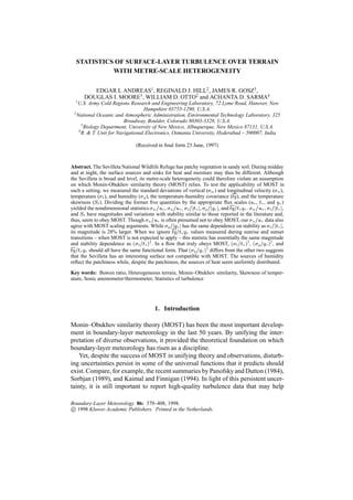
5. STATISTICS OF SURFACE-LAYER TURBULENCE 383
In the asymptotic limit of free convection (i.e., large ),
t3 = Bu;
t3
f
(2.21)
a constant. Thus, substituting (2.12), (2.14), and (2.21) in (2.20) yields
St = Bu[k( ) 1
][Atu3 ( )] = kBu=A3 ;
tu (2.22)
a constant. That is, in the free-convection limit, MOST predicts that St becomes a
constant.
In very stable conditions (i.e., for large ), on the other hand, MOST suggests
t3 = B ;
t3 s (2.23)
yet another constant. But we can also rewrite the skewness as
St = t3 j j :
t3 t 3 (2.24)
t
Thus, with (2.17) and (2.23), (2.24) becomes
St = Bs=A3 ;
ts (2.25)
which is again a constant. That is, in z -less stratification also, St approaches a
constant.
Monin and Yaglom (1971, p. 462) also give these two asymptotic predictions
for temperature skewness, but without proof. The same arguments also hold for
humidity skewness.
3. The Sevilleta
The Sevilleta National Wildlife Refuge is in the rift valley of the Rio Grande
River; our research site was in the area known as McKenzie Flats (34 210 5.1500 N,
106 410 9.4700 W). Although mountains rise 1000 m above the valley floor to the
east and to the far west, McKenzie Flats itself is a large (100 km2 ) grassland
area that is relatively level and fairly homogeneous at kilometre scales. Otto et al.
(1995) give other details of the site, including maps.
On a scale of tens of centimetres to several metres, however, the Sevilleta’s
vegetation is patchy (see Figure 1). Vegetation transect studies are done annually in
this area. These consist of 400-m-line-intercept measurements at 1 cm resolution
that yield percentages covered by bare ground, litter, and various plant species.
6. 384 EDGAR L ANDREAS ET AL.
Figure 1. Patchy vegetation characterizes the Sevilleta. The patchiness, however, is visible only in
the foreground here because the vegetation occludes the line-of-sight in the background. In the insert,
the scale is in centimetres.
7. STATISTICS OF SURFACE-LAYER TURBULENCE 385
In the late summer of 1991, vegetation covered 37.7% of the area; bare ground,
33.3%; and litter, 29.0%. The dominant plant species (see Figure 1) were black
grama (Bouteloua eripoda), with 18.0% coverage, and blue grama (Bouteloua
gracilis), with 8.8% coverage. These values also correspond closely to the leaf area
index because of the low stature of these plants.
During our experiment, plant pedestals, typically, were 5 cm above the surface,
leaves reached 30 cm, and seed stalks reached 60 cm. The spacing between clumps
of plants was on the order 20–30 cm. Turner et al. (1991) and Gosz (1993, 1995)
give additional details of the Sevilleta’s vegetation.
We collected the data described here on 4–16 August 1991. August is the rainy
season in New Mexico. The Sevilleta had, at least, light rain on 10 of the 13 days
of our experiment. Some storms yielded heavy rain, with one log entry showing 1
cm of rain in an hour. Dew was common in the morning. As a consequence, the
turbulent sensible and latent heat fluxes were, generally, of comparable magnitude.
4. The Data
4.1. DATA COLLECTION AND PROCESSING
A three-axis ‘Kaimal’ sonic anemometer/thermometer made by Applied Technolo-
gies, Inc. (ATI; Boulder, Colorado) was our primary turbulence instrument. This
was positioned at the top of a thin beam with the center of the w-anemometer path
4 m above the ground. A sampling height of 4 m is sufficient to allay concern over
the loss of high-frequncy response because of the path-averaging in this instrument
(Kaimal and Finnigan, 1994, p. 219). The ATI sonic provides digital values of the
three velocity components and temperature 10 times per second. We logged these
data through the communications port of a personal computer. Each three-axis
sonic run started on the hour and continued for 40.96 minutes. We made 69 such
runs.
After the experiment, we computed the turbulence statistics for each sonic run.
This analysis included routines to remove spikes and detrend the time series. We
also rotated the statistics into a coordinate frame in which the mean transverse and
vertical velocity components and the mean transverse turbulent stresses were all
zero. The statistics thus computed included run averages of uw , wt, u , t , L, w ,
u, t , and t3 , where u is the standard deviation in longitudinal velocity.
Fifty metres southeast of the three-axis sonic tower was our so-called eddy-
correlation tower that held turbulence instruments made by Campbell Scientific,
Inc. (Logan, Utah). Here, again 4 m above the ground, were a vertically oriented
single-axis sonic anemometer, a 76-m chromel-constantan thermocouple, and a
krypton hygrometer. A Campbell data logger sampled these instruments at 10 Hz
and automatically computed averages from the top of the hour to 40 minutes after
the hour; these eddy-correlation statistics, thus, coincided with those from the
8. 386 EDGAR L ANDREAS ET AL.
three-axis sonic. Statistics from these instruments included w , t , q , wt, wq , and
tq. We have 118 runs with these data. Using u from the three-axis sonic, we could
also compute t and q from these data. There are 30 of these coincident runs.
Midway between the sonic and eddy-correlation towers was a Campbell Bowen
ratio station. This measured the Bowen ratio, defined as
Bo = Lpwt = Lptq ;
c
wq
c (4.1)
v v
by measuring temperature and dew point at two heights. That is, the Bowen ratio
station approximated the Bowen ratio as
Bo = L p(Q2 T1 )) :
c (T
v 2 Q1
(4.2)
In (4.1) and (4.2), cp is the specific heat of air at constant pressure, and Lv is the
latent heat of vaporization of water. On this Bowen-ratio tower, matched 76-m-
diameter chromel-constantan thermocouples placed at heights of 0.87 and 2.83 m
measured the vertical temperature gradient. At the same two heights, air intakes
led to a single cooled-mirror dew-point hygrometer. At 2-minute intervals, a pump
and valve alternately sent air from one intake and then the other to the hygrometer.
The dew points at the two heights were thus measured. A second Campbell data
logger, again synchronized to sample for 40 minutes starting on the hour, collected
these temperature and dew-point data, calculated the vertical temperature (T2 T1)
and specific humidity (Q2 Q1 ) differences, and output 40-minute averages of
the Bowen ratio estimated according to (4.2). Although the Bowen ratio station
yielded other data, which we mention briefly later, here we primarily use these
Bowen ratios (in the Appendix).
Schotanus et al. (1983) and Kaimal and Gaynor (1991) explain that the tem-
perature measured by a sonic thermometer is not a true temperature; it contains
humidity information also. If ts is the instantaneous temperature measured by a
e
sonic thermometer,
tes = t(1 + 0:51q);
~ ~ (4.3)
where t and q are the instantaneous temperature and specific humidity in the sonic
~ ~
path. Notice, (4.3) is not very different from the virtual temperature, (2.6). Kaimal
and Gaynor demonstrate that the sonic temperature can, therefore, be used directly
for computing the Obukhov length [see (2.5)] without humidity corrections.
Since we also use the sonic temperature to compute t and t3 , we worry that
these might be biased by humidity. In the Appendix, however, we demonstrate
that, for the range of Bowen ratios we encountered, the statistics of interest here,
t=jt j and t3=t3 , can be computed directly from the sonic temperature without
corrections for humidity.
9. STATISTICS OF SURFACE-LAYER TURBULENCE 387
4.2. QUALITY CONTROL
The three-axis ATI sonic anemometer/thermometer and the fast-responding tem-
perature and humidity sensors on the eddy-correlation tower were fixed in place
to accept southerly winds coming up the Rio Grande Valley. Of course, the winds
were not always head-on to the ATI sonic. But because of the thoughtful design of
this instrument, it can measure the wind vector accurately even in flows that are not
head-on. Kaimal et al. (1990) show that this anemometer has no directional bias
for winds 45 from head-on. We, however, interpret their data as suggesting that
there is no bias for winds to almost 90 from head-on.
We graded our sonic runs on the basis of mean wind direction and the variability
in the direction. We label runs with an average wind direction within 90 of head-
on to the sonic and with small directional variability our ‘best’ data, and those with a
mean wind direction within 90 of head-on but with higher directional variability
‘questionable’ data. We reject runs with winds coming predominantly from the
backside of the sonic or with high directional variability. Figure 2 shows wind-
direction histograms for typical runs that we identified as ‘best’, ‘questionable’,
and ‘rejected’.
Of the 69 original runs, we judged 31 as ‘best’ and 11 as ‘questionable’ and
rejected 27 for use in our analysis. As will be seen later, most of the questionable
runs occurred in lighter winds and were therefore associated with moderately
unstable stratification.
5. Turbulence Statistics
5.1. DISPLACEMENT HEIGHT
Over surfaces with vegetation, it is often necessary to account for the displacement
height d in the scaling. Then in Equations (2.1)–(2.4), for example, the correct
height scale would not be the height above ground z but rather z d (e.g., Lloyd et
al., 1991; Roth, 1993; Roth and Oke, 1993). Typically, d is 60–70% of the height
h of the vegetation if the vegetation is dense (Stanhill, 1969; Monteith, 1980;
Wieringa, 1993). With the patchy vegetation of the Sevilleta, however, we suspect
that d will be a smaller percentage of h (Wieringa, 1993). Since d is interpreted as
the average height within a canopy where the momentum is absorbed (Raupach,
1992; Wieringa, 1993), h at the Sevilleta would be the height below which the
plants are most dense. That is, h should be roughly what we earlier called the leaf
height, 30 cm. Hence, d may have been as large as 20 cm during our experiment
but likely was smaller.
Since d is defined in the context of momentum exchange, we can investigate its
importance to us by considering the wind speed profile
u ln z d
U (z) = k
z d
z0 m L (5.1)
10. 388 EDGAR L ANDREAS ET AL.
Figure 2. Three-axis sonic wind direction histograms for typical runs that we judged to yield the best
data, questionable data, and data that we rejected. 0 is head-on to the sonic.
11. STATISTICS OF SURFACE-LAYER TURBULENCE 389
or, more specifically, the drag coefficient at neutral stability, evaluated for a refer-
ence height of 10 m (e.g., Andreas and Murphy, 1986),
CDN 10 = k2 : (5.2)
[kCDz=2
1
ln[(z d)=10] + m [(z d)=L]]2
In (5.1), z0 is the roughness length, which is monotonically related to CDN 10 by
CDN 10 = [ln[(10 k d)=z ]]2 ;
2
(5.3)
0
where d and z0 must both be in metres. In (5.1) and (5.2), m is a stability
correction. For unstable stratification, we used the Businger-Dyer formulation for
m (Andreas and Murphy, 1986); for stable stratification, we used
m [(z d)=L] = 5[(z d)=L]: (5.4)
Also in (5.2),
CDz = [u =U (z)]2 : (5.5)
All the quantities in (5.2) necessary to compute CDN 10 – namely, U (z ), u ,
and L – come directly from the three-axis sonic anemometer/thermometer. We
thus computed CDN 10 for two possible displacement heights: the maximum likely
value, 20 cm, and the minimum, 0 cm. Figure 3 shows CDN 10 plotted as a function
of stability with d = 0 cm and only for three-axis sonic runs for which j j 0:2.
Confining our analysis to this stability range minimizes the importance of the
stability correction necessary in (5.2).
In Figure 3, the mean value of CDN 10 is 5.36 10 3 , and the standard deviation
of the mean is 0.08 10 3. From (5.3), the corresponding value of the roughness
length, z0 , is 4.2 cm. We also computed CDN 10 values using d = 20 cm for the same
runs depicted in Figure 3. The mean of these CDN 10 values is 5.30 10 3 , and the
standard deviation of this mean is again 0.08 10 3 . Consequently, on the basis
of a Student’s t-test, we can reject the hypothesis that the means of the two CDN 10
distributions (one with d = 0 cm, and one with d = 20 cm) are the same only at the
37% significance level. In other words, the means are not statistically different, and
we can henceforth exclude any concern for the displacement height in our analysis.
Evidently, the displacement height is less than 20 cm, as we supposed.
5.2. VARIANCE AND COVARIANCE STATISTICS
Figure 4 shows w =u plotted versus . The stability range that these data cover is
fairly wide, 4 1. The solid line in the figure is:
12. 390 EDGAR L ANDREAS ET AL.
j j
Figure 3. Neutral-stability, 10-m drag coefficients for three-axis sonic runs for which z=L 0:2.
Here the displacement height d is taken as 0 cm.
Figure 4. Nondimensional standard deviation in vertical velocity as a function of stability. The
vertical velocity data came from the three-axis ATI sonic anemometer/thermometer and from the
single-axis Campbell sonic anemometer. For both data sets, u and L came from the ATI sonic. The
line represents Equation (5.6).
13. STATISTICS OF SURFACE-LAYER TURBULENCE 391
for 4 0:1,
w =u = 1:20(0:70 3:0 )1=3; (5.6a)
for 0:1 0,
w =u = 1:20; (5.6b)
for 0 1,
u=u = 1:20(1 + 0:2 ): (5.6c)
The formulation on the unstable side [(5.6a) and (5.6b)] is our own since w =u
seems to be constant for near-neutral stability. Andreas and Paulson (1979) and
H¨ gstr¨ m (1990) also report that w =u is independent of for 0:1 0.
o o
Kader and Yaglom (1990) justify the existence of this constant region theoretically
and call it the dynamic sublayer.
In the free-convection limit, (5.6a) becomes w =u = 1:73( )1=3 , as (2.13)
predicts. The multiplicative constant here is within the range of previously reported
values (e.g., Panofsky and Dutton, 1984, p. 161; Sorbjan, 1989, p. 75; Hedde and
Durand, 1994).
On the stable side of Figure 4, (5.6c) has Kaimal and Finnigan’s (1994, p. 16)
stability dependence with a slightly smaller multiplicative constant: 1.20 instead of
1.25. Our value of w =u at neutral stability, 1.20, is within the range of previously
reported values (e.g., Panofsky and Dutton, 1984, p. 160 ff.; Hedde and Durand,
1994). Andreas and Paulson (1979) and H¨ gstr¨ m (1990), however, suggest that
o o
the value of w =u at neutral stability may vary; it depends on the measurement
height and probably other variables. H¨ gstr¨ m proposes that the relation
o o
w =u j0 = 0:12 ln(zf=u ) + 1:99 (5.7)
predicts w =u at neutral stability, where f is the absolute magnitude of the Coriolis
parameter. For the Sevilleta data (with f based on 34 north latitude, and u
0:4 m s 1 for our near-neutral runs), (5.7) predicts w =u 1:14 at neutral
stability, in fair agreement with our fitted result, 1.20.
Compared to reports of w =u , the literature contains relatively few plots of
u=u . This may be because u=u is commonly presumed not to obey MOST (e.g.,
Panofsky, 1973; Panofsky and Dutton, 1984, p. 165; Sorbjan, 1989, p. 77) because
large-scale motions, which do not scale with z , influence u . Nevertheless, Bradley
and Antonia (1979), Kader and Yaglom (1990), and Hedde and Durand (1994),
among others, treat u =u as a MOST statistic. In fact, Kader and Yaglom disparage
the u results of Panofsky et al. (1977) – which are the primary evidence for the
u dependence on the inversion height, zi, in unstable stratification – stating that
their ‘conclusions : : : do not seem to be very reliable’ because their measurements
14. 392 EDGAR L ANDREAS ET AL.
Figure 5. Nondimensional standard deviation in longitudinal velocity as a function of stability. All
these data came from the three-axis ATI sonic anemometer/thermometer. The line represents Equation
(5.8).
were ‘at relatively large heights’. Kader and Yaglom, thus, conclude that ‘there
have been no reliable measurements of’ u for z=L 0:1 in the atmospheric
surface layer.
In light of this perceived deficiency, we present Figure 5 with our u =u data
plotted versus z=L. These are true atmospheric surface-layer statistics because, our
measurement height was 4 m. The line in the figure is:
for 4 0:1,
u=u = 5:49( )1=3; (5.8a)
for 0:1
0,
u=u = 2:55; (5.8b)
for 0 1,
u=u = 2:55(1 + 0:8 ): (5.8c)
MOST does seem useful in organizing our u data. On the unstable side of
Figure 5, u =u is constant for 0:1 0, as is w =u in Figure 4. This
stability region corresponds to what Kader and Yaglom (1990) call the dynamic
sublayer, where MOST predicts that both w =u and u =u should be constant. As
increases, u=u becomes proportional to ( )1=3, as MOST predicts following
15. STATISTICS OF SURFACE-LAYER TURBULENCE 393
Figure 6. Nondimensional standard deviations in temperature as a function of stability. The data
derive from the three-axis ATI sonic anemometer/thermometer or from the Campbell eddy-correlation
instruments, as noted. For all data, u (necessary for computing t ) and L came from the ATI sonic.
The line represents Equation (5.9) with C = 3.2.
the same arguments that led to (2.13). In near-neutral stability, u =u = 2:55, a
value that agrees very well with most other observations of this quantity in neutral
stratification (e.g., Ariel and Nadezhina, 1976; Stull, 1988, p. 366; Sorbjan, 1989,
p. 69 ff.; Kader and Yaglom, 1990). In conclusion, for z=zi 1, MOST seems to
be a useful context for organizing u data.
Figures 6 and 7 show, respectively, the nondimensional standard deviations for
temperature and humidity. We fitted the data in both of these figures with lines of
the same form:
for 4 0,
s=js j = C (1 28:4 ) 1=3; (5.9a)
for 0 1,
s=js j = C ; (5.9b)
where s is the scalar standard deviation and s is the corresponding flux scale.
For temperature (Figure 6), C = 3.2; for humidity (Figure 7), C = 4.1.
The temperature data from the eddy-correlation tower plotted in Figure 6 (the
squares) are more scattered than the data from the three-axis sonic (the circles)
and, on the unstable side, even appear to be biased somewhat high. On the stable
side of Figure 6, there is no obvious bias. This scatter is not unexpected because
of the way we had to compute t =jt j. For the three-axis sonic points in Figure 6,
16. 394 EDGAR L ANDREAS ET AL.
Figure 7. Nondimensional standard deviations in specific humidity as a function of stability. All
these data came from the Campbell eddy-correlation instruments, but u (necessary for computing
q ) and L came from the ATI sonic. The line represents Equation (5.9) with C = 4.1.
u, t , and wt (which yielded t = wt=u ) all came from the same instrument.
Thus random scatter in t was likely mitigated by coincident scatter in wt. For
the eddy-correlation points in Figure 6, however, only t and wt came from the
eddy-correlation instruments; u (which yielded t = wt=u ) and z=L still came
from the three-axis sonic. Thus, the fact that another instrument, 50 m away,
was necessary for deriving the eddy-correlation t =jt j values makes the scatter
reasonable.
With the exception of the ( ) 1=3 behaviour in the free-convection limit, there
is little consensus as to the form of (5.9a). Our function has the stability dependence
recommended by De Bruin et al. (1993).
There is even less guidance as to the behaviour of tt ( ) and qq ( ) on the
stable side of Figures 6 and 7 (e.g., Panofsky and Dutton, 1984, p. 169 ff.; Sorbjan,
1989, p. 75). Our data, though, definitely do not follow Kaimal and Finnigan’s
(1994, p. 16) suggestion that tt decreases with increasing . On the basis of (2.17)
and (2.18), we interpret Figures 6 and 7 as suggesting that tt ( ) and qq ( ) are
independent of throughout the stable region [see (5.9b)]. Weaver (1990) reaches
the same conclusion.
In the atmospheric surface layer above horizontally homogeneous surfaces, tem-
perature and humidity statistics are often presumed to differ little (e.g., Brutsaert,
1982, p. 67 ff; Panofsky and Dutton, 1984, p. 170 ff.). Ohtaki (1985) and Hedde and
Durand (1994) confirm that over homogeneous surfaces, such as dense vegetation
or the ocean, this is true. Likewise, on reviewing many data sets collected over fairly
17. STATISTICS OF SURFACE-LAYER TURBULENCE 395
homogeneous surfaces, Ariel and Nadezhina (1976) conclude that temperature and
humidity statistics ‘have similar characteristics’. But for more complex surfaces,
Smedman-H¨ gstr¨ m (1973) and Beljaars et al. (1983) find that nondimensional
o o
temperature and humidity standard deviations have different values at the same
stability, as we have found.
Katul et al. (1995) suggest that, even over homogeneous surfaces, temperature
and humidity statistics could differ because temperature is an active scalar conta-
minant while moisture is generally not. Such an argument logically implies then
that t =jt j and q =jq j would be relatively alike in near-neutral stability but would
diverge as j j increases and temperature assumes a more active role in the dynam-
ics. That is, the shapes of plots of t =jt j and q =jq j versus would be different.
In Figures 6 and 7, however, our t =jt j and q =jq j data exhibit the same shape –
the same stability dependence – for 4 1.
This hypothesis that temperature is an active scalar also implies that the propor-
tionality of t =jt j to ( ) 1=3 should break down with increasing atmospheric
instability, since this prediction relies strictly on MOST and, thus, takes no account
of temperature’s active role in flow dynamics. But, as we mentioned, the propor-
tionality of t =jt j to ( ) 1=3 is the most robust feature of this statistic. Therefore,
if temperature does behave as an active scalar, evidence of this does not have any
obvious manifestation in its variance statistics. As a result, temperature’s presumed
active role in the dynamics does not seem to explain the difference in the t =jt j
and q =jq j levels in Figures 6 and 7.
De Bruin et al. (1993) recommend that C = 2.9 for tt in (5.9a). This is not
much different from our value of 3.2. Notice, with this constant, that (5.9) implies
that t =jt j approaches 3.2 at neutral stability (see Figure 6). Most investigations,
however, find values of t =jt j between 2 and 3 at neutral stability (e.g., Tillman,
1972; Ohtaki, 1985; H¨ gstr¨ m, 1990; Kader and Yaglom, 1990; Kaimal and Finni-
o o
gan, 1994, p. 16), but few had as many data for 0:1 0:1 as we have.
Beljaars et al. (1983) and Wang and Mitsuta (1991) do report that t =jt j is 3.5 and
3.0, respectively, at neutral stability.
There are not as many observations of q =jq j in the literature. With C = 4.1
in (5.9), we suggest that q =jq j = 4:1 at neutral stability. Ohtaki (1985), on the
other hand, suggests that t =jt j = q =jq j = 2:5 at neutral stability. Beljaars et
al. (1983) likewise suggest that q =jq j = 2:5 at neutral stability; but unlike our
and Ohtaki’s results, this value is much less than their value for t =jt j at neutral
stability, 3.5. Hedde and Durand (1994) report that t =jt j = q =jq j in the free-
convection region but do not have enough data near neutral stability to infer values
here. Thus, the humidity data lead to no consensus.
The fact that both nondimensional temperature and humidity standard deviations
have the same dependence on stability in (5.9) and that this dependence has been
reported elsewhere (i.e., De Bruin et al., 1993) supports MOST. The fact that, at the
Sevilleta, the magnitudes of these two statistics are different is contrary to MOST.
Another test of MOST over the Sevilleta, where we expect that during daytime the
18. 396 EDGAR L ANDREAS ET AL.
Figure 8. Nondimensional temperature-humidity covariance as a function of stability. All the tq data
came from the Campbell eddy-correlation instruments. The u (necessary for computing t and q )
and L values came from the ATI sonic. The line represents Equation (5.10).
sources of heat and moisture are different, is to look at the temperature-humidity
covariance.
Figure 8 shows tq=t q as a function of stability. For each data point in Figure 8,
we needed measurements of wt, wq , and tq from the eddy-correlation tower and
simultaneous measurements of u and L from the three-axis sonic. As we mentioned
earlier, there are 30 of these coincident runs.
The line in Figure 8 is:
for 4 0,
tq=tq = 10(1 28:4 ) 2=3 ; (5.10a)
for 0 1,
tq=tq = 10: (5.10b)
Using (2.3), (2.4), and (5.9), we can also write this as
tq tq t q
tq = t q jtj jqj = 0:76tt ( )qq ( ); (5.11a)
2 ( ):
tt (5.11b)
This implies that the t q correlation coefficient, tq=t q , has a typical magnitude
of 0.76.
19. STATISTICS OF SURFACE-LAYER TURBULENCE 397
By writing (5.11b) we do not mean to suggest any fundamental relation-
ship. This near-equality is probably just coincidence since tt ( ) 6= qq ( ) and
tq=tq 6= 2 ( ).
qq
Equation (5.11a) is a generalization of MOST as applied to tq=t q above hetero-
geneous surfaces. If a flow truly obeys MOST, then tt = qq and jtq=t q j = 1
(e.g., Hill, 1989). Consequently, instead of (5.11a), we would have tq=t q =
tt ( )qq ( ). But Hill (1989) emphasizes that scalar-scalar correlations, such as
tq, are sensitive indicators of deviations from MOST. Consequently, Figure 8 and
our fitting its data with (5.11a) confirms that some feature of the Sevilleta violates
the conditions on which MOST relies.
Among the 30 points available for plotting in Figure 8 are some that fell far
from (5.10). On scrutinizing these points, we found that all came from the sunrise
and sunset transitions – periods when the steady-state assumption on which MOST
relies is invalid.
Therefore, to further investigate MOST as it applies to tq , we constructed
Figure 9. Here we plot the t q correlation as a function of local time. Remember
that each run started on the hour and lasted 40 minutes. Thus, the times plotted in
Figure 9 are the starting times for the runs. These data show a clear diurnal cycle.
The t q correlation is high and positive from mid-morning until late afternoon;
during the night the correlation is negative. Consequently, there are two transitions
during which tq crosses zero – one around sunrise and the other around sunset.
The wild outliers in Figure 8 came from these transition periods; the well-behaved
points in Figure 8 came from daytime measurements for negative and from
nighttime measurements for positive. Typical magnitudes of the t q correlation
for these well-behaved points are as we suggest in (5.11a), 0.76.
The fact that jtq=t q j is never 1 in Figure 9 confirms that the Sevilleta data vio-
late MOST. Priestley and Hill (1985) speculate that jtq=t q j may not be perfectly
1 as a consequence of entrainment from heights where the gradients of potential
temperature and specific humidity differ from their near-surface averages. De Bruin
et al. (1993) offer a similar explanation for imperfect t q correlation but with
an added constraint. For their data, the surface sensible heat flux was large; conse-
quently, large boundary-layer eddies – for example, through “top-down” diffusion
(Wyngaard and Brost, 1984) – had a small effect on near-surface temperature fluc-
tuations. On the other hand, their surface latent heat flux was small, so the large
eddies affected the humidity fluctuations much more than the temperature fluctu-
ations. For such conditions, t and q would be poorly correlated, and q would be
only weakly related to q . Figure 7, however, shows that, for our Sevilleta data, q
and q are closely related.
Figure 10 provides further insight into the hypothesis by De Bruin et al. (1993).
Here we plot tq=t q versus the Bowen ratio, Bo, where Bo came from (4.1) with
wt and wq values measured on the eddy-correlation tower. In making this plot, we
excluded t q and Bowen ratio pairs collected during nonstationary periods as
indicated by high variability in simultaneous scintillometer data (Otto et al., 1995).
20. 398 EDGAR L ANDREAS ET AL.
Figure 9. The t q correlation as a function of local time. All of these data came from the Campbell
eddy-correlation instruments. The 2s indicate that there are two data points with the same coordinates.
The stability values (i.e., z=L) in Figure 10 came from wind speed and heat flux
data available from the Campbell Bowen ratio station (Otto et al., 1996; Hill et al.,
1997).
The point Figure 10 makes is that, generally, neither the sensible nor the latent
heat flux was negligible in comparison to the other at the Sevilleta: The magnitude
of Bo is typically 1, and, during the day at least, both sensible and latent heat
fluxes were usually 100–200 W m 2 . Thus, the points in the upper right quadrant
in Figure 10 are daytime values, when both sensible and latent heat fluxes were
positive. The points in the lower left quadrant are nighttime values, when the latent
heat flux was still usually positive, but the sensible heat flux was negative.
Our conclusion on seeing Figure 10 is that the explanation for jtq=t q j values
less than 1 suggested by De Bruin et al. (1993) is not applicable for the Sevilleta,
at least during daytime. The latent heat flux was not so small that large boundary-
layer eddies could have dominated the variability in surface-level q values. We
thus reiterate our hypothesis that the metre-scale surface heterogeneity leads to
distributed heat and moisture sources that cannot produce temperature and humidity
fluctuations with perfect correlation or anticorrelation.
In summary, turbulence in the surface layer over the Sevilleta violates MOST,
but not violently. The behaviour of tt ( ) is consistent with other reports in the
literature. That the stability dependence in qq ( ) and tq ( ) is like that for tt ( )
is another result consistent with MOST. But the fact that qq does not have the
same value as tt for all values is a breakdown in MOST. Because qq is sig-
nificantly larger than tt though the magnitude of the Bowen ratio is typically 1,
21. STATISTICS OF SURFACE-LAYER TURBULENCE 399
Figure 10. The t q correlation versus the Bowen ratio. The data points came from the Campbell
eddy-correlation instruments; we used data from the Campbell Bowen ratio station to assign z=L
values (Otto et al., 1996; Hill et al., 1997). The data have also been screened to exclude nonstationary
periods as judged by high variability in simultaneous scintillometer measurements (Otto et al., 1995).
this breakdown seems to result because the surface moisture sources are hetero-
geneously distributed while the temperature sources are more homogeneous. The
evidence in (5.11a) and Figures 9 and 10 that temperature and humidity do not
have perfect positive or negative correlation also argues against MOST and corrob-
orates our conclusion that its breakdown results because the surface temperature
and moisture sources are not similarly distributed.
5.3. TEMPERATURE SKEWNESS
Businger (1973) suggests that one possible use of the temperature skewness is for
estimating u and wt. Figure 11 shows our temperature skewness data as a function
of stability. Because the data came from only the ATI sonic, there are fewer points
than in some of the other plots; but the stability range covered is still 4 1.
The solid line in Figure 11 is our least-squares fit to the data:
22. 400 EDGAR L ANDREAS ET AL.
Figure 11. Temperature skewness versus stability. All these data came from the ATI sonic thermome-
ter. The solid line represents Equation (5.12); the dashed line is from Tillman (1972); the dotted line
shows the asymptotic free-convection limit, relation (5.13).
for 4 0:01,
St = 0:255 ln( ) + 1:044; (5.12a)
for 0.01 1,
St = 0:15: (5.12b)
The only similar relations between skewness data and stability that we know of
are those by Tillman (1972; or see Businger, 1973) and Antonia et al. (1981). Ohtaki
(1985) also shows plots of temperature, humidity, and carbon dioxide skewness;
but his absolute values are smaller than ours and those in the Tillman and Antonia
sets and too scattered to fit with stability relations. Wyngaard and Sundararajan
(1979) also plot temperature skewness data but do not fit a line. The dashed line
in Figure 11, Tillman’s result, is essentially identical to our (5.12a). Antonia et
al. likewise compare Tillman’s fit with two data sets they had and find negligible
differences.
Sreenivasan et al. (1978) suggest that measuring temperature skewness requires
very long averaging times. Their suggested relation between the averaging time
for skewness, Tsk , and the mean-square error in the measured skewness, 2 , is
Tsk U=z = 180=2, where U is the mean wind speed at height z. Since our averaging
time was 40.96 minutes and since U=z was typically 1 s 1 for our data, this
relation implies that our skewness data should typically have a root-mean-square
23. STATISTICS OF SURFACE-LAYER TURBULENCE 401
error of about 27%. The scatter in the data in Figure 11 is roughly in line with
this assessment; and these data are more scattered than those in Figures 4–7, the
variance statistics, which require much shorter averaging times to yield comparable
accuracy (Sreenivasan et al., 1978).
Nevertheless, the similarity between our skewness data and the fits reported
by Tillman (1972) and Antonia et al. (1981) suggests that we have enough data
to capture the general trend in skewness with stability and also corroborates our
conclusion in the Appendix that, for the Sevilleta data, the sonic-temperature
skewness is essentially equal to the true-temperature skewness. Lastly, the similarity
of these three data sets confirms our conclusion in the last section that, over the
Sevilleta, temperature statistics obey MOST.
Earlier we showed that, in very unstable and very stable stratification, the
temperature skewness should approach constants. In Figure 11, St appears to
be constant throughout the stable region [see (5.11b)]. On the unstable side of
Figure 11, St likewise seems to be constant for large . The dotted line in the
figure is
St = 0:82 (5.13)
for 0:2. Tillman’s (1972) data do not show this asymptotic limit in free
convection, but he has only six data points for 0:2 and only one point
with 0:7. Surprisingly, Antonia et al. (1981) do not find this asymptotic
limit in their temperature skewness data either, although they have roughly 40
data points for which 0:2. On the other hand, the 13 temperature skewness
values for which 0:8 that Wyngaard and Sundararajan (1979) plot tend to a
constant value of approximately 1, in good agreement with (5.13). Ohtaki’s (1985)
temperature, humidity, and carbon dioxide skewness data also all seem to be nearly
constant for 0:2; but the absolute values of his constants are about half as
large as ours, 0.82, and the value implied by Wyngaard and Sundararajan’s data.
Clearly, there is still work to do on the similarity behaviour of scalar skewness.
6. Conclusions
The Sevilleta’s metre-scale heterogeneity provides an interesting surface over
which to evaluate turbulence statistics. Despite the heterogeneity, some turbulence
statistics appear to obey Monin-Obukhov similarity theory, while others deviate
mildly. For example, w =u , t =jt j, and t3 =t , in general, depend on stability for
3
4 1 in ways that have been reported before and, thus, follow MOST. If
anything, w =u is the most deviant of this group. We find that w =u is constant
for 0:1 0, as Kader and Yaglom (1990) recommend, while most others
suggest that, for unstable stratification, w =u increases monotonically with .
Statistics involving humidity, on the other hand, do not truly follow MOST;
q =jq j has the same stability dependence as t =jt j but is 28% larger. Likewise,
24. 402 EDGAR L ANDREAS ET AL.
tq=jt qj has the same stability dependence as t2=t2 but is 24% smaller than
tq =t q. We believe these inequalities result because, at the Sevilleta, the surface
sources of heat and moisture are not the same. The surface heat sources seem to
be homogeneously distributed – at least, in part, because of the uniformity of the
radiative forcing (Katul et al., 1995) – and, thus, lead to temperature statistics similar
to those found over more ideal surfaces. The surface moisture sources, in contrast,
seem to be heterogeneously distributed, as is the vegetation. Thus, the turbulent
humidity fluctuations (parameterized as q ) are relatively large when compared to
the total moisture flux. In other words, the heterogeneity fosters unusually large
q =jq j values.
Yet another way of saying this is, because of the heterogeneity, the t q
correlation is not exactly +1 or 1. During midday and late night, when temperature
and humidity have high positive or negative correlation over homogeneous surfaces,
we find the magnitude of the t q correlation over the Sevilleta to be, typically,
0.76. As a consequence, the Sevilleta does not support MOST when the statistic of
interest involves humidity. A corollary is that other photosynthetic gases, such as
carbon dioxide, will not obey MOST over such a surface either.
Acknowledgements
We thank Greg Shore and Yorgos Marinakis (both at the University of New Mexico)
and Jim Wilson (from the Environmental Technology Laboratory) for help with
the data collection. Rod Frehlich, Markus Furger, Ken Gage, and two anonymous
reviewers offered helpful comments on the manuscript. The U.S. Department of
the Army supported this work through Project 4A161102AT24; the U.S. National
Science Foundation supported it with grant BSR-89-18216. This is contribution
110 to the Sevilleta Long-Term Ecological Research Program.
Appendix: Temperature Statistics from a Sonic Thermometer
The instantaneous temperature measured by a sonic thermometer (ts ) is related to
e
the actual instantaneous temperature (t) and specific humidity (q ) by (Schotanus et
~ ~
al., 1983; Kaimal and Gaynor, 1991)
tes = t(1 + 0:51q):
~ ~ (A1)
By using the Reynolds decompositions,
tes = Ts + ts; (A2a)
t = T + t;
~ (A2b)
q = Q + q;
~ (A2c)
25. STATISTICS OF SURFACE-LAYER TURBULENCE 403
where upper-case letters denote averages and unhatted lower-case letters denote
turbulent fluctuations, we can derive (to first order)
Ts = T (1 + 0:51Q); (A3)
ts = t(1 + 0:51Q) + 0:51Tq: (A4)
The turbulent vertical sonic-temperature flux is then
wts u ts = wt(1 + 0:51Q) + 0:51Twq; (A5)
where w is the turbulent vertical velocity fluctuation. From (4.1), we realize that
we can write this in terms of the Bowen ratio,
:51Q) + 0:51T ;
uts = wt (1 + 0
DBo (A6)
where D Lv =cp is roughly 2500 K. In turn, we can also define the sonic-
temperature flux scale,
:51Q) + 0:51T :
ts = t (1 + 0
DBo (A7)
From (A4), the sonic-temperature variance is
ts = t2(1 + 0:51Q)2 + 2(0:51T )(1 + 0:51Q)tq + (0:51T )2q :
2 2
(A8)
Thus, from (A7) and (A8), the nondimensional temperature variance statistic that
we compute from the sonic thermometer is
#
tq
1 + 2 2 + 2
q 2
ts 2 = t 2 t t #
ts t ; (A9)
2 2
1+
DBo + DBo
where
= 1 +:5151Q :
0 T
0:
(A10)
The experimental findings that we report in Section 5 are that (t =t )2 =
1:6(q =q )2 and that tq=t q (t =t )2 . Hence, in the numerator of (A9)
tq = tq t 2 q = 1 ;
t2 tq t t DBo (A11)
26. 404 EDGAR L ANDREAS ET AL.
q 2
=
q 2
t 2
q 2 = 1:6 :
t q t t (DBo)2
(A12)
Thus, (A9) becomes
2
2 3
0:6
ts = t 61 +
2 2 6
DBo 7 : 7
ts t 4 6
1+
27 5
(A13)
DBo
During our experiment at the Sevilleta, 150 K, D 2500 K, and the Bowen
ratio rarely was measured to have an absolute value less than 0.3. Therefore,
34. (A14)
Consequently, the bracketed term in (A13) is nearly 1, and the equation reduces to
ts 2 = t 2 :
ts t (A15)
The unadjusted, nondimensional sonic-temperature variance is, to second order,
equal to the true nondimensional temperature variance.
We likewise consider the skewness measured by the sonic thermometer. The
third moment of sonic temperature is, from (A4),
!
3t2 q 32 tq 2 3 q3 :
t s t
3 = 3 (1 + 0:51Q) 3
1+ + + (A16)
t3 t3 t3
From (A8), (A11), and (A12), we see that
2 1=2
2 3
0:6
6
ts = t(1 + 0:51Q) 1 + DBo 61 + DBo 2 7 ;
6 7
(A17)
4 7 5
1+
DBo
where we have already argued that the term to the 1/2 power is virtually 1. Thus,
the sonic-temperature skewness, Sts = t3 =ts , is related to the true temperature
s
3
skewness, St = t3 =t , by
3
!
3t2 q 32 tq 2 3 q3
St 1+ + +
Sts = t3 t3 t3 : (A18)
3
1+
DBo
35. STATISTICS OF SURFACE-LAYER TURBULENCE 405
Let us define some additional Monin-Obukhov similarity functions:
t3
ttt ( ) t3 ; (A19)
ttq ( ) tt2 qq ;
2
(A20)
tqq ( ) ttqq2 ;
2
(A21)
qqq ( ) q3 :
3
q
(A22)
With these, the terms in the numerator of (A18) become
t2q = t2 q t3 q = ttq 1 ;
t 3 t2 q t3 t ttt DBo
(A23)
tq2 = tq2 t3 q 2 = tqq 1 ;
t 3 tq t3 t
2 ttt (DBo)2 (A24)
q3 = q3 t3 q 3 = qqq 1 :
t 3 q t3 t
3 ttt (DBo)3 (A25)
Substituting (A23)–(A25) in (A18) and doing a binomial expansion of the
denominator yields
#
ttq + 3 2 tqq + 3 qqq
3
Sts = St 1 + DBo DBo ttt DBo ttt
ttt
#
3
2
1 DBo + 6 DBo : (A26)
Using the binomial expansion is valid because, at the Sevilleta, j=DBoj 0:2.
For the Sevilleta measurements, we expect, jttq j jttt j, jtqq j jttt j, and
jttt j jqqq j. Hence, we can safely ignore third-order terms in (A26).
On multiplying the right-hand side of (A26) out, we finally get
#
Sts = St 1 + DBo ttq 3 2 9 ttq + 3 tqq + 6 :
ttt 1 +
DBo ttt ttt
(A27)
36. 406 EDGAR L ANDREAS ET AL.
In unstable conditions, we expect ttt , ttq , tqq , and qqq to all be negative. In
stable conditions, they should all be positive. Thus, the ratios of similarity functions
in (A27) should always be positive. Consequently, in a surface layer that truly obeys
MOST (i.e., the temperature and humidity fluctuations are highly correlated), the
bracketed term in (A27) is nearly 1. Over the Sevilleta, where the t q correlation
was not perfect, the ratios of third-order similarity functions in (A27) will likely
be less than 1. But from our observations of tt , qq , and tq , we expect that
these ratios of third-order functions will not be far from 1. Thus, (A27) suggests
that, to second order, the sonic-temperature skewness equals the true temperature
skewness.
References
Andreas, E. L. and Murphy, B.: 1986, ‘Bulk Transfer Coefficients for Heat and Momentum over
Leads and Polynyas’, J. Phys. Oceanogr. 16, 1875–1883.
Andreas, E. L. and Paulson, C. A.: 1979, ‘Velocity Spectra and Cospectra and Integral Statistics over
Arctic Leads’, Quart. J. Roy. Meteorol. Soc. 105, 1053–1070.
Antonia, R. A., Chambers, A. J., and Bradley, E. F.: 1981, ‘Temperature Structure in the Atmospheric
Surface Layer: II. The Budget of Mean Cube Fluctuations’, Boundary-Layer Meteorol. 20, 293–
307.
Ariel, N. Z. and Nadezhina, Ye. D.: 1976, ‘Dimensionless Turbulence Characteristics under Various
Stratification Conditions’, Izv., Atmos. Oceanic Phys. 12, 492–497.
Beljaars, A. C. M. and Holtslag, A. A. M.: 1991, ‘Flux Parameterization over Land Surfaces for
Atmospheric Models’, J. Appl. Meteorol. 30, 327–341.
Beljaars, A. C. M., Schotanus, P., and Nieuwstadt, F. T. M.: 1983, ‘Surface Layer Similarity under
Nonuniform Fetch Conditions’, J. Clim. Appl. Meteorol. 22, 1800–1810.
Bradley, E. F. and Antonia, R. A.: 1979, ‘Structure Parameters in the Atmospheric Surface Layer’,
Quart. J. Roy. Meteorol. Soc. 105, 695–705.
Brutsaert, W. A.: 1982, Evaporation into the Atmosphere: Theory, History, and Applications, D.
Reidel, Dordrecht, 299 pp.
Businger, J. A.: 1973, ‘Turbulent Transfer in the Atmospheric Surface Layer’, in D. A. Haugen (ed.),
Workshop on Micrometeorology, American Meteorological Society, Boston, pp. 67–100.
De Bruin, H. A. R., Kohsiek, W., and Van Den Hurk, B. J. J. M.: 1993, ‘A Verification of Some
Methods to Determine the Fluxes of Momentum, Sensible Heat, and Water Vapour Using Stan-
dard Deviation and Structure Parameter of Scalar Meteorological Quantities’, Boundary-Layer
Meteorol. 63, 231–257.
Dias, N. L., Brutsaert, W., and Wesely, M. L.: 1995, ‘Z -less Stratification under Stable Conditions’,
Boundary-Layer Meteorol. 75, 175–187.
Gosz, J. R.: 1993, ‘Ecotone Hierarchies’, Ecol. Appl. 3, 369–376.
Gosz, J. R.: 1995, ‘Edges and Natural Resource Management: Future Directions’, Ecol. Int. 22,
17–34.
Hedde, T. and Durand, P.: 1994, ‘Turbulence Intensities and Bulk Coefficients in the Surface Layer
above the Sea’, Boundary-Layer Meteorol. 71, 415–432.
Hess, G. D.: 1992, ‘Observations and Scaling of the Atmospheric Boundary Layer’, Aust. Meteorol.
Mag. 41, 79–99.
Hill, R. J.: 1989, ‘Implications of Monin-Obukhov Similarity Theory for Scalar Quantities’, J. Atmos.
Sci. 46, 2236–2244.
Hill, R. J., Otto, W. D., Sarma, A. D., Wilson, J. J., Andreas, E. L., Gosz, J. R., and Moore, D. I.:
1997, ‘An Evaluation of the Scintillation Method for Obtaining Fluxes of Momentum and Heat’,
NOAA Tech. Memo. ERL ETL-275, Environmental Technology Laboratory, Boulder, Colo., 55
pp.
37. STATISTICS OF SURFACE-LAYER TURBULENCE 407
H¨ gstr¨ m, U.: 1990, ‘Analysis of Turbulence Structure in the Surface Layer with a Modified Similarity
o o
Formulation for Near Neutral Conditions’, J. Atmos. Sci. 47, 1949–1972.
Kader, B. A. and Yaglom, A. M.: 1990, ‘Mean Fields and Fluctuation Moments in Unstably Stratified
Turbulent Boundary Layers’, J. Fluid Mech. 212, 637–662.
Kaimal, J. C. and Finnigan, J. J.: 1994, Atmospheric Boundary Layer Flows: Their Structure and
Measurement, Oxford University Press, New York, 289 pp.
Kaimal, J. C. and Gaynor, J. E.: 1991, ‘Another Look at Sonic Thermometry’, Boundary-Layer
Meteorol. 56, 401–410.
Kaimal, J. C., Gaynor, J. E., Zimmerman, H. A., and Zimmerman, G. A.: 1990, ‘Minimizing Flow
Distortion Errors in a Sonic Anemometer’, Boundary-Layer Meteorol. 53, 103–115.
Katul, G., Goltz, S. M., Hsieh, C.-I., Cheng, Y., Mowry, F., and Sigmon, J.: 1995, ‘Estimation
of Surface Heat and Momentum Fluxes Using the Flux-Variance Method above Uniform and
Non-uniform Terrain’, Boundary-Layer Meteorol. 74, 237–260.
Lloyd, C. R., Culf, A. D. , Dolman, A. J., and Gash, J. H. C.: 1991, ‘Estimates of Sensible Heat Flux
from Observations of Temperature Fluctuations’, Boundary-Layer Meteorol. 57, 311–322.
Monin, A. S. and Yaglom, A. M.: 1971, Statistical Fluid Mechanics: Mechanics of Turbulence, Vol.
1, MIT Press, Cambridge, Mass., 769 pp.
Monteith, J. L.: 1980, Principles of Environmental Physics, Edward Arnold, London, 241 pp.
Ohtaki, E.: 1985, ‘On the Similarity in Atmospheric Fluctuations of Carbon Dioxide, Water Vapor
and Temperature over Vegetated Fields’, Boundary-Layer Meteorol. 32, 25–37.
Otto, W. D., Hill, R. J., Wilson, J. J., Sarma, A. D., Gosz, J. R., Moore, D. I. and Andreas, E. L.:
1995, ‘Results from Optical Scintillometers Operated at Sevilleta, New Mexico’, NOAA Tech.
Memo. ERL ETL-248, Environmental Technology Laboratory, Boulder, Colo., 29 pp.
Otto, W. D., Hill, R. J., Wilson, J. J., Sarma, A. D., Andreas, E. L., Gosz, J. R., and Moore, D. I.:
1996, ‘Datasets of the Scintillation Experiment at Sevilleta, New Mexico’, NOAA Tech. Memo.
ERL ETL-261, Environmental Technology Laboratory, Boulder, Colo., 42 pp.
Panofsky, H. A.: 1973, ‘Tower Micrometeorology’, in D. A. Haugen (ed.), Workshop on Micromete-
orology, American Meteorological Society, Boston, pp. 151–176.
Panofsky, H. A. and Dutton, J. A.: 1984, Atmospheric Turbulence: Models and Methods for Engi-
neering Applications, John Wiley and Sons, New York, 397 pp.
Panofsky, H. A., Tennekes, H., Lenschow, D. H., and Wyngaard, J. C.: 1977, ‘The Characteristics of
Turbulent Velocity Components in the Surface Layer under Convective Conditions’, Boundary-
Layer Meteorol. 11, 355–361.
Priestley, J. T. and Hill, R. J.: 1985, ‘Measuring High-Frequency Humidity, Temperature and Radio
Refractive Index in the Surface Layer’, J. Atmos. Oceanic Technol. 2, 233–251.
Raupach, M. R.: 1992, ‘Drag and Drag Partition on Rough Surfaces’, Boundary-Layer Meteorol. 60,
375–395.
Roth, M.: 1993, ‘Turbulent Transfer Relationships over an Urban Surface. II: Integral Statistics’,
Quart. J. Roy. Meteorol. Soc. 119, 1105–1120.
Roth, M. and Oke, T. R.: 1993, ‘Turbulent Transfer Relationships over an Urban Surface. I: Spectral
Characteristics’, Quart. J. Roy. Meteorol. Soc. 119, 1071–1104.
Schotanus, P., Nieuwstadt, F. T. M. and De Bruin, H. A. R.: 1983, ‘Temperature Measurements with a
Sonic Anemometer and Its Application to Heat and Moisture Fluxes’, Boundary-Layer Meteorol.
26, 81–93.
Smedman-H¨ gstr¨ m, A.-S.: 1973, ‘Temperature and Humidity Spectra in the Atmospheric Surface
o o
Layer’, Boundary-Layer Meteorol. 3, 329–347.
Sorbjan, Z.: 1989, Structure of the Atmospheric Boundary Layer, Prentice Hall, Englewood Cliffs,
N. J., 317 pp.
Sreenivasan, K. R., Chambers, A. J., and Antonia, R. A.: 1978, ‘Accuracy of Moments of Velocity and
Scalar Fluctuations in the Atmospheric Surface Layer’, Boundary-Layer Meteorol. 14, 341–359.
Stanhill, G.: 1969, ‘A Simple Instrument for the Field Measurement of Turbulent Diffusion Flux’, J.
Appl. Meteorol. 8, 509–513.
Stull, R. B.: 1988, An Introduction to Boundary Layer Meteorology, Kluwer, Dordrecht, 666 pp.
38. 408 EDGAR L ANDREAS ET AL.
Tillman, J. E.: 1972, ‘The Indirect Determination of Stability, Heat and Momentum Fluxes in the
Atmospheric Boundary Layer from Simple Scalar Variables during Dry Unstable Conditions’, J.
Appl. Meteorol. 11, 783–792.
Turner, S. J., O’Neill, R. V., Conley, W., Conley, M. R., and Humphries, H. C.: 1991, ‘Pattern and
Scale: Statistics for Landscape Ecology’, in M. G. Turner and R. H. Gardner (eds.), Quantitative
Methods in Landscape Ecology, Springer-Verlag, New York, 17–49.
Wang, J. and Mitsuta, Y.: 1991, ‘Turbulence Structure and Transfer Characteristics in the Surface
Layer of the HEIFE Gobi Area’, J. Meteorol. Soc. Japan 69, 587–593.
Weaver, H. L.: 1990, ‘Temperature and Humidity Flux-Variance Relations Determined by One-
Dimensional Eddy Correlation’, Boundary-Layer Meteorol. 53, 77–91.
Wieringa, J.: 1993, ‘Representative Roughness Parameters for Homogeneous Terrain’, Boundary-
Layer Meteorol. 63, 323–363.
Wyngaard, J. C.: 1973, ‘On Surface-Layer Turbulence’, in D. A. Haugen (ed.), Workshop on Microm-
eteorology, American Meteorological Society, Boston, pp. 101–149.
Wyngaard, J. C. and Brost, R. A.: 1984, ‘Top-down and Bottom-up Diffusion of a Scalar in the
Convective Boundary Layer’, J. Atmos. Sci. 41, 102–112.
Wyngaard, J. C. and Sundararajan, A.: 1979, ‘The Temperature Skewness Budget in the Lower
Atmosphere and Its Implications for Turbulence Modeling’, in F. Durst, B. E. Laundere, F. W.
Schmidt, and J. H. Whitelaw (eds.), Turbulent Shear Flows I, Springer-Verlag, Berlin, 319–326.