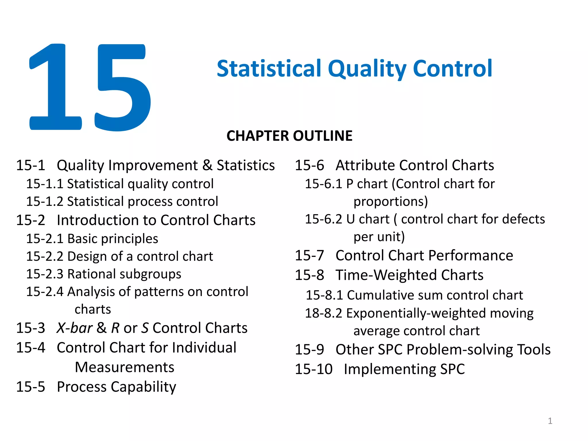
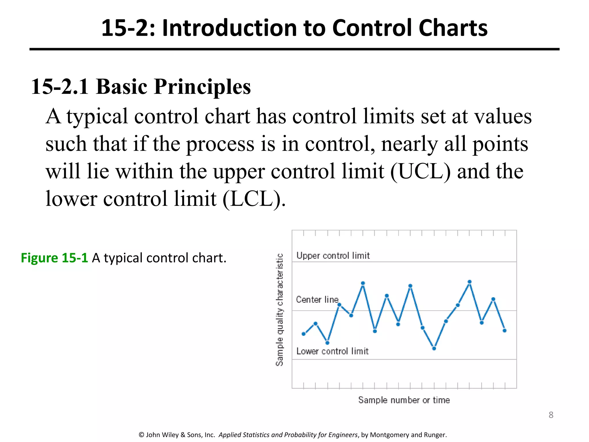
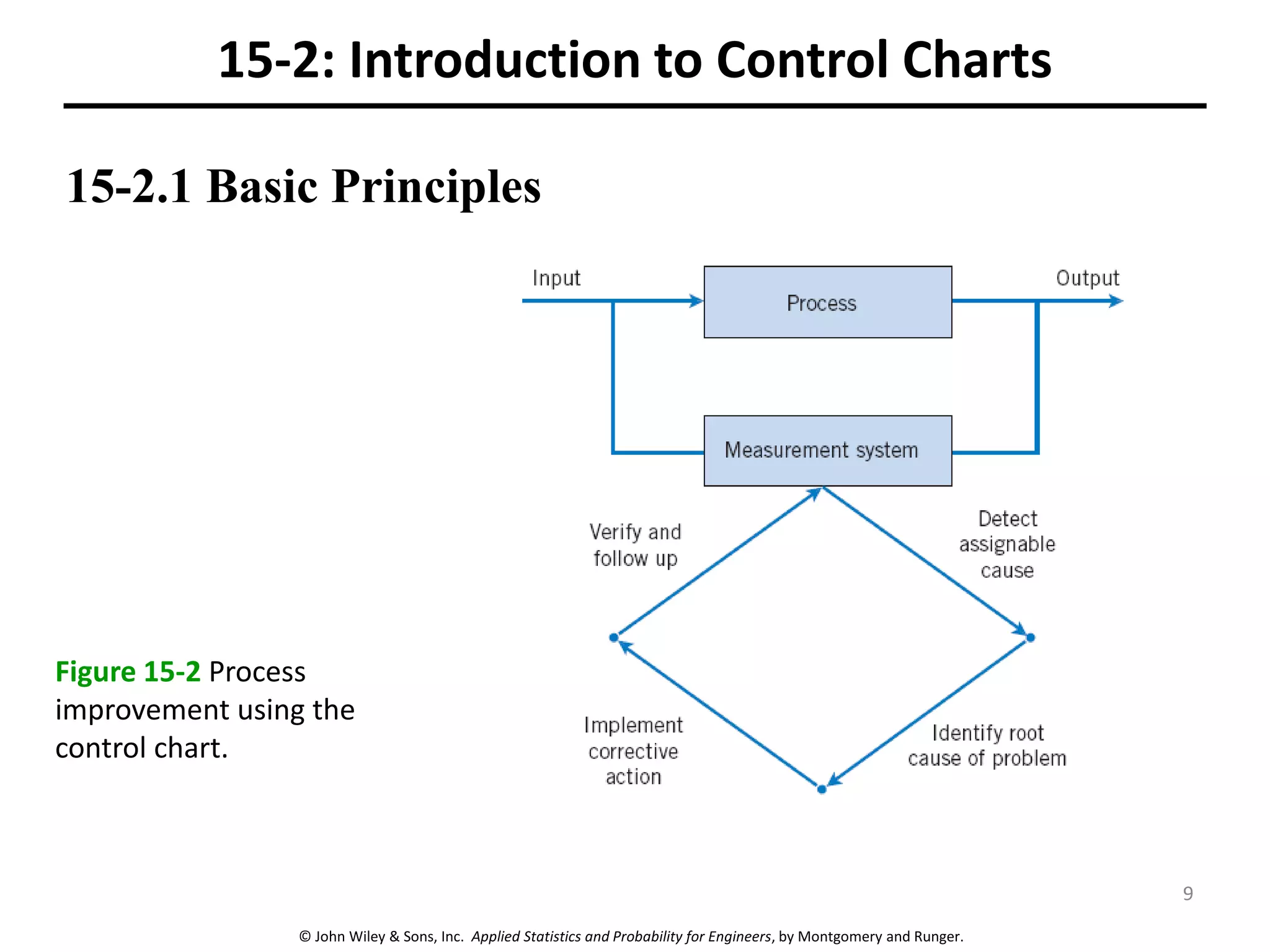
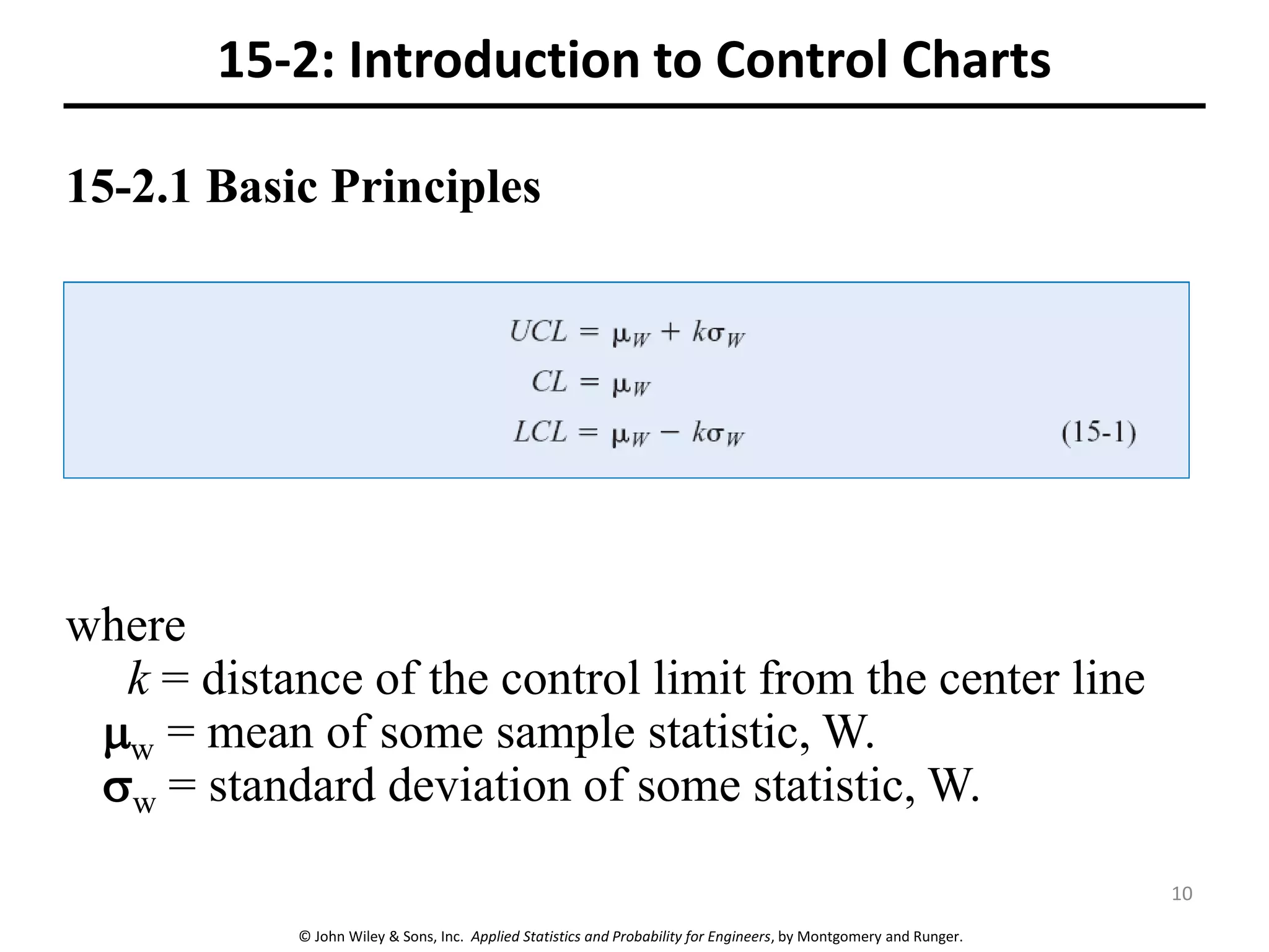
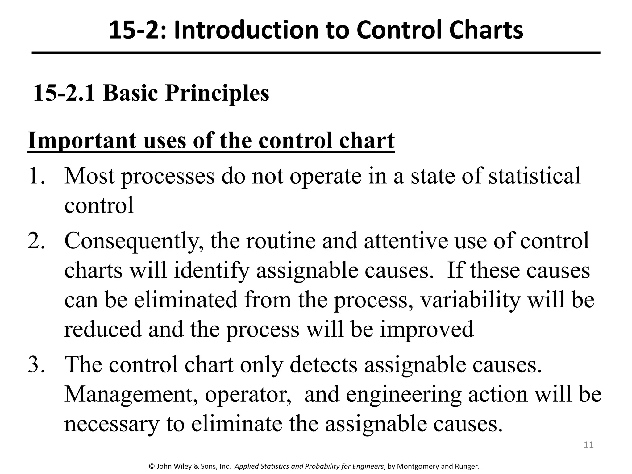
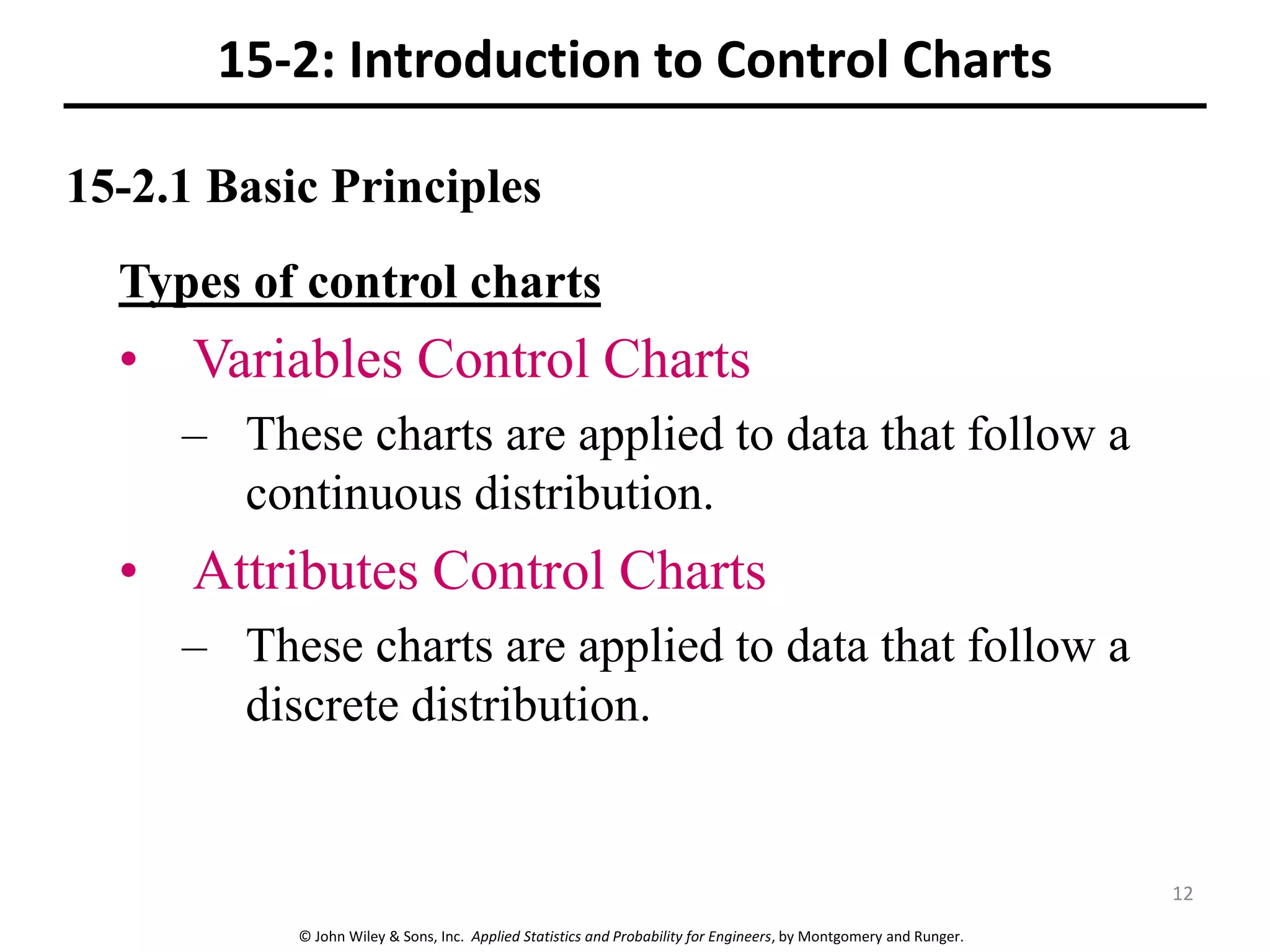
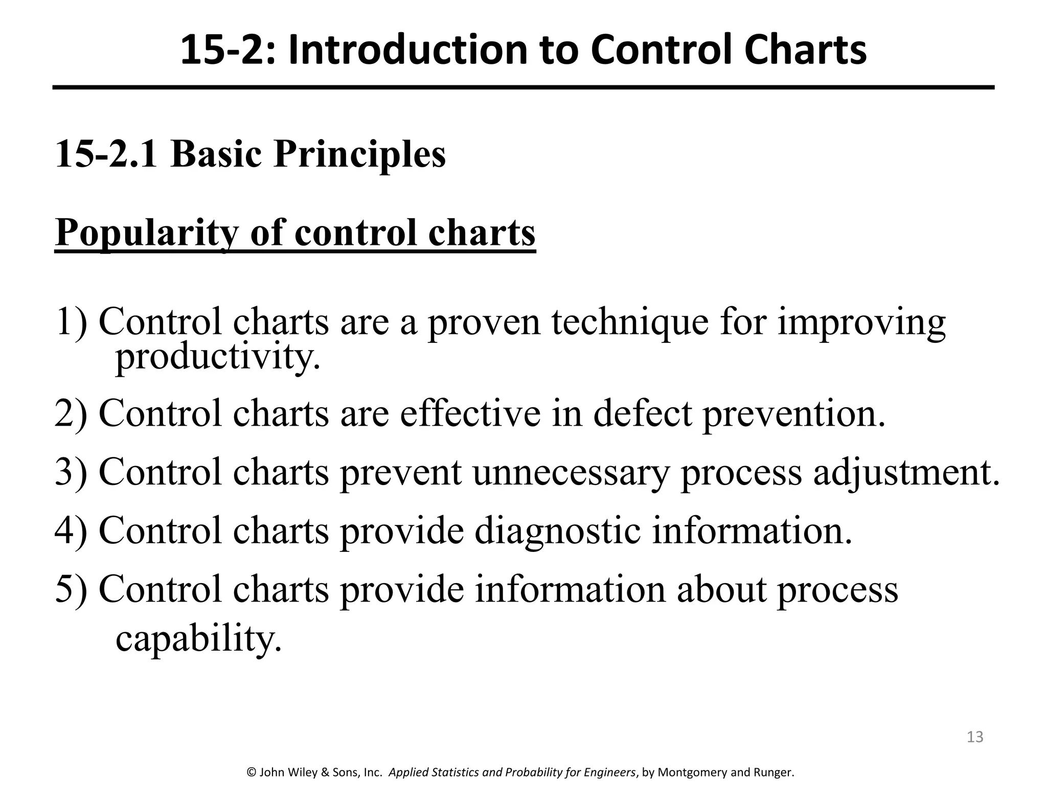
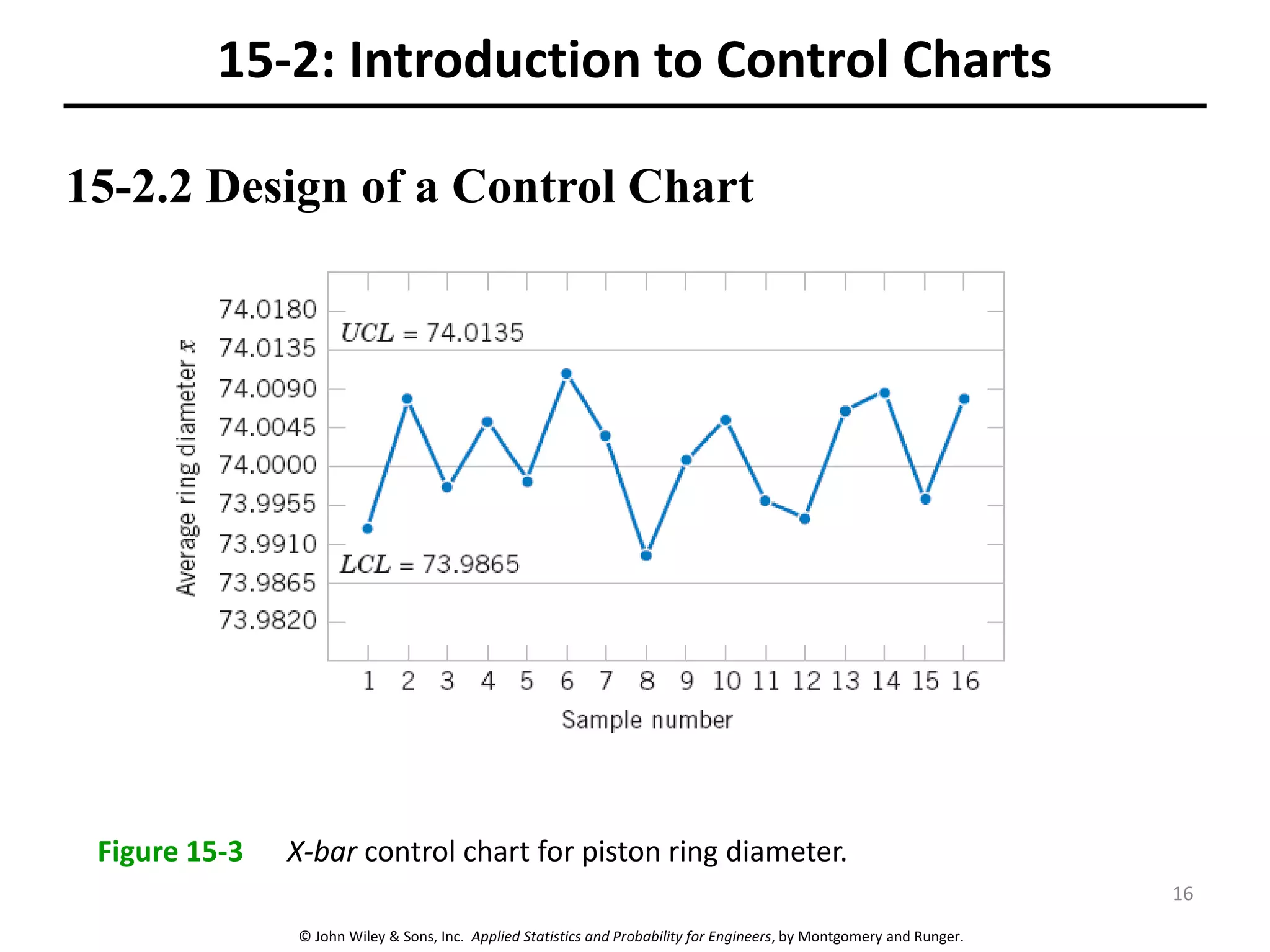
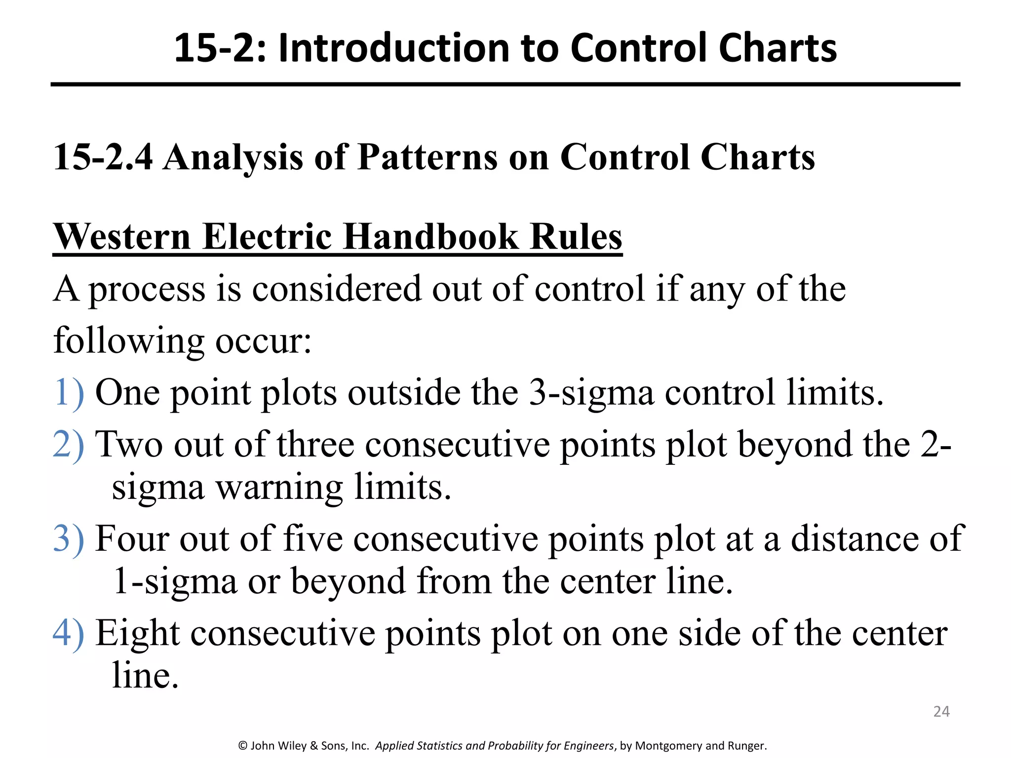
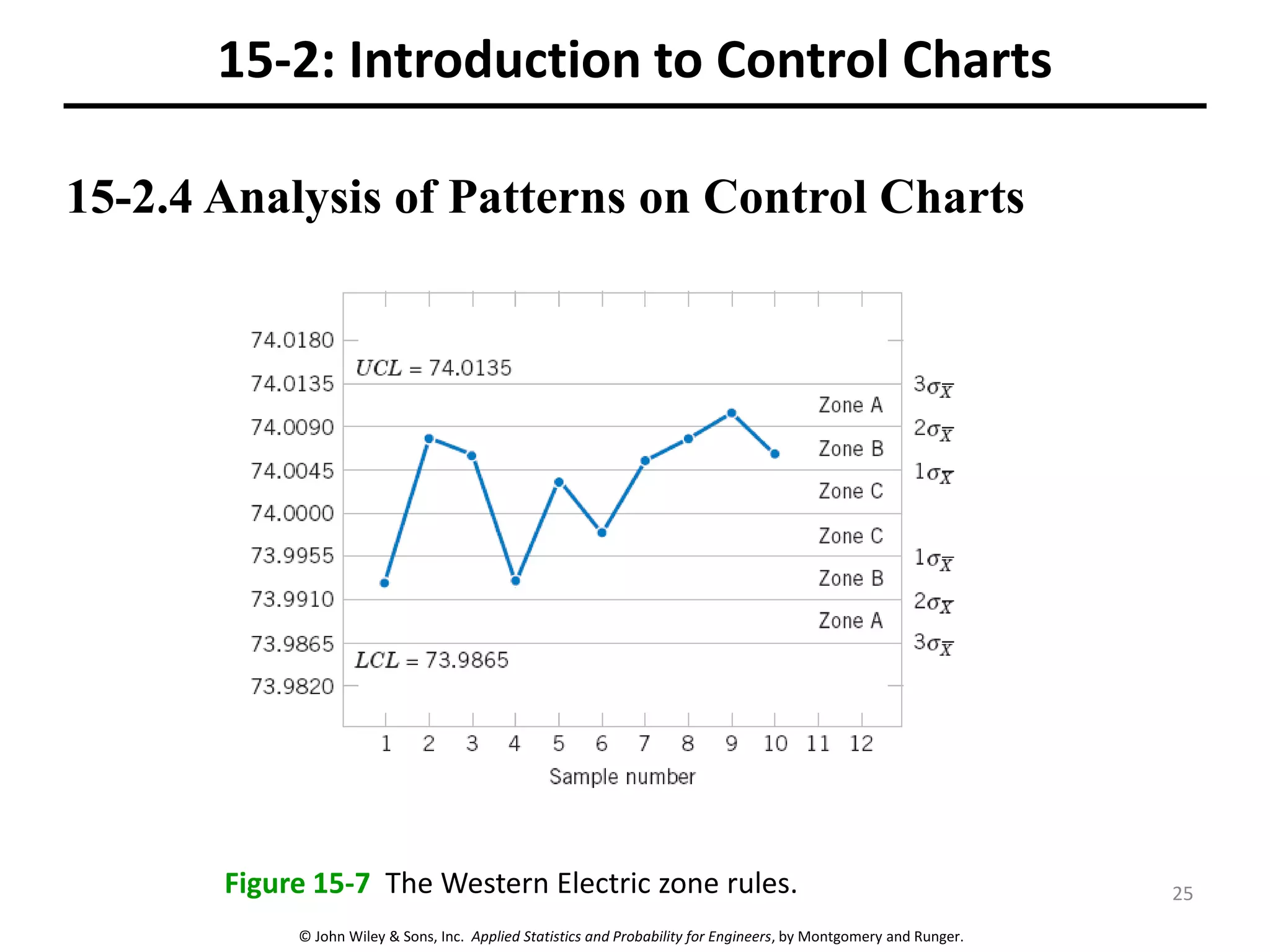
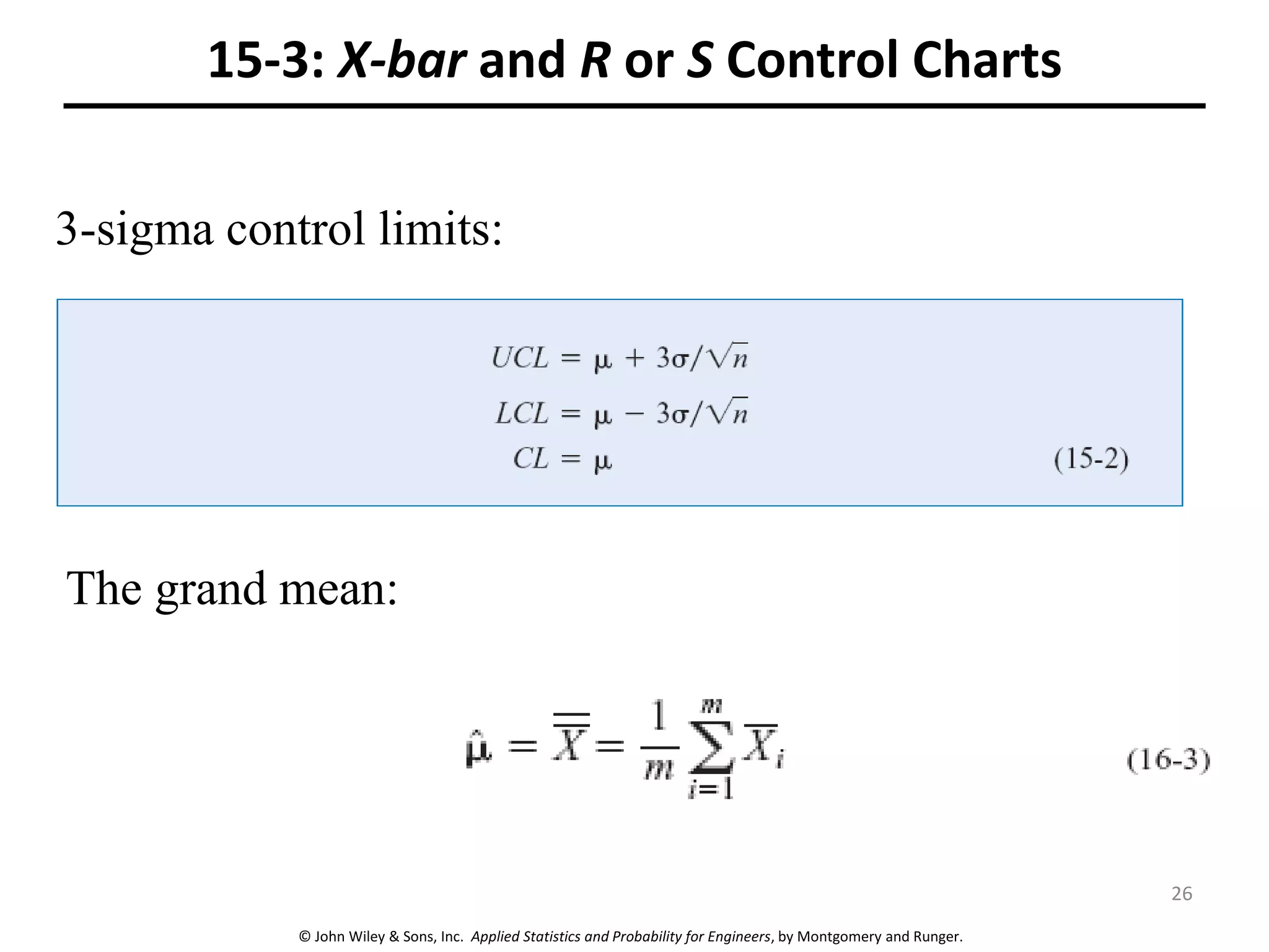
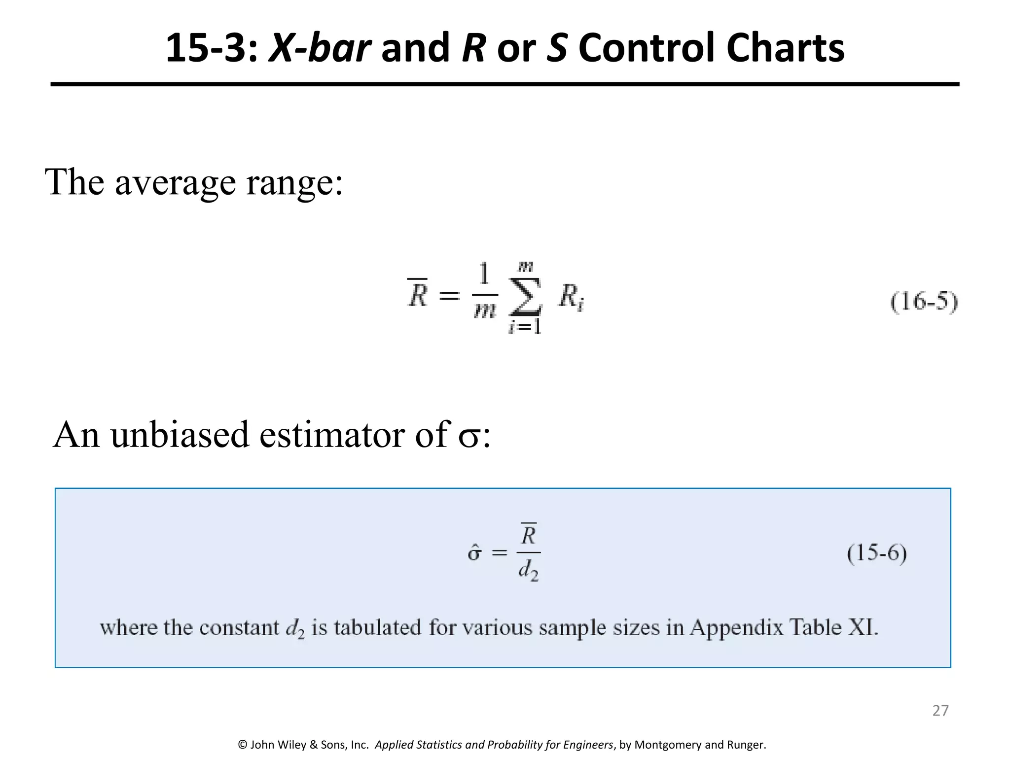
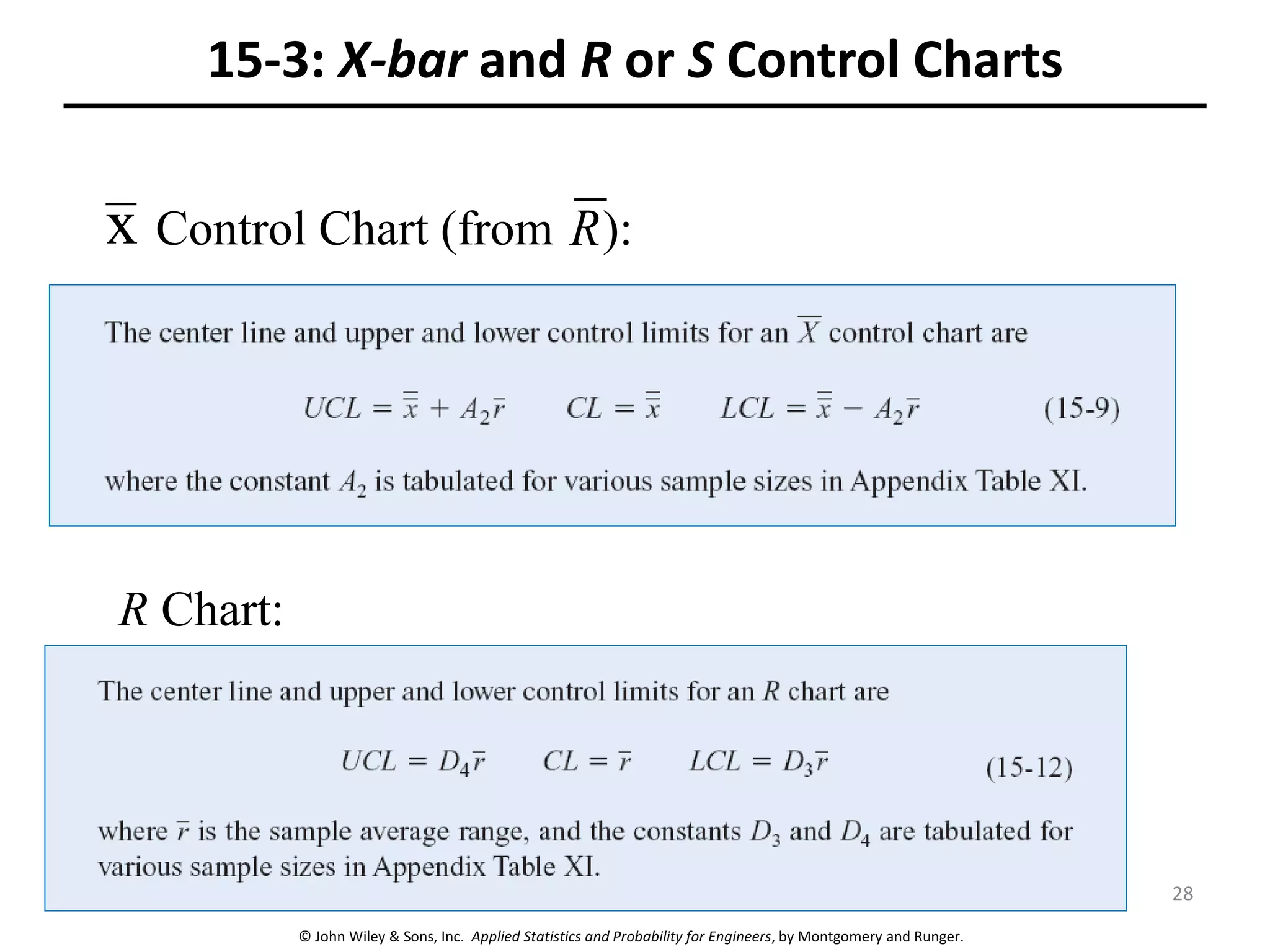
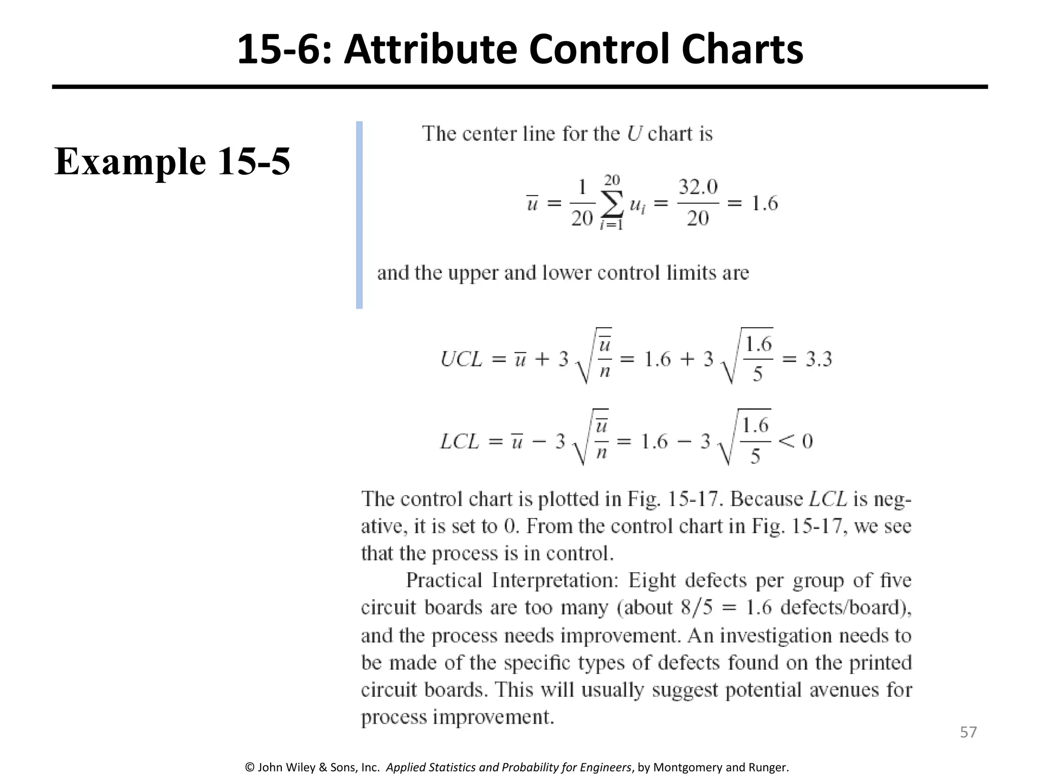
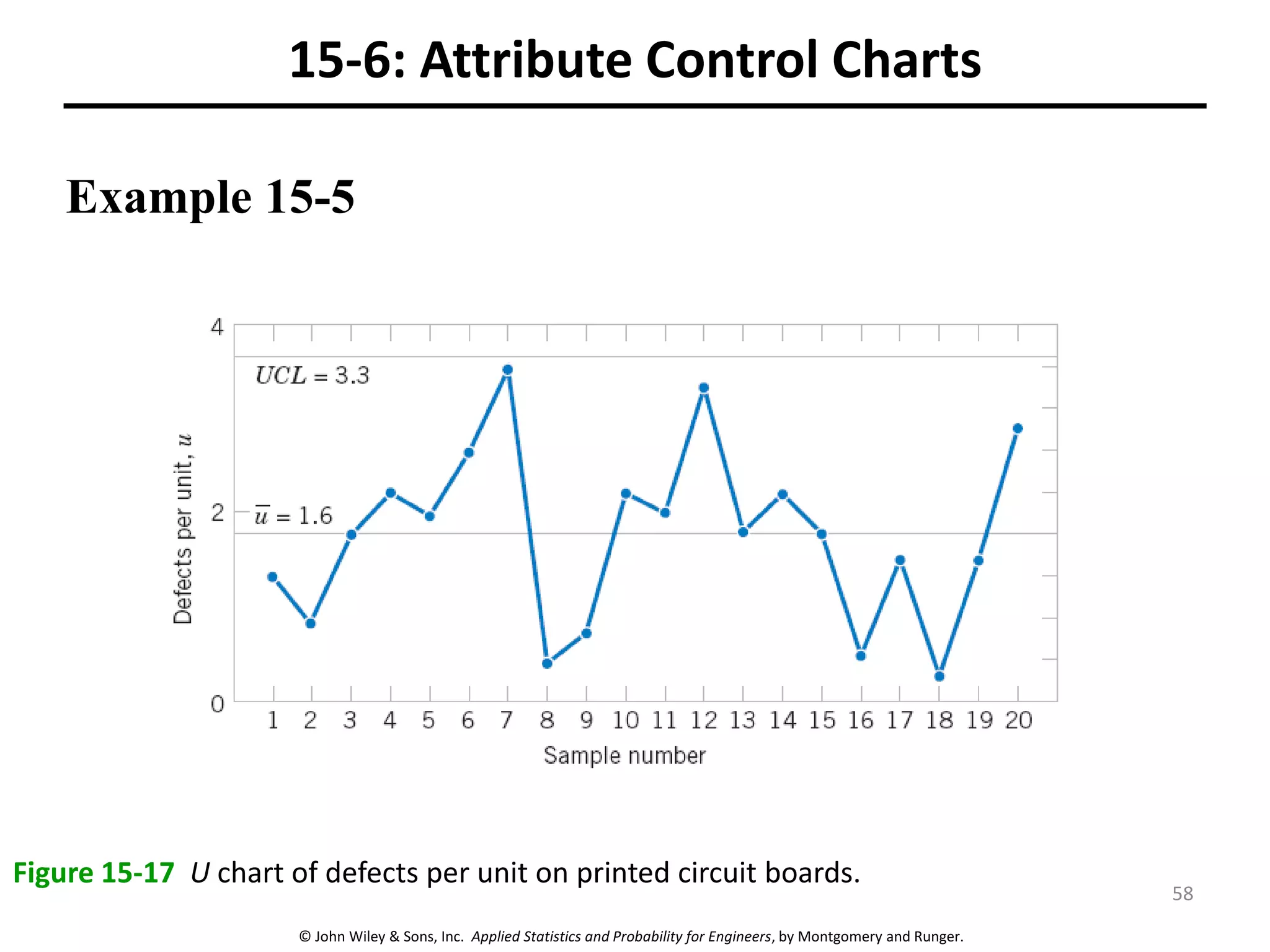
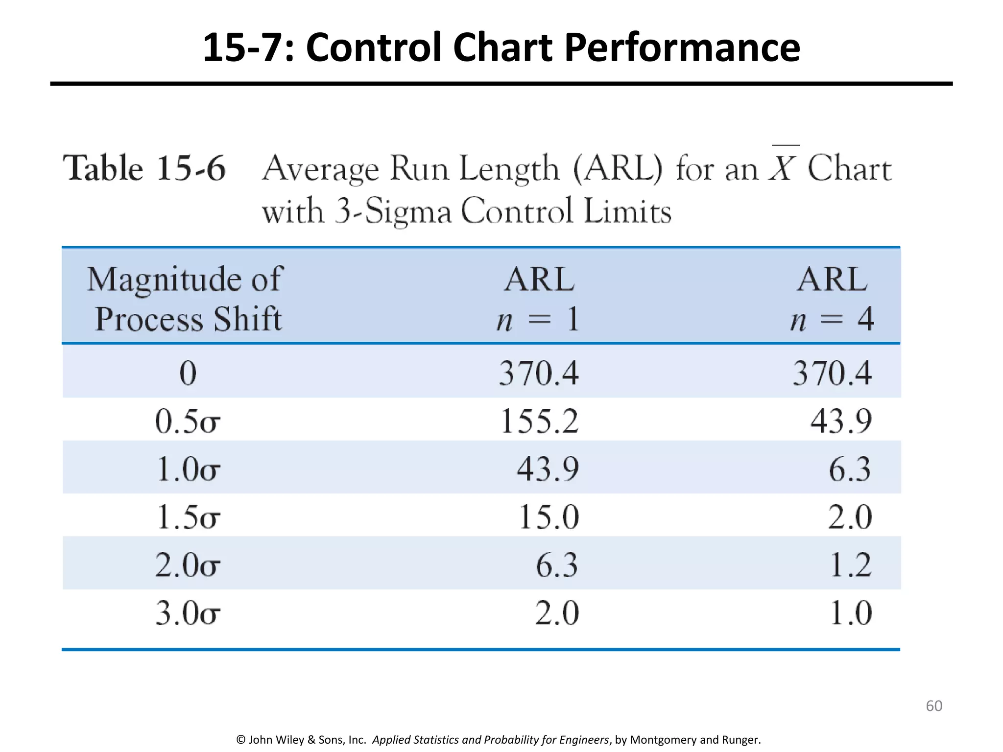
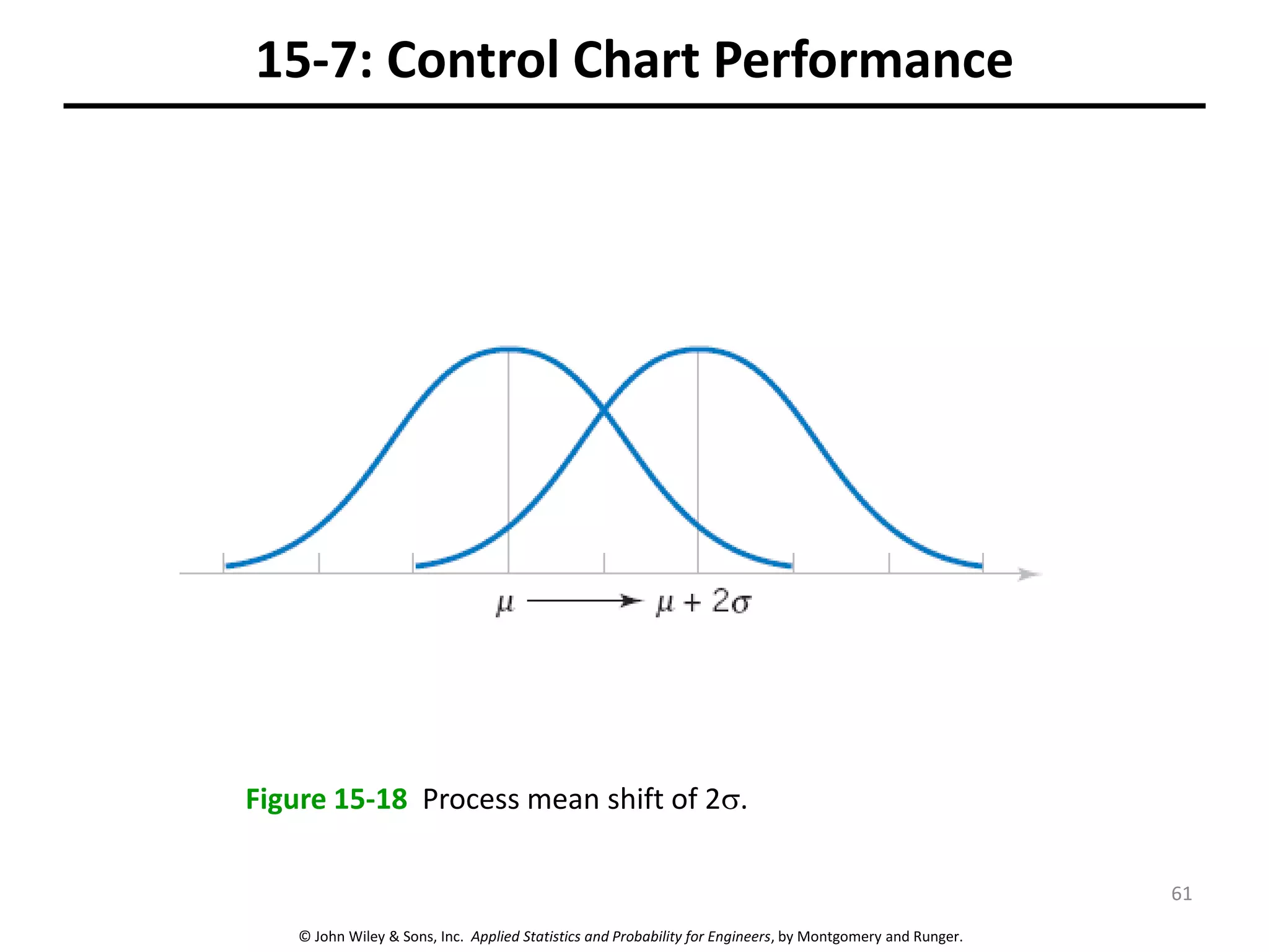
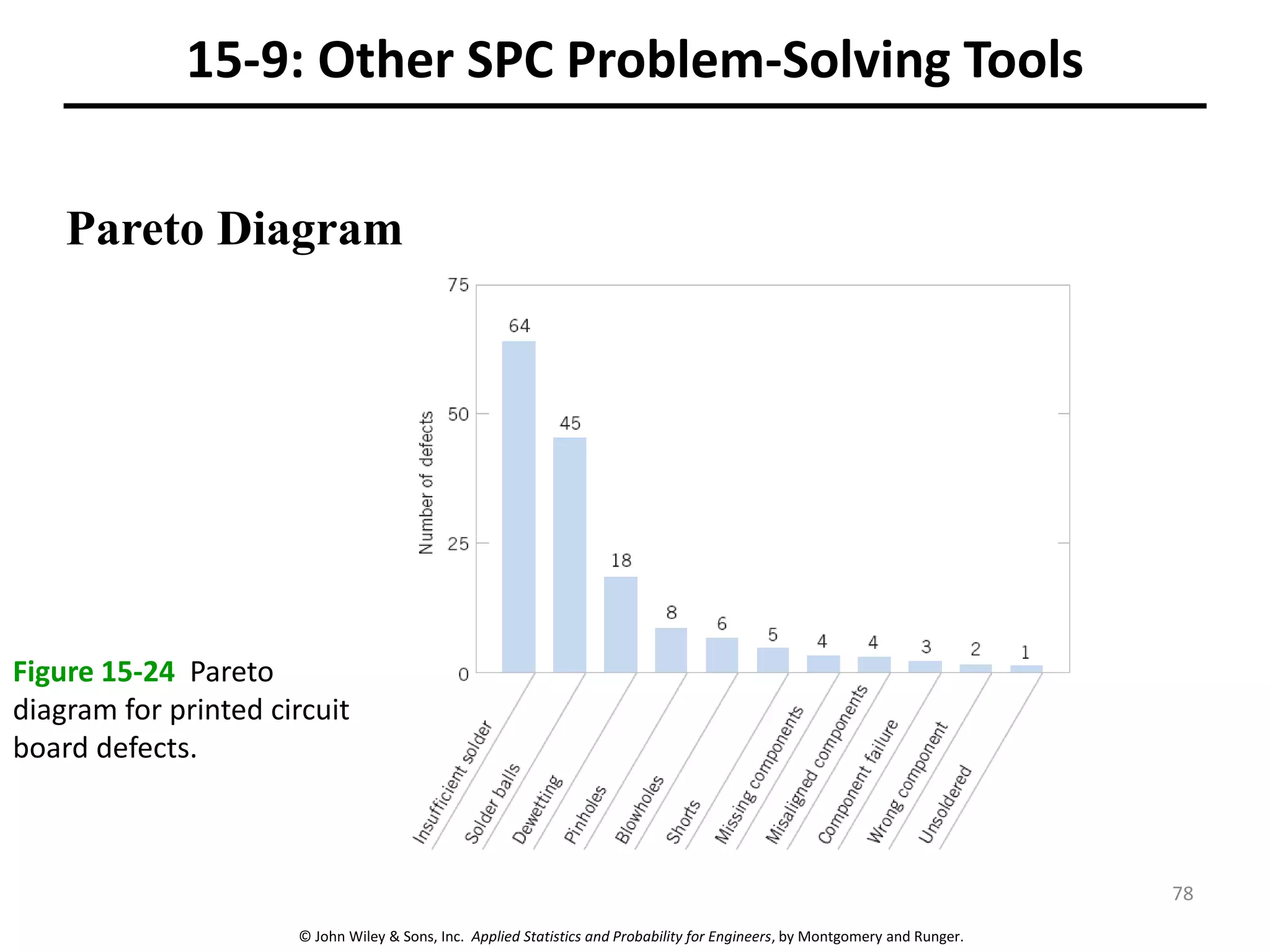
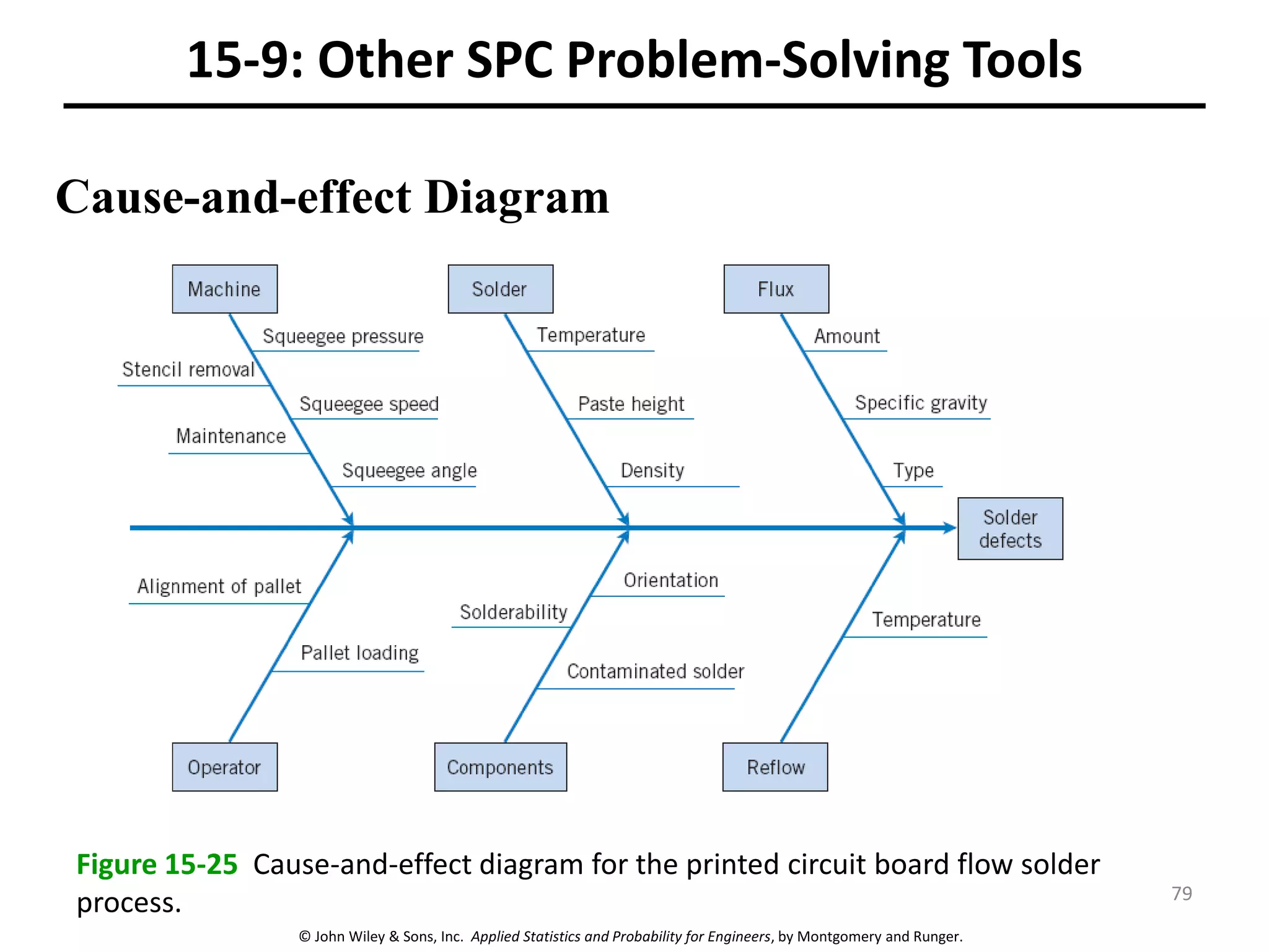
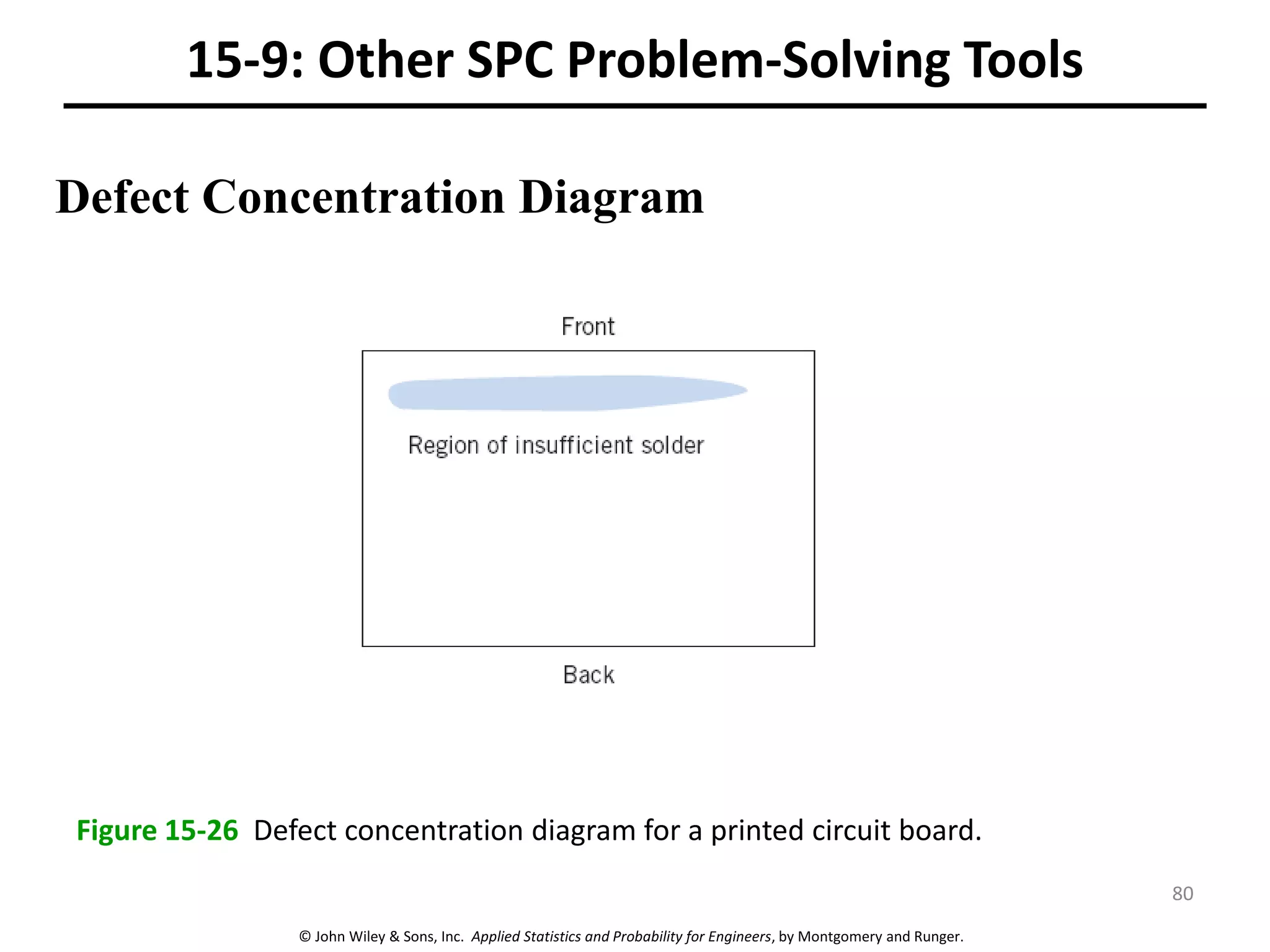
This chapter outline describes statistical quality control tools including control charts. Control charts are used to detect assignable causes of variation and improve processes. The chapter will cover both variables and attributes control charts, including X-bar and R charts to monitor process means and variability. It will also discuss rational subgrouping, pattern analysis, process capability analysis and calculation of control chart performance metrics. The goal is understanding how to construct and interpret different control charts and use statistical process control tools to improve quality.

1. 1
15 Statistical Quality Control
15-1 Quality Improvement & Statistics
15-1.1 Statistical quality control
15-1.2 Statistical process control
15-2 Introduction to Control Charts
15-2.1 Basic principles
15-2.2 Design of a control chart
15-2.3 Rational subgroups
15-2.4 Analysis of patterns on control
charts
15-3 X-bar & R or S Control Charts
15-4 Control Chart for Individual
Measurements
15-5 Process Capability
15-6 Attribute Control Charts
15-6.1 P chart (Control chart for
proportions)
15-6.2 U chart ( control chart for defects
per unit)
15-7 Control Chart Performance
15-8 Time-Weighted Charts
15-8.1 Cumulative sum control chart
18-8.2 Exponentially-weighted moving
average control chart
15-9 Other SPC Problem-solving Tools
15-10 Implementing SPC
CHAPTER OUTLINE

2. © John Wiley & Sons, Inc. Applied Statistics and Probability for Engineers, by Montgomery and Runger.
Learning Objectives for Chapter 15
After careful study of this chapter, you should be able to do the
following:
1. Understand the role of statistical tools in quality improvement.
2. Understand the different types of variability, rational subgroups, and how a
control chart is used to detect assignable causes.
3. Understand the general form of a Shewhart control chart and how to apply
zone rules (such as the Western Electric rules) and pattern analysis to detect
assignable causes.
4. Construct and interpret control charts for variables such as X-bar, R, S, and
individuals charts.
5. Construct and interpret control charts for attributes such as P and U charts.
6. Calculate and interpret process capability ratios.
7. Calculate the ARL performance for a Shewhart control chart.
8. Construct and interpret a cumulative sum and exponentially-weighted
moving average control chart.
9. Use other statistical process control problem-solving tools.
2

3. © John Wiley & Sons, Inc. Applied Statistics and Probability for Engineers, by Montgomery and Runger.
15-1: Quality Improvement and Statistics
• Definitions of Quality
Quality means fitness for use
- quality of design
- quality of conformance
Quality is inversely proportional to
variability.
3

4. © John Wiley & Sons, Inc. Applied Statistics and Probability for Engineers, by Montgomery and Runger.
15-1: Quality Improvement and Statistics
• Quality Improvement
Quality improvement is the reduction of
variability in processes and products.
Alternatively, quality improvement is also
seen as “waste reduction”.
4

5. © John Wiley & Sons, Inc. Applied Statistics and Probability for Engineers, by Montgomery and Runger.
15-1.2: Statistical Process Control
• Statistical process control is a
collection of tools that when used
together can result in process stability
and variance reduction
5

6. © John Wiley & Sons, Inc. Applied Statistics and Probability for Engineers, by Montgomery and Runger.
15-1.2: Statistical Process Control
The seven major tools are
1) Histogram
2) Pareto Chart
4) Cause and Effect Diagram
5) Defect Concentration Diagram
6) Control Chart
7) Scatter Diagram
8) Check Sheet
6

7. © John Wiley & Sons, Inc. Applied Statistics and Probability for Engineers, by Montgomery and Runger.
15-2: Introduction to Control Charts
• A process that is operating with only
chance causes of variation present is said
to be in statistical control.
• A process that is operating in the presence
of assignable causes is said to be out of
control.
• The eventual goal of SPC is the elimination
of variability in the process.
15-2.1 Basic Principles
7

8. © John Wiley & Sons, Inc. Applied Statistics and Probability for Engineers, by Montgomery and Runger.
15-2.1 Basic Principles
A typical control chart has control limits set at values
such that if the process is in control, nearly all points
will lie within the upper control limit (UCL) and the
lower control limit (LCL).
Figure 15-1 A typical control chart.
15-2: Introduction to Control Charts
8

9. © John Wiley & Sons, Inc. Applied Statistics and Probability for Engineers, by Montgomery and Runger.
15-2.1 Basic Principles
Figure 15-2 Process
improvement using the
control chart.
15-2: Introduction to Control Charts
9

10. © John Wiley & Sons, Inc. Applied Statistics and Probability for Engineers, by Montgomery and Runger.
15-2.1 Basic Principles
where
k = distance of the control limit from the center line
w = mean of some sample statistic, W.
w = standard deviation of some statistic, W.
15-2: Introduction to Control Charts
10

11. © John Wiley & Sons, Inc. Applied Statistics and Probability for Engineers, by Montgomery and Runger.
15-2.1 Basic Principles
Important uses of the control chart
1. Most processes do not operate in a state of statistical
control
2. Consequently, the routine and attentive use of control
charts will identify assignable causes. If these causes
can be eliminated from the process, variability will be
reduced and the process will be improved
3. The control chart only detects assignable causes.
Management, operator, and engineering action will be
necessary to eliminate the assignable causes.
15-2: Introduction to Control Charts
11

12. © John Wiley & Sons, Inc. Applied Statistics and Probability for Engineers, by Montgomery and Runger.
15-2.1 Basic Principles
Types of control charts
• Variables Control Charts
– These charts are applied to data that follow a
continuous distribution.
• Attributes Control Charts
– These charts are applied to data that follow a
discrete distribution.
15-2: Introduction to Control Charts
12

13. © John Wiley & Sons, Inc. Applied Statistics and Probability for Engineers, by Montgomery and Runger.
15-2.1 Basic Principles
Popularity of control charts
1) Control charts are a proven technique for improving
productivity.
2) Control charts are effective in defect prevention.
3) Control charts prevent unnecessary process adjustment.
4) Control charts provide diagnostic information.
5) Control charts provide information about process
capability.
15-2: Introduction to Control Charts
13

14. © John Wiley & Sons, Inc. Applied Statistics and Probability for Engineers, by Montgomery and Runger.
15-2.2 Design of a Control Chart
Suppose we have a process that we assume the true
process mean is  = 74 and the process standard
deviation is  = 0.01. Samples of size 5 are taken
giving a standard deviation of the sample average,
is
0045
.
0
5
01
.
0
n
x 




15-2: Introduction to Control Charts
14

15. © John Wiley & Sons, Inc. Applied Statistics and Probability for Engineers, by Montgomery and Runger.
15-2.2 Design of a Control Chart
• Control limits can be set at 3 standard
deviations from the mean in both directions.
• “3-Sigma Control Limits”
UCL = 74 + 3(0.0045) = 74.0135
CL= 74
LCL = 74 - 3(0.0045) = 73.9865
15-2: Introduction to Control Charts
15

16. © John Wiley & Sons, Inc. Applied Statistics and Probability for Engineers, by Montgomery and Runger.
15-2.2 Design of a Control Chart
15-2: Introduction to Control Charts
Figure 15-3 X-bar control chart for piston ring diameter.
16

17. © John Wiley & Sons, Inc. Applied Statistics and Probability for Engineers, by Montgomery and Runger.
15-2.2 Design of a Control Chart
• Choosing the control limits is equivalent to
setting up the critical region for hypothesis
testing
H0:  = 74
H1:   74
15-2: Introduction to Control Charts
17

18. © John Wiley & Sons, Inc. Applied Statistics and Probability for Engineers, by Montgomery and Runger.
15-2.3 Rational Subgrouping
15-2: Introduction to Control Charts
• Subgroups or samples should be selected
so that if assignable causes are present, the
chance for differences between subgroups
will be maximized, while the chance for
differences due to these assignable causes
within a subgroup will be minimized.
18

19. © John Wiley & Sons, Inc. Applied Statistics and Probability for Engineers, by Montgomery and Runger.
15-2.3 Rational Subgrouping
15-2: Introduction to Control Charts
Constructing Rational Subgroups
• Select consecutive units of production.
– Provides a “snapshot” of the process.
– Good at detecting process shifts.
• Select a random sample over the entire sampling
interval.
– Good at detecting if a mean has shifted
– out-of-control and then back in-control.
19

20. © John Wiley & Sons, Inc. Applied Statistics and Probability for Engineers, by Montgomery and Runger.
15-2.4 Analysis of Patterns on Control Charts
15-2: Introduction to Control Charts
• Look for “runs” - this is a sequence of
observations of the same type (all above the
center line, or all below the center line)
• Runs of say 8 observations or more could
indicate an out-of-control situation.
– Run up: a series of observations are increasing
– Run down: a series of observations are decreasing
20

21. © John Wiley & Sons, Inc. Applied Statistics and Probability for Engineers, by Montgomery and Runger.
15-2.4 Analysis of Patterns on Control Charts
15-2: Introduction to Control Charts
Figure 15-4 X-bar control chart.
21

22. © John Wiley & Sons, Inc. Applied Statistics and Probability for Engineers, by Montgomery and Runger.
15-2.4 Analysis of Patterns on Control Charts
15-2: Introduction to Control Charts
Figure 15-5 An X-bar chart with a cyclic pattern.
22

23. © John Wiley & Sons, Inc. Applied Statistics and Probability for Engineers, by Montgomery and Runger.
15-2.4 Analysis of Patterns on Control Charts
15-2: Introduction to Control Charts
Figure 15-6 (a) Variability with the cyclic pattern. (b) Variability with the cyclic pattern
eliminated. 23

24. © John Wiley & Sons, Inc. Applied Statistics and Probability for Engineers, by Montgomery and Runger.
15-2.4 Analysis of Patterns on Control Charts
15-2: Introduction to Control Charts
Western Electric Handbook Rules
A process is considered out of control if any of the
following occur:
1) One point plots outside the 3-sigma control limits.
2) Two out of three consecutive points plot beyond the 2-
sigma warning limits.
3) Four out of five consecutive points plot at a distance of
1-sigma or beyond from the center line.
4) Eight consecutive points plot on one side of the center
line.
24

25. © John Wiley & Sons, Inc. Applied Statistics and Probability for Engineers, by Montgomery and Runger.
15-2.4 Analysis of Patterns on Control Charts
15-2: Introduction to Control Charts
Figure 15-7 The Western Electric zone rules. 25

26. © John Wiley & Sons, Inc. Applied Statistics and Probability for Engineers, by Montgomery and Runger.
15-3: X-bar and R or S Control Charts
3-sigma control limits:
The grand mean:
26

27. © John Wiley & Sons, Inc. Applied Statistics and Probability for Engineers, by Montgomery and Runger.
15-3: X-bar and R or S Control Charts
The average range:
An unbiased estimator of :
27

28. © John Wiley & Sons, Inc. Applied Statistics and Probability for Engineers, by Montgomery and Runger.
15-3: X-bar and R or S Control Charts
Control Chart (from ):
R Chart:
x R
28

29. © John Wiley & Sons, Inc. Applied Statistics and Probability for Engineers, by Montgomery and Runger.
15-3: X-bar and R or S Control Charts
3-sigma control limits for S:
An unbiased estimator of :
29

30. © John Wiley & Sons, Inc. Applied Statistics and Probability for Engineers, by Montgomery and Runger.
15-3: X-bar and R or S Control Charts
S Chart:
Control Chart (from ):
x S
30

31. © John Wiley & Sons, Inc. Applied Statistics and Probability for Engineers, by Montgomery and Runger.
15-3: X-bar and R or S Control Charts
Example 15-1
31

32. © John Wiley & Sons, Inc. Applied Statistics and Probability for Engineers, by Montgomery and Runger.
32

33. © John Wiley & Sons, Inc. Applied Statistics and Probability for Engineers, by Montgomery and Runger.
15-3: X-bar and R or S Control Charts
Example 15-1
33

34. © John Wiley & Sons, Inc. Applied Statistics and Probability for Engineers, by Montgomery and Runger.
15-3: X-bar and R or S Control Charts
Example 15-1
Figure 15-8 and R control
charts for vane opening.
X
34

35. © John Wiley & Sons, Inc. Applied Statistics and Probability for Engineers, by Montgomery and Runger.
15-3: X-bar and R or S Control Charts
Example 15-1
35

36. © John Wiley & Sons, Inc. Applied Statistics and Probability for Engineers, by Montgomery and Runger.
15-3: X-bar and R or S Control Charts
Example 15-1
36

37. © John Wiley & Sons, Inc. Applied Statistics and Probability for Engineers, by Montgomery and Runger.
15-3: X-bar and R or S Control Charts
Example 15-1
Figure 15-9 The S control chart for vane opening.
37

38. © John Wiley & Sons, Inc. Applied Statistics and Probability for Engineers, by Montgomery and Runger.
15-3: X-bar and R or S Control Charts
Example 15-1
38

39. © John Wiley & Sons, Inc. Applied Statistics and Probability for Engineers, by Montgomery and Runger.
15-3: X-bar and R or S Control Charts
Example 15-1
Figure 15-10
The X-bar
and R control charts
for vane opening.
39

40. © John Wiley & Sons, Inc. Applied Statistics and Probability for Engineers, by Montgomery and Runger.
15-4: Control Charts for Individual Measurements
• What if you could not get a sample size greater than 1
(n =1)? Examples include
– Automated inspection and measurement technology
is used, and every unit manufactured is analyzed.
– The production rate is very slow, and it is
inconvenient to allow samples sizes of N > 1 to
accumulate before analysis
– Repeat measurements on the process differ only
because of laboratory or analysis error, as in many
chemical processes.
• The individual control charts are useful for samples of
sizes n = 1. 40

41. © John Wiley & Sons, Inc. Applied Statistics and Probability for Engineers, by Montgomery and Runger.
15-4: Control Charts for Individual Measurements
• The moving range (MR) is defined as the
absolute difference between two successive
observations:
MRi = |xi - xi-1|
which will indicate possible shifts or
changes in the process from one observation
to the next.
41

42. © John Wiley & Sons, Inc. Applied Statistics and Probability for Engineers, by Montgomery and Runger.
15-4: Control Charts for Individual Measurements
Individuals Control Chart
42

43. © John Wiley & Sons, Inc. Applied Statistics and Probability for Engineers, by Montgomery and Runger.
15-4: Control Charts for Individual Measurements
Interpretation of the Charts
• X Charts can be interpreted similar to X-bar charts. MR charts cannot be
interpreted the same as X-bar or R charts.
• Since the MR chart plots data that are “correlated” with one another, then
looking for patterns on the chart does not make sense.
• MR chart cannot really supply useful information about process variability.
• More emphasis should be placed on interpretation of the X chart.
43

44. © John Wiley & Sons, Inc. Applied Statistics and Probability for Engineers, by Montgomery and Runger.
15-5: Process Capability
• Process capability refers to the performance of
the process when it is operating in control.
• Two graphical tools are helpful in assessing
process capability:
• Tolerance chart (or tier chart)
• Histogram
44

45. © John Wiley & Sons, Inc. Applied Statistics and Probability for Engineers, by Montgomery and Runger.
15-5: Process Capability
Tolerance Chart
Figure 16-12 Tolerance diagram of
vane openings.
45

46. © John Wiley & Sons, Inc. Applied Statistics and Probability for Engineers, by Montgomery and Runger.
15-5: Process Capability
Histogram
Figure 15-13 Histogram for vane openings.
46

47. © John Wiley & Sons, Inc. Applied Statistics and Probability for Engineers, by Montgomery and Runger.
15-5: Process Capability
Process Capability Ratio
PCRk
47

48. © John Wiley & Sons, Inc. Applied Statistics and Probability for Engineers, by Montgomery and Runger.
15-5: Process Capability
Figure 15-14 Process Fallout and
the process capability ratio
(PCR).
48

49. © John Wiley & Sons, Inc. Applied Statistics and Probability for Engineers, by Montgomery and Runger.
15-5: Process Capability
Example 15-3
49

50. © John Wiley & Sons, Inc. Applied Statistics and Probability for Engineers, by Montgomery and Runger.
15-5: Process Capability
Figure 15-15 Mean of a six-sigma process shifts by 1.5 standard deviations.
50

51. © John Wiley & Sons, Inc. Applied Statistics and Probability for Engineers, by Montgomery and Runger.
15-6: Attribute Control Charts
15-6.1 P Chart (Control Chart for Proportions)
51

52. © John Wiley & Sons, Inc. Applied Statistics and Probability for Engineers, by Montgomery and Runger.
15-6: Attribute Control Charts
Example 15-4
52

53. © John Wiley & Sons, Inc. Applied Statistics and Probability for Engineers, by Montgomery and Runger.
15-6: Attribute Control Charts
Example 15-4
Figure 15-16 P chart for a ceramic substrate.
53

54. © John Wiley & Sons, Inc. Applied Statistics and Probability for Engineers, by Montgomery and Runger.
15-6: Attribute Control Charts
Example 15-4
54

55. © John Wiley & Sons, Inc. Applied Statistics and Probability for Engineers, by Montgomery and Runger.
15-6: Attribute Control Charts
15-6.2 U Chart (Control Chart for Defects per Unit)
55

56. © John Wiley & Sons, Inc. Applied Statistics and Probability for Engineers, by Montgomery and Runger.
15-6: Attribute Control Charts
Example 15-5
56

57. © John Wiley & Sons, Inc. Applied Statistics and Probability for Engineers, by Montgomery and Runger.
15-6: Attribute Control Charts
Example 15-5
57

58. © John Wiley & Sons, Inc. Applied Statistics and Probability for Engineers, by Montgomery and Runger.
15-6: Attribute Control Charts
Example 15-5
Figure 15-17 U chart of defects per unit on printed circuit boards.
58

59. © John Wiley & Sons, Inc. Applied Statistics and Probability for Engineers, by Montgomery and Runger.
15-7: Control Chart Performance
Average Run Length
• The average run length (ARL) is a very important
way of determining the appropriate sample size
and sampling frequency.
• Let p = probability that any point exceeds the
control limits. Then,
59

60. © John Wiley & Sons, Inc. Applied Statistics and Probability for Engineers, by Montgomery and Runger.
15-7: Control Chart Performance
60

61. © John Wiley & Sons, Inc. Applied Statistics and Probability for Engineers, by Montgomery and Runger.
15-7: Control Chart Performance
Figure 15-18 Process mean shift of 2.
61

62. © John Wiley & Sons, Inc. Applied Statistics and Probability for Engineers, by Montgomery and Runger.
15-8: Time-Weighted Charts
• The cusum chart incorporates all information in
the sequence of sample values by plotting the
cumulative sums of the deviations of the sample
values from a target value.
• If 0 is the target for the process mean, is the
average of the jth sample, then the cumulative
sum control chart is formed by plotting the
quantity
j
x
 



i
j
j
i X
S
1
0 )
(
15-8.1 Cumulative Sum Control Chart
62

63. © John Wiley & Sons, Inc. Applied Statistics and Probability for Engineers, by Montgomery and Runger.
63

64. © John Wiley & Sons, Inc. Applied Statistics and Probability for Engineers, by Montgomery and Runger.
15-8: Time-Weighted Charts
Figure 15-19 Plot of the
cumulative sum for the
concentration data, Table
15-7.
64

65. © John Wiley & Sons, Inc. Applied Statistics and Probability for Engineers, by Montgomery and Runger.
15-8: Time-Weighted Charts
Figure 15-20 The cumulative sum control chart. (a) The V-mask and scaling. (b) The cumulative
sum control chart in operation.
65

66. © John Wiley & Sons, Inc. Applied Statistics and Probability for Engineers, by Montgomery and Runger.
15-8: Time-Weighted Charts
CUSUM Control Chart
15-8.1 Cumulative Sum Control Chart
66

67. © John Wiley & Sons, Inc. Applied Statistics and Probability for Engineers, by Montgomery and Runger.
15-8: Time-Weighted Charts
Example 15-6
67

68. © John Wiley & Sons, Inc. Applied Statistics and Probability for Engineers, by Montgomery and Runger.
68

69. © John Wiley & Sons, Inc. Applied Statistics and Probability for Engineers, by Montgomery and Runger.
15-8: Time-Weighted Charts
Example 15-6
69

70. © John Wiley & Sons, Inc. Applied Statistics and Probability for Engineers, by Montgomery and Runger.
15-8: Time-Weighted Charts
Example 15-6
Figure 15-21 The CUSUM
status chart for Example
15-6.
70

71. © John Wiley & Sons, Inc. Applied Statistics and Probability for Engineers, by Montgomery and Runger.
15-8: Time-Weighted Charts
71

72. © John Wiley & Sons, Inc. Applied Statistics and Probability for Engineers, by Montgomery and Runger.
15-8: Time-Weighted Charts
15-8.2 Exponential Weighted Moving Average
Control Chart
72

73. © John Wiley & Sons, Inc. Applied Statistics and Probability for Engineers, by Montgomery and Runger.
15-8: Time-Weighted Charts
15-8.2 Exponential Weighted Moving Average
Control Chart
73

74. © John Wiley & Sons, Inc. Applied Statistics and Probability for Engineers, by Montgomery and Runger.
15-8: Time-Weighted Charts
15-8.2 Exponential Weighted Moving Average
Control Chart
Figure 15-22 EWMAs with λ=0.8 and λ=0.2 show a compromise between a smooth curve
and a response to a shift
74

75. © John Wiley & Sons, Inc. Applied Statistics and Probability for Engineers, by Montgomery and Runger.
15-8: Time-Weighted Charts
EWMA Control Chart
15-8.2 Exponential Weighted Moving Average
Control Chart
75

76. © John Wiley & Sons, Inc. Applied Statistics and Probability for Engineers, by Montgomery and Runger.
15-8: Time-Weighted Charts
Example 15-7
76

77. © John Wiley & Sons, Inc. Applied Statistics and Probability for Engineers, by Montgomery and Runger.
15-8: Time-Weighted Charts
15-8.2 Exponential Weighted Moving Average
Control Chart
Figure 15-23 EWMA control chart for the Chemical Process Concentration Data from
Minitab.
77

78. © John Wiley & Sons, Inc. Applied Statistics and Probability for Engineers, by Montgomery and Runger.
15-9: Other SPC Problem-Solving Tools
Pareto Diagram
Figure 15-24 Pareto
diagram for printed circuit
board defects.
78

79. © John Wiley & Sons, Inc. Applied Statistics and Probability for Engineers, by Montgomery and Runger.
15-9: Other SPC Problem-Solving Tools
Cause-and-effect Diagram
Figure 15-25 Cause-and-effect diagram for the printed circuit board flow solder
process. 79

80. © John Wiley & Sons, Inc. Applied Statistics and Probability for Engineers, by Montgomery and Runger.
15-9: Other SPC Problem-Solving Tools
Defect Concentration Diagram
Figure 15-26 Defect concentration diagram for a printed circuit board.
80

81. © John Wiley & Sons, Inc. Applied Statistics and Probability for Engineers, by Montgomery and Runger.
15-10: Implementing SPC
• Strategic Management of Quality
• Deming’s 14 points
81

82. © John Wiley & Sons, Inc. Applied Statistics and Probability for Engineers, by Montgomery and Runger.
Important Terms & Concepts of Chapter 15
ARL
Assignable causes
Attributes control charts
Average run length
C chart
Cause-and-effect diagram
Center line
Chance causes
Control chart
Control limits
Cumulative sum control
chart
Defect concentration
diagram
Defects-per-unit chart
Deming’s 14 points
Exponentially-weighted
moving average
control chart (EWMA)
False alarm
Fraction-defective control
chart
Implementing SPC
Individuals control chart
(X chart)
Moving range
NP chart
P chart
Pareto diagram
PCR
PCRk
Problem-solving tools
Process capability
Process capability ratio
Quality control
R chart
Rational subgroup
Run rule
S chart
Shewhart control chart
Six-sigma process
Specification limits
82