1453244885.pptxsDVswvfsdvsdvsdvsdvVSDvsdvsvsdv

§c o n t r o l s t a t i o n
Fundamentals of Instrumentation
& Process Control
Interactive Training Workshop

I Fundamentals of Instrumentation & Control
«$control s t a t i o n
2
Copyright© 2007 Control Station, Inc. All Rights Reserved
I'M GAC Ff
OM
"TRA1NiNG
l GOT A. B!
G
G l N D E ,

I Introduction to Process Control
3
A common misconception in process control is that it is all
about the controller -that you can force a particular
process response just by getting the right tuning
parameters.
In reality, the controller is just a partner. A
process will respond to a controller's commands only in
the manner which it can. To understand process
control you must understand the other partners as well:
sensors, final control elements and the process itself.
All of these determine what type of response the controller
is capable of extracting out of the process. It is not the
other way around.

I Outline of the
Course
Disturbances
Set Point
(SP)
Resource
[Steam)
lnput(s)
(Cold Water]
-
Controller Output
(CO) i ',
- -
Manipulated Variable
(MV)
(Steam Pressure]
Output
[Hot Water]
Algorithm .
c1-'
4
-- I
Controller
i
•
Final Control
Element
Prooess
,.._,
Prooess Variable
(PV)
[Temperature)
.
.
..
L
Sensor

I Introduction to Process Control
5
• Objectives:
■ Why do we need process control?
■ What is a process?
■ What is process control?
■ What is open loop control?
■ What is closed loop control?
■ What are the modes of closed loop control?
■ What are the basic elements of process control?

I Motivation for Automatic Process Control
6
• Safety First:
■ people, environment, equipment
• The Profit Motive:
■ meeting final product specs
■ minimizing waste production
■ minimizing environmental impact
■ m1■
n1•
m1•
z1•
ng energy use
■ maximizing overall production rate

I "Loose" Control Costs
Money
i
65•··-· - · - - ,. ·-··-·-··-·7 operatin? constraint·························
0
7
- 6 0 1
0
a.
Q)
0
E
a.. 55
Cf)
o6
> SP
--
a..
45. ··-·- - · - - ·
i
40 poor control= large variation in PV --· b y C o ir ::i n
:.
• All Rights
Reserved
1 set point far
from profit
constraint
50 100 150 200
Time
• It takes more processing to remove impurities, so greatest
profit is to operate as close to the maximum impurities
constraint as possible without going over
• It takes more material to make a product thicker, so greatest
profit is to operate as close to the minimum thickness
constraint as possible without going under

I "Tight" Control is More
Profitable
i
+-'
-
0
...
.
c.
.
.Q
...
.)
0
E
65. ····--··----:-··-··············+-···· operating c o n s t r a i n t - - set point near
r
6 0 - , - - - - ......--------1
----:
----1 profit
constraint
0
)
fu
SP
i 5 0 + - - - - - - - - -·--····+···-····· -
a..
45
_··-·· tight co trol =
smauvariatiomn PV
40
··-·-··-··-··-·-+·-·-··--· : ·
8
;·:· -:;·
50
i
100
;;:· ;:;:,·:-··:1ightsReserved
i
150 200
Time
• A well controlled process has less variability in the
measured process variable (PV), so the process can be
operated close to the maximum profit constraint.

I Terminology for Home Heating Control
9
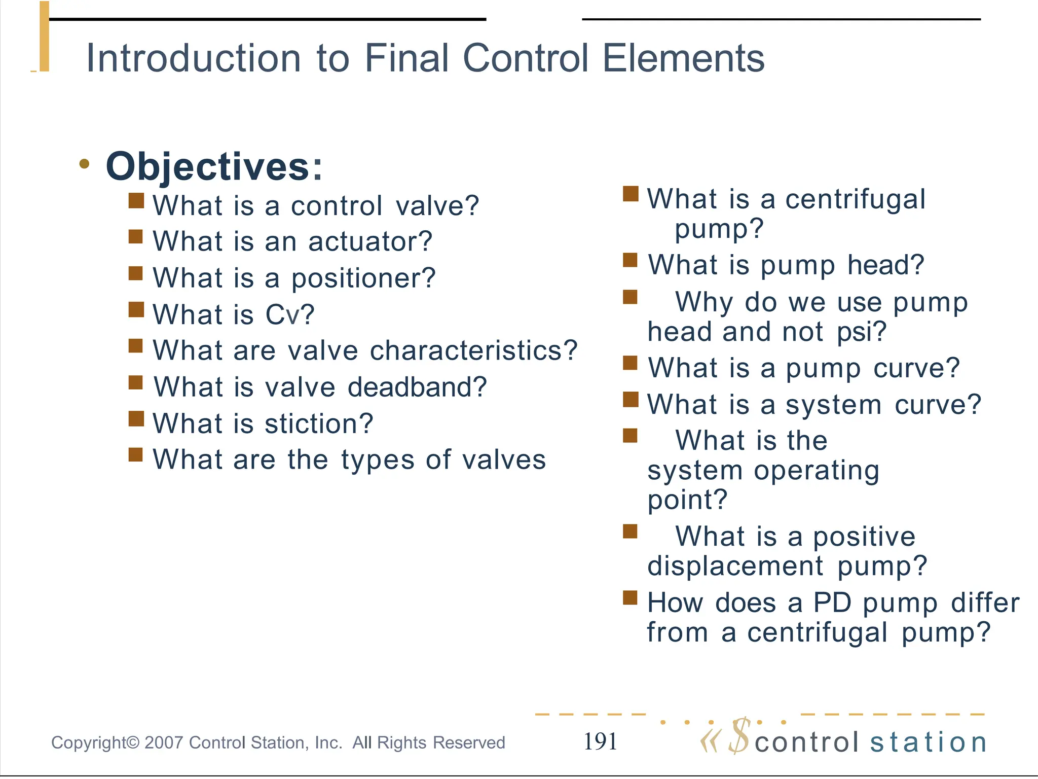
■ Control Objective
■ Measured Process Variable (PV)
■ Set Point (SP)
■ Controller Output (CO)
■ Manipulated Variable
■ Disturbances (D) thermostat
controller
set point -
I
I
•@+- ----
E]
I
control
1
signal :
temperature
sensor/transmitter
furnace
valve
Copyright© 2007 by Control Station, Inc. All Rights
Reserved
heat loss
(disturbance)

I What is Process Control
• Terminology:
■ The manipulated variable (MV) is a measure of resource
being fed into the process, for instance how much
thermal energy.
■ A final control element (FCE) is the device that
changes the value of the manipulated variable.
■ The controller output (CO) is the signal from the
controller to the final control element.
■ The process variable (PV) is a measure of the process
output that changes in response to changes in the
manipulated variable.
■ The set point (SP) is the value at which we wish to
maintain the process variable at.
Copyright© 2007 Control Station, Inc. All Rights Reserved 1 «$control s t a t i o n

I What is a Process
• A process is broadly defined as an
operation that uses resources to
transform inputs into outputs.
• It is the resource that provides the energy
into the process for the
transformation to occur.
lnput(s)
'
.
Resource - - - - i - . . i Process 1 - - - ► : Output

I What is a Process
12
0•100
P9C
ST-1
OOtllltNSAl[ - - - - - - - C : , . : 1 - - - - - I
R£Tl.f(N
118XX
50-300'F'
C O L D - - - - - - <
/ATER
PP-I00
CONDENSATE
RETURN
hP·IOl
Process
HOT
WATER

I What is a Process
13
• Each process exhibits a particular dynamic (time
varying) behavior that governs the
transformation.
■That is, how do changes in the resource or inputs
over time affect the transformation.
• This dynamic behavior is determined by the
physical properties of the inputs, the
resource, and the process
itself.

I What is a Process
14
• Can you identify some of the elements that
will determine the dynamic
properties of this process?
COLD
w • r t P . - - - - - <

15
• Process control is the act of controlling a final
control element to change the manipulated
variable to maintain the process variable at a
desired set point.
■A corollary to our definition of process control is a
controllable process must behave in a
predictable manner.
■ For a given change in the manipulated variable, the
process variable must respond in a predictable
and consistent manner.

Resource
[Steam)
lnput(s)
(Cold Water]
A controlled change
in the Final Control
Element Final Control
Element
(MV)
[Steam Pressure]
Ii'" ...
16
HP -.01
Proces
s
Output
[Hot Water]
Process Variable
(PV)
[Temperature]
.
Results in a
predictable change in
the Process Variable
Sensor

.,.
.
P!IC
ReSOtl'te
v>!/.x
Final
Comol
EJemefi
Manipwad Variable
Opening Velve
=
Increase in
T7
Process
Variable
COI.D
'lll<TER-- - - - - - !
PP-100
CO IOEl ATE - - frl-(]Hltil::
RETI.IRN
17
HOT
WATER

Section Assessment:
Basic T
errmtnoEogy Assess1
1
1
1tent
18

I What is Open Loop Control
19
• In open loop control the controller output
is not a function of the process variable.
■In open loop control we are not concerned that
a particular set point be maintained, the
controller output is fixed at a value until it is
changed by an operator.
■ Many processes are stable in an open loop control
mode and will maintain the process variable
at a value in the absence of a disturbances.
■ Disturbances are uncontrolled changes in the
process inputs or resources.

I What is Open Loop
Control
Disturbances
Resource
[Steam]
lnput(s)
[Cold Water]
Set Point
(SP) - - - - i
Controller
Controller Output
(CO)
/
(MV)
[Steam Pressure]
Output
[Hot Water)
Final Control
Element
-
20
......
Process
-'
·
Process Variable
(PV)
[Temperature)
-
Sensor

I What is Open Loop Control
21
• Can you think of processes in which open
loop control is
sufficient?
IO )OO•f
•
T
•
I
PSV
"'
50'11,0pen
1 1 0 ?
Process
Variable
rl.P-101
Proces
s

I What is Closed Loop Control
22
• In closed loop control the controller output
is determined by difference between the
process variable and the set point.
Closed loop control is also called feedback or
regulatory control.
■The output of a closed loop controller is a function of
the error.
■ Error is the deviation of the process variable from
the set point and is defined as
E = SP - PV.

Disturbances
Resource
[Steam)
lnput(s)
[Cold Water]
Set Point + Error Algorithm
(SP) , _
23
1 - 1 - ------,
Controller
Controller Output
(CO)
Final Control
Element
(MV)
(Steam Pressure]
H,.P-1'1
t
Process
Output
[Hot Water]
Process Variable
(PV)
[Temperature]
S
e
n
s
o
r

• From the controllers
perspective the
process encompasses
the RTD, the steam
control valve, and
signal processing
of the PV and
CO values.
co
"
24
• PV

I What are the Modes of Closed Loop Control
25
• Closed loop control can be, depending on the
algorithm that determines the controller
output:
■ Manual
■ On-Off
■ PIO
■ Advanced PIO (ratio, cascade, feedforward)
■ or Model Based

Manual Control
26
• In manual control an operator directly
manipulates the controller output to the
final control element to
maintain a set point.
ReSOIJ'te .,,.,
Sl(AM
SUPPI..Y VIY.>
'1l"o : -· - - : - " - . . k i m = l - -----' -- c o - -+ 1 • SP
A. •
PV

On-Off Control
27
• On-Off control provides a controller output
of either on or offin response to
error.
• t-------'-P V - -'--- ,
S P

On-Off Control Deadband
28
• Upon changing the direction of the controller
output, deadband is the value that must be
traversed before the controller output will
change itsdirection again.
PV > (SP + 1/2Dea<l>and) i
COOf
f
I
I
I ,.....-:===,._.
_
I
I
,,
SP
Dea<lI
>an
d
I
I
L - - - - - - - = - - - - - -
t
I
: PV < (SP - 1/2
Deadbend)
coon

PIO Control
29
• PID control provides a controller output that
modulates from 0 to 100°/o in response to
error.
R&SOll'C& VAXX
S1£MI
SUPP.Y
srx,
VAXX
CONO!:tfSArC.
f'{ElUUf
VS<X co
PO SP
A
l
SO•JQCl'r
Tl
.P
.O
.V
•
• PV
COLI>
WAfE((
Pfl·IOO
CONOOlSATE
RITUR!l
I
l•2.
WA'T
"E".R
liP·101
Proces
s

Cycle Time is the time base of the
signal the final control element will
receive from the controller. The PIO
controller determines the final signal
to the controller by multiplying the
cycle time by the output of the PIO
algorithm.
I
30
What are the Modes of Closed Loop
Control
Time Proportion Control
• Time proportion control is a variant of PID control that
modulates the on-off time of a final control element that
only has two command positions.
■ To achieve the effect of PIO
control the switching
frequency
of the device is modulated in
response to error. This is
achieved by introducing the
concept of cycle time.
100'!(,co
70'!bCO
so,r,co
to to+10sec to+20sec to+30sec to+40sec

Cascade Control
• Cascade control uses the output of a primary (master
or outer) controller to
manipulate the set point of a secondary (slave or inner)
controller as if the slave controller were the final
control element.
Re
JSlewn
)
l"""t(s)
(Coldwa:e,J
F>rirnory
eoo.-
au,pu,
(CO)Sot Point
(SP)
- • ' Y
Con"°1et OIApul
Algo<illlmH--"'(00=)-
Fll"IDIConiro1
-
-
Marnpulatcd
Variabl8
(MV)
fSte.,m PrKSuret
31
, - J ' - - ,
(PV1t
Socond,,y
ProoeuVa,fabfe
JSi.eamP.-e j

I
32
What are the Modes of Closed Loop Control
Cascade Control
co Secondary
Comoler
co
v
e
x
x FCE
Primary
comoler
COLO
WATER► -
PP•IOO
CON>ENSATE◄--fil--0-,-
RETURN sT-
••
2
1
Hf>•IOI
Proces
s

I Basic Elements of Process Control
33
• Controlling a process requires knowledge of
four basic elements, the process itself, the
sensor that measures the process
value, the final control element that changes
the manipulated variable, and the
controller .
..
Process

Section Assessment:
Basic Process Control
Assessment
34

I Understanding Dynamic Process Behavior
35
What We Will Learn in ThEs Secttton
• Dynamic Process Behavior - What It Is & Why We
Care
• What a FOPDT Dynamic Model Represents
• Analyzing Step Test Plot Data to Determine FOPDT
Dynamic Model Parameters
• Process Gain, Time Constant & Dead Time
■ How To Compute Them From Plot Data
■ How to Use Them For Controller
Design and Tuning
• How to Recognize Nonlinear Processes

I Dynamic Process Behavior and Controller
Tuning
36
• Consider cruise control for a car vs a truck
■ how quickly can each accelerate or decelerate
■ what is the effect of disturbances (wind, hills, etc.)
• Controller (gas flow) manipulations required to
maintain set point velocity in spite of disturbances
(wind, hills) are different for a car and truck because the
dynamic behavior of each "process" is different
• Dynamic behavior how the measured process
variable (PV) responds over time to
changes in the controller output (CO) and
disturbances (D)

I Graphical Modeling of Dynamic Process
Data
37
• To learn about the dynamic behavior of a process, we
analyze measured process variable (PV) test data
• PV test data can be generated by suddenly changing the
controller output (CO) signal
• The CO should be moved far and fast enough so that the
dynamic behavior is clearly revealed as the PV
responds
• The dynamic behavior of a process is different as operating
level changes (nonlinear behavior), so collect data at
normal operating conditions (design level of operation)

I Modeling Dynamic Process Behavior
38
• The best way to understand process data is through modeling
• Modeling means fitting a first order plus dead time (FOPDT)
dynamic model to the process data:
dPV
'Z"p
-
+ PV = Kp · CO(t -
8p)
dt
■ where:
• PV is the measured process variable
• CO is the controller output signal
• The FOPDT model is simple (low order and linear) so it only
approximates the behavior of real processes

I Modeling Dynamic Process Behavior
39
• When a first order plus dead time (FOPDT) model
is fit to dynamic process data
dPV
Tp- + PV = Kp · CO(t -
8p)
dt
• The important parameters that result are:
■ Steady State Process Gain, Kp
■ Overall Process Time Constant, 'Z"p
■ Apparent Dead Time, 9p

I The FOPDT Model is All Important
• FOPDT model parameters (Kp, 'Z"p and Sp)
are
used in
correlations to compute controller tuning values
• Sign of Kp indicates the action of the controller
( + Kp reverse acting; - Kp direct acting)
• Size of Z"p indicates the maximum desirable loop sample
time (be sure sample time T < 0.1'Z"p)
• Ratio of Sp/,z-p indicates whether model predictive control
such as a Smith predictor would show benefit
(useful if Sp >'Z"p )
• Model becomes part of the feed forward, Smith
Predictor, decoupling and other model-based controllers
40

I Step Test Data and Dynamic Process
Modeling
Manual Mode Step Test on Gravity Drained Tanks
Process: Gravity Drained Tank Cont.: Manual
Mode
2·8
• ·····f-.·····f·······!·······i········I·······f·······i·······f·······!··· : r · · · · · · r · · · · · · · r · · · · · i · · · · · · ) · · · · · · · 1 · · · · · · ·
>C
L
I
2.4 . :::::r:::::r::::::1.::::::r:::::r::r::.::.::..j...:::r::.:::1..:::::1::::::.r..:::r::::::
r:::::.:J.:::J:::::::1::.:::
·····+··············1········-···;····..·r·······l--·············i·······l·······...............j•..•..•.j...•.-
f.......1.......
: : : : : : : : : I t ! : ! !
:
2·0 •
•-•• -- -•••:• .....:-· (.......r---···r--····t···••"f••·····r····-..i·······1·······-r--·····.1.-·-
··1.......·r·······1.......
·····t·····..r.......i•••····;-
·······;..·····1·······;········;·······;•••••··i·••···•;········;·······;••··•·•;·······;·······;•·•·•·•
! ! ! ! ! ! ! ! j ! ! ! ! ! !
!
60
. . . . . l . ......L. l l j
l
l j 1 ! j j ! l !
I
55
§ • •• 1······1····1·······1 1·······1·······1·······1·······1·······1·······1·······1·······1·······1·····1·······1·······
5
0 · - - -
··•··:··.·.<:··..····:•····..·:•··..···•.········.•··..···•.·······•.·······'<.........................'.,........ ........•.......
; ;
.
; ; . Copyright la>2007 by Control Statioo, Inc. All Rights
ReseNed
.
. .
3 4 5 6 7 8 9 10
11
Time (mins)
• Process starts at steady state in manual mode
• Controller output (CO) signal is stepped to new value
• Process variable (PV) signal must complete the response

I Process Gain (Kp) from Step Test Data
• Kp describes how far the measured PV travels in
response to a change in the CO
• A step test starts and ends at steady state, so Kp can
be computed directly from the plot
Kp= Steady State Change in the Process
Variable, l:J.PV Steady State Change in the
Controller Output, l:J.CO
where £1PV and £1CO are the total change from initial
to final steady state
• A large process gain, Kp, means that each CO action
will produce a large PV response
42

I Process Gain (Kp) for Gravity-Drained
Tanks Process: Gravity Drained Tank Cont.: Manual Mode
.
'. .. .. .. '. ..
..
'.
..
''
'
;
;
: ; : :
:
· . = - - - + . · · · ·
28
:::::r::
:
• :: :::1::
::::i::::::
r: :::
r :::r ::::r:··:::;::.::::;::: ....l....:..r :::::1:::.)::.
::
.:r::
:rr
.
::
::r::::: :
:
[ 2.4 · ..... .......;.......;.......;........;..............;........;........[...... f,,PV - (29- 1 9) - 1 0 m
·
·..+ ....+ ..·--·!··...+·· :·····+······l·······t--·..+· ·i.....1-" -(.---·i..:..1.
-··t-t"..-.-t"..··
··••··•-►r•••···l-•······••····•• ••···•••···•·•·l•···•··<!•·•···••►•·•····•·•··•··<I•··· • - - · • · • • · · • · · · •
2 Q · •····•}···•···►··•·• .. I··•
• .
. . . . . . . , . . . . . . , . . . . · • • j..
.
..+···+·····+··....{ ....+.....!······{·....f ..• ..
+...·.t,...f--....f . . . . . .
''
..
..
..
.' ''
.. .. ''
r :
.
l
. . .
i
.
l
. .
' ' .
.
. . ' .
.
60 ......-r.......r..... .i---- !-. - ! - - - ! - . - - " " " ! " ' · -----+-·- - i - - " " " " l - . - - i - - . . - ! - · - - - - 1
55 . •···· ··········· .).......; .......;..............J.......+....-.;.......L.. co = (60 - 50) = 1o
% .
: ! I ! ! ! ! l ! i i i ! i I i
i
50 . i - - - - - - , H · • · . . , . . . . . . . . .......,.......,........;........,........,........;......··►• .. ··••l••·····<····t ........••i-•••••••
' ' ' ' .
'
..: .: . .: .
.
.
.
.
.
.
a
>.
......
.
0
()
Copyright@ 2007 by Control Station. Inc. All Rights Reserved
3 4 5 6 7 8 9 10
11
Time (mins)
• Compute 6PV a n d C O as "final minus initial"
steady state values
43

I Process Gain (Kp) for Gravity-Drained
u
0
'
''
''
' .
.' ''
.'
.'
28
I t i r r i: ! t i -! .j
T r I trr
·
····+······ ·······:·······;·····;· ·······!·····..j······· l ·······!·······!······ !· ·······!
··..···1········.··.t.t.
..
f......
.
E 2.4 · ......, .......,.......,.......,........,.............1................, .......,.......1 ••••••..,·... 11PV- 1
O m
;-
a. .
'
:
:
2.0 .
•..•..,:
.....·•·>:
..... :
••I••. . •••·•·•·(... ••.•:
!..••·.. :
j·.·• ••.·:
r·.....!.:
•.....!.:
.......Jt
•••••••·:
!·••....!:
•••....!:
·...
j•••••·••:
!....••.
' ' ' ' . . . . . . .
' ' ' ' . . . .
····+·····+······+·... ·+··
'
Kp /1PV 1.0 m
0
•1
: ; ;
;
:
l l l
l
O
= AGO = 1 0
0
1
1
0
=
m +.....+......
+...···+··..·•
0
110
<
: ;
l
i l : l
;
l
l ! :
60 · ....-+.......r..··· :
.
. ' .
.i .:
.:
55 • ······ ·····••i••·· •i••·~••i••····••i••···..·····••i••····· ·····..-·····.......t.......(.... 11CO = 10 %
! ! ! ! ! i ! I l I : l I :
:
5
0
. ' ' .i....... ........ .............. ........:,........i...............,:........;.....,... .......!...t..:........ .......
' : : ' • • • • I • • •
Copyright© 2007 by Control Station, Inc. All Rights Reserved
3 4 5 6 7
Time (mins)
8 9 10 11
• Kp has a size (0.1); a sign (+0.1), and units (m/%)
44

I Additional Notes on Process
Gain
Measuring the Process
Gain
• Process gain as seen by a controller is
the product of the
gains of the sensor, the
final control
element and the process itself.
ProcessGain = Gain Process x Gainsensor x Gain Final Control
Element
• The gain of a controller will be inversely
proportional to the process gain that it
sees
1
ControllerGain oc - - - - -
ProcessGain
45

Gain
Converting Units of Process Gain
• There is one important caveat in this process;
the gain we have calculated has units of
m/0
/o. Real world controllers, unlike
most software simulations, have gain units
specified as 0
/o/0
/o.
• When calculating the gain for a real controller
the change in PV needs to be expressed in
percent of span of the PV as this is how the
controller calculates error.
MV COspan
Gain= - - x - - -
!1CO PVSpan
46

Gain
Converting Units of Process Gain
• Assuming the process gain of the
gravity drained tanks is 0.1 m/0
/o
then, to convert to
0
/o/0
/o
0.l m. span CO==
0.l
m. 0-100% =
=
l.0
%
% spanPV % 0-10% %
47

Gain
Values for Process Gain
• Process gain that the controller sees is
influenced by two factors other than the
process itself, the size of the
final control element and the span of the
sensor.
• In the ideal world you would use the full span
of both final control element and the sensor
which would give a process gain of 1.0.
48

Gain
49
• As a rule of thumb:
■ Process gains that are greater than 1 are a result of
oversized final control elements.
■ Process gains less than 1 are a result of sensor
spans that are too wide.
--- -......--------

I Additional Notes on Process Gain
50
• The result of a final control element being too large
(high gain) is:
■ The controller gain will have to be made correspondingly smaller,
smaller than the controller may accept.
■ High gains in the final control element amplify imperfections
(deadband, stiction), control errors become
proportionately larger.
• If a sensor has too wide of a span:
■ You may experience problems with the quality of the
measurement.
■ The controller gain will have to be made correspondingly larger
making the controller more jumpy and amplifying signal
noise.
■ An over spanned sensor can hide an oversized final element.

Gain
51
The general rule of thumbis the
process gain for aself regulating
process should be between
0.5 and 2.0.

I Process Time Constant (rp) from Step Test
Data
Process: Gravity Drained Tank Cont.: Manual Mode
52
.
.
3 4
'
5 6 7
Time (m1ns)
8 9 10 11
• Time Constant, rp, describes how fast the measured
PV responds to changes in the CO
• More specifically, how long it takes the PV to reach
63.2% of its total
final change ( PV), starting from when it first begins to
respond

Data Cont.: Manual Mode
Process: Gra
.
vity Drained
Tank
0
l)
' . . .
.
.
• ' •
•
' . ' . •.
•.
• :
.
.
.
; ·-
- +
7
-'
.
2.a ......; .......;.......:......;........; .......;............ ..,.. •,,·.... •,,····••·'.=.··· •·i, ..... t, •····r,··· •··
i i i i i i : : . . ' . . .
.
s
2·4 . :
:
:
:
:
r
:
:::::J:::::::1::::·:r:·::
::·
1:
:
:
:
:·+:
:
:
:·:1:..::r:::::r·:·::1:::::::r::::::r::::::
1:··..·
·
r:::::·t::·:::J::::·::
5:
2.0 .....I. ....L .....:.... !............) ....
.
J.......!. ...).
.......!.......f......J. ......1....;.. .......!......;.......
. .
.
.
' '
. '
.. ' ..
..
.
.
.
.
..
..
. .
..
..
. ' ' . . . ' . . . . . . . . '
H • • • - • • • • • • • • • • • • • H • • • • • • • • • • • • • • • • • • • • • • • • • • • • • • • • • • • • • . . - • • • • • • • . . • • • • • • • • • • • • • • • - • • • • • • H • • • • • • • • • • • • • • • • • • • • • • - • . , • • • • • • • • • • • •
.
'
' ' . . ' . . '
.
.
.
.
. . . .
.
. . . '
.
.
' . . . . .
.
. . .
.
:'
:'
:' '!
• •
•' . . .:
.•
•
.: . .•
•'
' '
.
.
''
.
.
. .
.
. ..
.
' '
.'
'.'
'
.'
'
..
'
.
'
53
60 • ····
.+.
····+
.. ····
..:
....
'
...
.
.
. . . . .
55 • ·····+·······t····• 1······t·····•1••••••1•·•····r······t······+······l·······t·····r·······1·······r·····t-·
·
-
-
-
-
r
-
-
-
-
-
--
. . ' . . . . .
'
5
0 · t - - - - ..·.;· ····•y.o••··-r······· ·······!·······-:-·······:·······:······· ·..····· ----···:·······!••u••- ······· ·······
, ; : : Copyright© 2007 by Control Station, Inc. All Rights Reserved
7 8 9 10
11
Time (mins)
3 4
tpvstart
1) Locate tPvstart, the time where the PV starts a
first clear response to the step change in CO
5 6

Data
.
.
..
..
. . . ... ''
. .. ''
. ''
. ''
.
''
'
2.8 • ·····+......i •.....+..···+·..···+-.....+ .....+......+.......:... ;
i········:.......:.......j..t..·i........i.......
.....+.......ir...·. &....!....+......!.......: ..r.....+....+ .....+ ....
+ ......j.....) ......( ......:.......
E 2 4 · .....+.......,.......,..?.?.,......+..... .• ..;........;........;.......;.......;........ ....
t:,,PV total ·
f • ·+.....1.......'.....} .. : 6 .2°(o of :t:,,P tot I ...
( .... ( ....!•....j.... ..!......i. .....
2·0
•
...·.·.·····'_.... ••:... 1..r...··-:•r.. ....··: .....-r....:.....····r..r...
..:..........r-.•r....r........
···••·i .....•. •• --.. - ...•.. •••• • i······· ······•:.....t.. ..............1--·····(······r·······i·······i·······r······1·······
.
.
. . . . . . ' . . .
.
! :
:
. .
.
.: .: '
: '
: '
: '
: .: •
'
:
. .:
.
.
'
.' .' .' . .
.
.
.
. ..
..
' . ' ' ' '
' '
..
'
. . . ' . ' ' ' ' . '
so- ...r.. .....
(. ... ..
..
l.. . . . . . .
.
. .
.
5
5
.....i. ......;.......i ...:. ....i.......i.........i'"
""i ....:..."'""i.......1""""i......
i.....i.......i.......i.........
5
0
•
T····-··"·T······1··""·!·· ;r; ;·;·;;;:;·
;;;·;;; .-:l :··:I;·; ;·· · :·
54
0
(
)
3 4 5
6
7
Time (mins)
tpvstart
2) Compute 63.2% of the total change in PV as:
PV63.2 = PVinital + 0 . 6 3 2P V
8 9 10 1 1

Data
+
+
• ' +
•
' '
' ' ' '
.
' '
.
• ' • ' • • •
·--i-
2.a • ····+·····-r-······l······+····+······l······· ·······+····:;.;'··· -r-····--r·······:·······1·······-1-·······1·······
'' '' '' '' ''
''
. '' '' ''
''
.
.
' .
.
' ' . .
'
.
• • • • ,·'
••• • •·• r'
• •"f,.
.,j ······'
·······r'
• •••►.
·······.·
··
T ••••••·:••••••·:
•••••••,·••••••
·r •••• •·:••• •• ·, • • • • • ·:••·••• · : • ••••
t ::•.• ··••1•••••I••
••••••1••e·r•••••
i••·•••1•t••i••••••1••••••i••··••i•••••••I •••••i••·•••l••••••i••••••i•••••I•••••
....-.................. .......................... ........................................................................................
. . '
..
' . .
.
.
'
'
'
' '
'
'
'
'
' .
' .
'
' ' ..
'
' ' . '
'
' .
' ' ' ' ' ' . ' . ' . ' ' .
'
'
' ' .
. .
.' .' . . .' .' .' . ' .' .' . . .' '' . ' .' .
. .
. .
.' .' . .' . .' .' .' . .' . .' . . .' '' . . .' .
.
. . . . . . . . . . . . . . .
60 · ····j-·······,····· ; • • • • • • • • •
•
• •
55
' ' '
55 • ••,•••••••••••f••••
·:·····+
····[······i······t·····r·····i·······t·····r·····:······t·····+·····r·
····
() j +-f-'Z"p : . . . . .
50 • 1 - - - - - - - - - ·····1········ ······· ---···i········:········t·······:·······i········ ·······!·······i········ ·······:·······
l' '
j l'
;'
:'
Copxright@ 2007by Co trol S atio_n,Inc. AllRigh!s
Reserved
3 4 5
tpvstart
6 7 8 9 10
11
Time (mins)
t63.2
3) t63_2 is the time when the PV reaches PV63_2
4) Time Constant, rp , is then: t63.2 - tPvstart

I Time Constant (rp) for Gravity-Drained
2.8
E 2.4
>
a.
. 2.
0
0
0
' . .
.
..................................-...............................................
. . . . . .
.
. ...............................'
....................' ........
.
.
. .
. '. . . . . .. .
..
'. '.
. ' .
.
. . . . ' . ' ' '
·····r·······r •••••-••••••·
r ·····--···----·······- ·r· ·------····---·······r·······r······-i.······1·•••• ·1·······1•• •••••
• :::r:: ::r ::::::::
:·l
:::··r:::
-.:::::
:: :r ::
::
: : :::: :
::
::1..:::::·r:::::::::: :::j
:::::::r::::::
r: :::::
::
' . . .
.
.
.
. .
'
'
. . .
.
.
.
.
.
.
.
. .
.
'.
.
.
.
.
.
.
.
.
. . .
.
.. ..
.
' .
'
; I .
.
'
.
l
. . . . ' .
'
.
:
.
: '..
i
.
1
.
.
.
l l E l . .
.r
o u u - • • • • • u • • • • • • • • • • • • • • • - • • u • • • • • • • • • • • • • • • • • • • • • • • • • • • - • • • • • • • • • • • • • • • • • • • • • • • • • • • • • • • - • • • • • • • • • • . . • • • • • • • • • • • - • • • • • • • • • • • • • • •
.. . . . . .
.
..
'
. .. . . .
.
. .
.
.
. . . . . ' ..
.
'
' . . . ' ' '
' .
. .. '
. ' .
. .
.
. ' '
. '
''
.
.
..
.
'
'
. . .
. .
'
.
60 · ·····-············ •
•
•
•
55 · .•...t·······[.... ·)· .....t······t·······j··...··)·····--t·....··)··..···).......j···..··t ....... )··..... j·····.. t·· ....i. .......
. '. .
. . . . . '. . '.
.
. .. .
. . ...
.
... . . .
. .. . . .
5 0 · .
56
: ? ! v ! ; ; ½ :
..
i i i i ! Copyright© 2007by Control Station, Inc. All Rights
Reserved
3 4
5
tpvstart =
4.1
6 7 8 9 10
11
Time (mins)
• Here, tPvstart = 4.1 min

I Time Constant (rp ) for Gravity-Drained
. . . . . ' . ' . ' .
.
: ; ; : : i i : : : :
:
2 8
•
• : :::r ••••!.....(-··r-
···::t:::::::t:::::::·:··:::::::::::::.:....i.......r:::::r::·:::::::::::l:::.fL:.:J:::::::
:
P
V
2 5 ' Iii · : : ' '
'
• • •
• ·
1
' '
'
E 2.4 • ····+······?· ··· :· ...,:.......f...:.. .:+··i········f·······i·······i·······i········f···· 6PV
= 1.0 m
fl'.
• ···r·····r-·····r
'
' '
-
·)
'
·· 1 ••• , • 't
t
' 63. 2° Ot·APv· t0 t., ' '
, f ···r····r····r·····(· -r ····1···· ••
. . .
.
'.
'.
'.
'.
.
60 · ·-+·····+···· ;
:
: 1
'.
' :
:
..
'
:
.
. .
.
-
...
"# : : : . .
5
5
s • ·····t······-r-··· ·1······i-·······1·······r·······1·······-r·······1·······1·······1········r·······1·······1·······t·······1·······
50
•
T·····r······"!
·······:·······j··; ;·,; ;··; ;:;· ;;;·:;; :
:1 :··:1;·i ;·
·
·
57
3 4
4.1
5 6
7 8 9
10
Time (mins)
11
• PV63.2 PVinital + 0.632 PV
1.9 + 0.632(1.0) 2.5 m

I Time Constant (rp ) for Gravity-Drained
' '
• • •
' . .
•. •. '
•. ' '
• • · - 0 7
2·8 • ·····:·······t·······:••••••• i······i········:
···
i···......:.·····:··r······-
r·····r·····t····t·····( ....
... .. .; ..................--...
·......--.......; ......... ....;........; .......; ..........; ......-.......;.......;......;........; .......
'PV53 2 = 2.5 ; ► : i i i
i
i i i
i
::•111··rr1llIIIlIIIrI
..·..-.·......' ...............--.......-.-.. .. ....... . ...........-....................................·.-.......'.............................
.......
' . ' . . ' ' ' ' ' . . '
' '
' . ' . . ' '
.
.
.
' ' ' ...
.'
' '.'
.
.
'' ' ' .. '
. .
. . . . . . . .
' ' ' ' ' '
.
.
. ''
. .
.
.
' . . . . .
. . . ' .
.
.'
.'
. . .' . .'
.' .'
60 · .....
+......L...
: : ' : ' '
;:.I(
8 5
5
•···+····+····1 prt····· ! j j 1 'e =
5.7 - 4> =:1.6:min:1 t
58
5
0 · - - - - · ! · ----..·······..
·······.. ---·--·······+····································l··············+··············
.. .
.
..
Copyright© 2007 by Control Station, Inc. All Rights
Reseived
3 4 5 6 7 8 9 10
11
Time (mins)
4.1 5.7
• Time Constant, 'fp = t63_2 - tpvstart = 1.6
min
• 'fp must be positive and have units of time

I Process Dead-Time (Sp) from Step Test
Data
59
• Dead time, 8p, is how mum d!elary occurs from the time
when the CO step is made until when the measured PV shows
a first clear response.
• 8p is the sum of these effects:
■ transportation lag, or the time it takes for material to
travel from one point to another
■ sample or instrument lag, or the time it takes to collect,
analyze or process a measured PV sample
■ higher order processes naturally appear slow to
respond and this is treated as dead time
• Dead time, 8p, must be positive and have units of time

I Dead-Time (0p) is the Killer of
Contliol
60
• Tight control grows increasingly difficult as Sp becomes large
• The process time constant is the clock of the process. Dead
time is large or small relative only to Tp
• When dead time grows such that Sp > -rp, model predictive
control strategies such as a Smith predictor may show benefit
• For important PVs, work to select, locate and maintain
instrumentation so as to avoid unnecessary dead time in a loop

I Process Dead-Time (8p) from Step Test
Data
Process: Gravity Drained Tank Cont.:
Manual Mode
2·a · ·····t·..···t·· ..:. ....···t·..·t··....·i·..··..:··.....1....,..J.. ....J.--. r ...r. ....tr ...T.
':.'..'..T'.. ......r.r.....-...,.
·····-r······-r·······:··•···r···
·· ·r·····---······:· ···r·······r·······1 •
•
•
•
•··r······-r······-
········r ·····r· ·
·
····r·······
E 2.4 . · · · • •- :-• •· · · •• ! - • • · · · • • ! . . . . . . . ( • • • • • • • • : - • • • • • • ··· --• •!• •··· ••-:-••·· ··· ·······t···•... "!... • · · • • } • • · · · · · t · • . . · • • 1 • • · · · . . · · · · · · · - - - · · · - -
i
.....f.......
l··....·J....···t···· i ..... l.....,..........+····--
f··....
·l.......j........f..,............j....
...f.......
f.......
2.0 .............. .............,,.._........j.. · · ..........;................(.......: ...............j....... ........).•••.•••i,......(.......
t ..............
r : : : : : : : : ! : : : :
: : : : : : : : : : : ! : : :
:
..... ·····••i.......i"..... --
··.·.··;..............i"""'
i" ......i.......i........
(""'"'i........;···....;......., ......;........
..!. .....!......
l
i I I I I I I
I
5
5
: : . . . . . . . . . : . : .
.
• .....•T .•.• T••• • ·
1 ...r..·· ..l. ....,... .·.·. -·
-·
1 ··· ·T......·· .·.. ·1.....--r---·-· ·r.·.· ,... ...·.·.r .·.. --
·1· ....1........
50 · - - - - ' ! • • l • • . . ; .. . . . . . ; . . . . . . . , . . . . . . . : •••• . ; . . . . . . . . . . . . . . : . . . . . ·'i•· ,, ,. ; . . . .
• I . . . . . . . . . . ; . . . . . . . ... ..
'
I
I : I : : ' ' ' ' ' ' ' '
j i j i Copyright@2007 by Cont.rot Station, Inc. All Rights
Reserved
60
0
u
3 4 5
- • 1 1 1 1 + - S p
61
tcostep
tpvstart
6 7
Time (mins)
8 9 10 11
• 9p tPVstart - tcostep

I Dead-Time (8p) for Gravity Drained
Tanks
Process: Gravity Drained Tank Cont: Manual Mode
0
l)
..
..
.
2.8 •••••i• ·······:---···Y···--;--------;----•---;---•----(····:------ :----
-+ -
r···'··.r"··.··"·r.··'·.·.·.·".i...'.,Z--.····r·····
..... '::".. · · · · - - .·····:.......!·.....··?"·······?....·- •. ...":"......·?·......:·......!· . . . . . --
r.....··:··.....:·......":"·.....·:······
. . . .
.
. . . . .
.
.
.
. . . .
.
. . . . . . . .
.
E 2.4 .:.
. ' .: ;
. . . . .: ;
. . .:
.:
.
; ..:. ..:.
:
i w LL i i j! ! 111 i 1 i i
11
• : ; i
o o m - - • - • • · • • • • • 1 i
!
i
;
6
0
!
. .
55-
50 '
---··t·····t··· t····t·····tre
p = 4.1- 3.8= o . 3 min 1 ··---;-------j••···•• j••·····l·······
i ! ; ; l . . : : . l I !
62
' " i ' ••••r••••••• ••••••.. •••••••!•••••••Y••••••••·••••••i•••••••'!•.. ••••• •••••••:·••••••:•••••••Y•••••••i•.. ••••
.
:
:
:
3 4
5
tcostep= 3.8
tpvstart= 4.1
Copyright© 2007 by Control Station, Inc. All Rights Reserved
7 8 9 10
11
Time (mins)
6
• 9p = tpvstart - tcostep = 0.3
min

I The FOPDT Model Parameters
63
In
Summary
For a change in CO:
• Process Gain, Kp
• Time Constant, rp
• Dead Time, 8p
How Far PV travels
How Fast PV responds
How Much Delay Before PV Responds

I Hands-Of! Wonkshop
64
• Workshop #1
Exploring Dynamics of Gravity-Drained
Tanks

I Processes have Time Varying Behavior
65
• The CO to PV behavior described by an ideal FOPDT model is
constant, but real processes change every day because:
■ surfaces foul or corrode
■ mechanical elements like seals or bearings wear
■ feedstock quality varies and catalyst activity decays
■ environmental conditions like heat and humidity change
• So the values of Kp, rp and Sp that best describe the
dynamic behavior of a process today may not
be best tomorrow
• As a result, controller performance can degrade with time and
periodic retuning may be required

I Processes have Nonlinear Behavior
75 · - - - - - - - · - - - -
;i° :
50 • -·-·-········-·--:
> I
a.
--"
:
- .- .=.
- -
- .;..................................................."."....- ...................,....... ,..,.................................................
... cause changing (nonlinear)
I response in real processes
,.....
7
5 1
-·····.. equal co ste;p..s. ·-r···················..········ ··;·-····...·············· ·····--·········.·.......
50 ·
.: · - = - : •
(
0
)
:
:
:
66
:
2
5 • .......... ··-···-r·-·-··-··...··--·-+··-···-···.. -·-·-··"1--·-··.. ·-·-·-··--·-t·-·-·-·····---···
.
.
Copyright© 2007by Control Station, Inc. All Rights Reserved
50 100 150 200
Time
• The dynamic behavior of most real processes
changes as operating level changes

I Processes have Nonlinear
Behavior . ' ' '
.-.
.
3) but behavior of real processes ------.._ -11"':-- - - - - ,
75 • -------------·. changes with perating
leve.l
., -----!------------------
-;
-c 50 ·
I I I
' .
0
• •'
i
'
i,,,_ ! _t_
i
25 · :,,,,,,,,,.
i
r
:
:
1 2) FOPDT model response is
: constant as operating level changes
75 . 1
) with e
:
qual C
r
O
ste
·
ps
;
:
50 . 1
:
: I t
0(.)
:
'
''
25 • ·t : ''
r
1
67
' •
: :
' '
Copyright© 2007by Control Station, Inc. All Rights
Reserved
50 100 150
200
Time
• A FOPDT model response is constant as operating level changes
• Since the FOPDT model is used for controller design and tuning,
a process should be modeled at a specific design level of
operation!

I What is a Nonlinear Process
68
• While linear processes may be the design goal of process
engineers, the reality is that most processes are nonlinear
in nature due to nonlinearity in the final control element or
the process itself.
■ Example: A heating process is nonlinear because the rate
at which heat is transferred between two objects
depends on the difference in temperature between
the objects.
■ Example: A valve that is linear in the middle of its
operating range may become very nonlinear towards its
limits.

I What is a Nonlinear
Process
Dealing with Nonlinearity - Set Point
Response
Control Station: Case Studies
Nontinae, Ploceu
Process Sor,gte Loop CJs10m Proceu
E
& 1113
t
{il
954
l:l 795
g
cf. 83
8
90
i
o:
l
l!;
60
30
8
0
Cont MonuaJMode
. '
. ' '
.. •! •................... i • . . . . . . . . . . . . . . . . . • • } • • . . . . . . . . . . . . . . . . . • t • • • • • " • • • " " • • • • • • " " • t • . " " " • • • • • • • • " " . " " " . l • • • • • • • • • " " • • " " " "
. . ' '
.
.
.
.
...' ....
.
.
._ .,.,._ ..,.,. ,. .. ,. ,. .,. ., .......
' ' .
' '
. . '
-·
·
·
·
·
·
·
·
·
·
·
·
·
·
·
·
·
·
·
· ·
·
·
·
·
·
·
·
·
·
·
·
·
·
·
·
·
·
•
•
l
•
•
·
·
·
·
·
·
·
·
·
·
·
·
·
·
·
·
·
· -
-
-
·
·
·
·
·
·
·
·
·
·
·
·
' '
' .
. ' '
.................:-- - - - - - - -.........··- - · - - - - - - - - - - -..-. ..................... •• t_. ..........
·------- .......................... .- .......................... ..._.._.................._.. ,. ................
- - - ' " " : s e t PointRange 90 "F to11O "F : :
.
.
.
.
.
.
.
.
.
.
.
.
.
.
.
.
..;.
.
.
.
.
.
.
.
.
.
.
.
.
.
.
.
.
.
..;
.
.
.
.
.
.
.
.
.
.
.
.
.
.
.
.
.
.
...
.
.
.
.
.
.
.
.
.
.
.
.
.
.
.
.
.
..;.
.
.
.
.
.
.
.
.
.
.
.
.
.
.
.
.
.
..;.
.
.
.
.
.
.
.
.
.
.
.
.
.
.
.
.
.
..;.
.
.
.
.
.
.
.
.
.
.
.
...
.
.
' '
. .
'
' .
--•·- ---------------..... ·- .
.
·
..
.
.
...
. . .
.
' ' .
. :. .................
..
:. ...................
.
•:.................
.
··: ....................
·
·
..........
..
.....
:. ...............
·:.............
.
. '
.
.
'
.
.
. '.'
· ..
.
..
.
.
.
'..
-
:: - -••• - -• ••• •• •
:! •
•
• - -•-
: • • ··
•-••-
: ·-••
• •
--
·••
'}
-·-•
-•-
----•
•
-•-
- ·
'.
--
---•-
-••
'••••
·}·· ••• • ·
: : : :
:
:
. .: ' '
-....-·-......................................................·-- .................---
·...................------·
....-----·----
·------...
. .
.
' .
. .
.
.
.
.
. ' ''
.
.............................,..... ......................... . ••.•.••. >··· ••••• •·············..•·•·••►.-. · · · · · · · · · · · · · · · · · · • · · · · · · · · · · · · · · ·
- - - - - - , - - - - ' ' '
. . : '
....-.. -. ---.-·--
····--.... ... -
....·-··-·......---··-.....·--.------···--
·
-·-
···-
.. -- ·· ...-
· ....
--........-···----
-
·- -·-..
-
.....
.
-·-·-.·- ·-·····-....--
.
.
.
'
.
:
.
.
. - - - - - - - - , , , - .. . .: ' '
: .
. . . . , . . . . . . . . . . . . . . . . . . . . . . . . . . , . . . . . . . . . . . . . . . . . . . . . . . . . . , . . . . . . . . . . . . . . . . . . . . . . . . . . . , .. . . . . . . . . . . . . . . . . . . . . . . . . . . , . . . . . . . . . . . . . . . . . . . . . . . . . . . . . . . r . . . • • . . . . . . . . . . . . . . . . . . . . . . . . . , . . . . . . . . . . . . . . . . . . .
. .
.
.
' .
. .
. .
.
' '
1- ' ·-·!"· ' '
':
: · ·
-0.0
69
93.8 187.6 281 4
Time (dme
un11S)

I What is a Nonlinear
Process
70
Dealing with Nonlinearity
• The robustness of a controller is a measure
the range of
process values over which the controller
provides stable operation.
• The more nonlinear a process is, the less
aggressive you must be in your tuning
approach to maintain
robustness.

I What is Process Action
71
• Process action is how the process variable changes with
respect to a change in the controller output. Process
action is either
direct acting or reverse acting.
• The action of a process is defined by the sign of the
process gain. A process with a positive gain is said to
be direct acting. A process with a
negative gain is said to be reverse acting.
co PV co PV
Direct Acting Process Reverse Acting Process

I What is Process
Action
72
Process and Controller
Action
• The action of a process is important because it
will
determine the action of the controller.
■ A direct acting process requires a reverse acting
controller.
■ Conversely, a reverse acting process requires a
direct acting controller.

I Introduction to Instrumentation
74
The intent of this chapter is neither to teach you how to
select a particular instrument nor to familiarize you with all
of the available types of instruments.
The intent of this material is to provide an introduction to
commonly measured process variables, including the basic
terminology and characteristics relevant to each variable's
role in a control loop.
Detailed information and assistance on device selection is
typically available directly from the instrumentation
supplier.

75
• Objectives:
■ What are sensors and transducers?
■ What are the standard instrument signals?
■ What are smart transmitters?
■ What is a low pass filter?
■ What instrument properties affect a process?
■ What is input aliasing?
■ What is instrument noise?
■ How do we measure temperature?
■ How do we measure level?
■ How do we measure level?
■ How do we measure flow?

76
You cannot control what you
cannot ,neasure
"When you can measure what you are speaking about,
and express it in numbers, you know something
about it. When you cannot measure it, when you
cannot express it in numbers, your knowledge is of a
meagre and unsatisfactory kind."
- Lord Kelvin

I What are Sensors and Transducers
• A sensor is a device that has a characteristic that changes
in a predictable way when exposed to the stimulus it was
designed to detect.
• A transducer is a device that converts one form of energy
into another.
Instrument Controlle
r
Process r = - - - = - - = - - - - = - Ir- 7
_Vana b·le--+-1 •I
SensoHr
Transduce
r
- -
I
FinalControl
I I I I• Controller I Element
•
I . ._ J L I
Instrumen
t
Controlle
r
Processr - = - - - = - rI = - - - - = - - - = - - - = - , FinalControl
r
_Van_·a_ble---+-1--•I SensorI I I I•
TransduceI • I ControlleIr
I Element
•
77
l
_ -
=
-
-
=
-- 1 =
-
-
--- -
-I

I What are Standard Instrumentation Signals
78
Standard instrument signals for controllers
to accept as inputs from
instrumentation and outputs to final control
elements are:
■pneumatic
■ current loop
■ 0 to 10 volt

I What are Standard Instrumentation
Signals
79
Pneumati
c
• 3 to15 psig
■ Before 1960, pneumatic signals were used almost
exclusively to transmit measurement and
control
information.
■ Today, it is still common to find 3 to 15 psig used as
the final signal to a modulating valve.
■ Most often an I/P (I to P) transducer is used.
• This converts a 4-20 mA signal (I) into a
pressure signal (P).

Pneumatic Scaling
• What would our pneumatic signal be if
our controller output is 40°/o?
Signal psig =(% Controller Output x 12 psig) +
3psig
80

Current Loop
• 4-20 milliamp
■Current loops are the signal workhorses
in our processes.
■A DC milliamp current is transmitted through a pair
of wires from a sensor to a controller or from
a controller to its final control element.
■ Current loops are used because of their immunity to
noise and the distances that the signal can be
transmitted.
81

Current Loop Scaling
82
• Output Scaling
■Scale outputs for a one-to-one correspondence.
■ Controller output is configured for 0% to
correspond to a 4mA signal and 100% to correspond
to a 20mA signal.
■ The final control element is calibrated so that 4mA
corresponds to its 0% position or speed and
20mA corresponds to its 100% position or speed.

Signals
83
Current Loop Scaling
• Input Scaling
■Scale inputs for a one-to-one correspondence as well.
■ Example:
• If we were using a pressure transducer with a
required operating range of 0 psig to 100 psig we would
calibrate the instrument such that 0 psig would
correspond to 4mA output and 100 psig would
correspond to a 20mA output.
• At the controller we would configure the input
such that 4mA would correspond to an internal value of
0 psig and l0mA would correspond to an internal value
of 100 psig.
--- -......--------

Signals
Oto 10 Volt
• 0 to 10 volt is not commonly used in control
systems because this signal is susceptible to
induced noise and the distance of the
instrument or final control element is limited due
to voltage drop.
• You may find 0-10 volt signals used in control
systems providing the speed reference to
variable speed drives.
84

I What are Smart Transmitters
• A smart transmitter is a digital device that
converts the analog information from a sensor
into digital information, allowing the device to
simultaneously send and receive information
and transmit more than a single
value.
• Smart transmitters, in general, have the
following common features:
■ Digital Communications
■ Configuration
■ Re-Ranging
■ Signal Conditioning
■ Self-Diagnosis
85

I What are Smart
Transmitters
86
Digital
Communications
• Smart transmitters are capable of digital communications
with both a configuration device and a process
controller.
• Digital communications have the advantage of being free of
bit errors, the ability to multiple process values and
diagnostic information, and the ability to receive
commands.
• Some smart transmitters use a shared channel for analog
and digital data (Hart, Honeywell or Modbus over 4-20mA).
Others use a dedicated communication bus (Profibus,
Foundation Fieldbus, DeviceNet, Ethernet).
--- -......--------

Digital Communications
Most smart instruments wired
to multi-channel input cards
require isolated inputs for the
digital communications to work.
87

Configuration, Signal Conditioning, Self-Diagnosis
• Configuration
■ Smart transmitters can be configured
with a handheld terminal and store the
configuration settings in non-volatile memory.
• Signal Conditioning
■ Smart transmitters can perform noise filtering
and can provide different signal characterizations.
• Self-Diagnosis
■ Smart transmitters also have self-
diagnostic capability and can report
malfunctions that may indicate erroneous
process values.
88

I What Instrument Properties Affect a
Process
• The instrument's range and span.
• The resolution of the measurement.
• The instrument's accuracy and precision.
• The instrument's dynamics
89

Process
Range and Span
• The range of a sensor is the lowest and
highest values it can measure within
its specification.
• The span of a sensor is the high end of
the Range minus
the low end of the Range.
• Match Range to Expected Conditions
■Instruments should be selected with a range that
includes all values a process will normally
encounter, including expected disturbances and
possible failures.
90

Process
Measurement
Resolution
• Resolution is the smallest amount of
input signal change that the
instrument can detect reliably.
■ Resolution is really a function of the instrument
span and the controller's input capability.
■ The resolution of a 16 bit conversion is:
■ The resolution of a 12 bit conversion
is:
■ The bit error.
Input
Span
65,535
Input Span
4,095
91

Process
Accuracy
•Accuracy of a measurement describes how
close the measurement approaches
the true value of the process variable.
■ % error over a range
e± x% over
o % of full scale
□ % of span
■Absolute over a range
• ± x units over
o full scale
□ span
92

Process
Precision
• Precision is the reproducibility with which
repeated measurements can be made
under identical conditions.
■This may be referred to as drift.
93

Process
Accuracy vs. Precision
• Why is precision preferred over
accuracy?
100 precise, inaccurate
.
(
.I
.)
.
.:
.:
.,
..
(I)
E°80
..(
.I
.)
.
/
I
1 - - - - -
I Actual temperature
imprecise, accurate
60,..
t
94

Process
Instrumentation Dynamics: Gain and Dead Time
• The gain of an instrument is often called
sensitivity.
■The sensitivity of a sensor is the ratio of the
output signal to the
change in process variable.
• The dead time of an instrument is the time
it takes for an
instrument to start reacting to
process change.
95

Process
Instrumentation Dynamics: Time Constant
96
• As for processes, one time constant for an instrument is
the time it takes to provide a signal that represents 63.2%
of the value of variable it is measuring after a step change
in the variable.
• Instrument manufacturers may sometimes specify the rise
time instead of the time constant.
■ Rise time is the time it takes for an instrument
to provide a signal that represents 100% of the value
of the variable it is measuring after a step change in
the variable.
■The rise time of an instrument is equal to 5 time
constants.
--- -......--------

I What is Input Aliasing
• Input aliasing is a phenomenon that occurs
from digital processing of a
signal.
• When a signal is processed digitally it is
sampled at discrete intervals
of time. If the frequency
at which a signal is sampled is not fast
enough the digital representation of that signal
will not be correct.
• Input aliasing is an important consideration
in digital process control.
Processor inputs that have
configurable sample rates and PIO
loop update times must be set
97

2 Hz waveform sampled every 0.4 seconds
2.5
2
1.5
1
0
.
5
0
0.5 1 1.5 2 25
-0.5
I-R e a l nmeSignal -San-pied Signa
I
98

I What is Input
Aliasing
Correct Sampling
Frequency
• Nyquist Frequency Theorem:
■To correctly sample a waveform it is
necessary to sample at
least twice as fast has the highest frequency
in the waveform.
■ In the digital world this means sampling at 1/20th
of the period of the waveform.
• Period =!/frequency
99

I What is Input
Aliasing
Correct Sampling
Frequency
2 Hz waveform sampled every 0.025 seconds
2 . s - . - - - - - - - - - - - - - - - - - - - - - -
! I'
I

I
I
I

l
i
I I
.
o.s
l
1S 2 5
· 0 , S - '
1-Rea Time Sg-.a Sa s.g,al I
-----......--------
100

Workshop
Lab:
Input Aliasing 1
1
101

I What is Input
Aliasing
102
Determining the Correct Sampling Interval
• Rules of Thumb
■ Set the sample interval for an instrument at 1/10th to
1/20th of the rise time (1/2 to 1/4th of the time
constant).
■ Set the sample interval to 1/10th to 1/20th of the
process time constant.
■ Temperature instrumentation (RTDs and thermocouples in
thermowells) typically have time constants of several
seconds or more. For these processes sampling
intervals of 1 second are usually sufficient.
■ Pressure and flow instrumentation typically have time
constants of½ to 1 second. For these processes
sampling intervals of 0.1 second are usually sufficient.
-----......--------

Determining the Correct Sampling Interval
1.2 , - - - - - - - - - - - - - - - - - - - - - - - - - - - -
.----------------------.
1,------------
-=
-
===::::=:=

=
0.8 + - - - - - . , , . C . - - - - - - - - - - - - - - - - - - - - - - - - - - 1
0.6 + + + I
0.4 + + ' < I
0.2 + - + - - - - - - - - - - - - - - - - - - . . . . . ,
0 5 10 15 20 25 35 40 45 50
I- Real Time Signal
-
30
Sampled Signal
I
103

Workshop
Lab:
Input Aliasing 2
104

I What is Instrument
Noise
• Noise is a variation in a measurement of
a process variable that does
not reflect real changes in
the process variable.
"
, t , - - - - - - - - - - - , - , - :;:,·
j
j " ' I - - M
'
U l ! I 1 " 1 0
l I
IMA
...'°41
2 1 t . 1 ffi..§ ,!;12
105

Noise
Source
s
• Noise is generally a result of the technology
used to sense the
process variable.
■Electrical signals used to transmit instrument
measurements are susceptible to having
noise induced from other electrical devices.
■ Noise can also be caused by wear and tear on the
mechanical elements of a sensor.
• Noise may be uncontrolled, random variations
in the process itself.
• Whatever the source, noise distorts
the measurement signal.
106

Noise
Effects of
Noise
• Noise reduces the accuracy and precision of
process measurements. Somewhere in the
noise is the true measurement, but
where?
■ Noise introduces more uncertainty
into the measurement.
• Noise also introduces errors in control
systems. To a controller, fluctuations
in the process variable due to noise are
indistinguishable from fluctuations caused by
real disturbances.
■ Noise in a process variable will be reflected
in the output of the controller
107

Noise
Eliminating Noise
• The most effective means of eliminating noise
is to remove the
source.
■ Reduce electrically induced noise by following proper
grounding techniques, using shielded cabling,
and physically separating the signal cabling form
other electricaI wiring.
■If worn mechanical elements in the sensor
are causing noise, then repair or replace the
sensor.
• When these steps have been taken and
excessive noise is still a problem in the process
variable a low pass filter may be appropriate.
108

Noise
Low Pass
Filter
• A low-pass filter allows the low frequency
components of a signal to pass while
attenuating the higher frequency
components.
55.9 • ···· ·····
51.6 · ....:
.
.
.. .
....
...
.....
-
..
... . .....- ....
.
.... ..
.
' ' . ' . ' ' . '
.
'
. '' .' . . '' . . '' '' . . ''
.' ' '' . '' .. '' '' . .
''
.' '' ' .' . . '' . . '' . . ''
• • • • • t . • • • • • • • • • - . . • • • • • • ••'t • • · • " ' 1 • • • • • • • • . • • r • • • • • • • •
• • • •
' • • • • • • • • • . • . . • • • • • • • • • • ' r •
•
• • • • • • • • • • . . . • • • • • • • • • " 1 ' • • •
. . ' . . ' . '
'' '' .' . .
. . '' . . ''+
.•
.•
'
'
'
•
.
•
.
•
' ' ' . . .
'
- '---- --.-- ---------'
47.3 · --------- ------- -----
r"--------
, ---------
---
--
' '
.
' ''
'
' ''
'' '
.
'
' ''
---- ·········'
··········'
- ·········· ·········-:··· ······'
·········-:-----·····
'' ''
''
. ' ''
''
'' ''
' '' ' ' '' '' '' ''
' ' ' ' ' '
.
' ' .
' ' ' ' '
'
. ' ' .
43.0 • ····f········+·········:.........:··········'.·········!··········'.................. :........ '.··········'.·········!··········:·········!···
' ' ' . ' ' ' . '
'
. ' '
'
' . ''
'
' ..
.
. . ' '' .. ''
.'
'
'' '' .' .' '' . . . . .' '' . . .'
109
122.6 245.2 367.8 490.4
Time
na
613.0 735. 858.2

Noise
110
Low Pass
Filter
• A low pass filter introduces a first order lag
into the measurement.
Rawj(unfilter d) $ign I
62. 4
•r:--r--:r ;p- -""f'---t----f-r:--r-_, ,..-r--t.1r--+ -
7 n
.
.
..·
·.-·--····..
.
.
58 .5 · ..,_:_...,........,., , , , , , .,_ . ... , .,.._......_..._, , ,
-+···-··-·j········t······--;-·······t··--·--· ---- ------- ;-·······(··---- ········;--------;········;---
: Filfere
Sig:nal
: : : : :
:
54 .6 -1-:-, - - - - - - - - - , . . . - - - - - - - ; . - - - i - - - - - - ; . - - - : - - - - - - , - - - - - - : - · - - , - · - i - ' - , - · - , - · ------c',-....1
'
. . . . . '
.................................................... .........................................................................................
.
. . . . . . . . . . . .
.
.
.
.
'.
..
..
.
.
.
.
. . . . . .
.
..'
.
' '
.
' '
.
'
.
.
.
.
.
'
.
'
.
'
.
. .
.
.
..'
.
'
.
'
'
.
.
'
.
.
.
.
.. ...
..
..
. . . .
.
..
..
50. 7 -1
-' . . t : _ ; _ · _ _;_·
_
_;_· _ . . . : _ · _ . . . : _ · _ . . . : _ · _ . . . : _ · - - ' - - - - - - ' - ' _ . : _ · _ . : _ · _ ; _ · _ ; _
'
· - ' - ' - - - ' ' ' - - - I
2.2 4.4 6.6 8.8 11.0
T i m e
13.2 1 5 . 4 17.6

Noise
111
Selecting a Low Pass
Filter
(
• By Cut-Off Frequency
■Cut-off frequency is defined as frequency above
which the filter provides -3dB of signal
attenuation.
Amplitude Out)
dB of attenuation= 20logl0
Amplitude In
■ An attenuation of O dB would mean the signal will
pass with no reduction in amplitude while a
large negative dB would indicate a very small
amplitude ratio.
• Select a cut-off frequency that is above
the frequency of your
process.

Noise
Filter
• By Time Constant
■Some filters are configured by selecting a time
constant for the lag response of the filter.
■The relationship between the cut-off frequency and
the time constant of a low pass is
approximately given by:
1
Cut - Off F r e q u e n c y - - - - -
5 Time
Constants
112

Noise
Filter
• By a Value
■ Some filters are selected by a value called alpha (a),
notably the derivative filter in a PID controller.
ea is an averaging weighting term used in
controller calculations to impart a first order lag on
the measured variable.
• a generally has values between O and 1. A
filter with a a = 0 would pass the signal
through unfiltered. A filter with a a =
1 would filter everything allowing nothing to
pass through the filter.
113

Noise
Filter
• When a filter is specified by cut-off frequency,
the lower the frequency the greater the
filtering effect.
• When a filter is specified by time constant, the
greater the time constant the greater the
filtering effect.
• When a filter is specified by a, when a=O
no filtering is done, when a = 1 no
signal passes through the fitter.
114

Workshop
Lab:
Noise Filtering
115

I What is Temperature
• Temperature is a measure of degree of the
hotness or coldness of an object.
• Units of Temperature
■Two most common temperature scales are
Fahrenheit (°F) and Celsius (°C).
■The reference points are the freezing point and the
boiling point of water.
• Water freezes at 32°F and boils at 212°F.
• The Celsius scale uses the same reference points
only it defines the freezing point of water as 0°C and
the boiling point as 100°c.
116

I What is Temperature
Unit Conversion
117
op
9
-x ° C
5
+
32
5
°C -x
°F-32
9 -----......--------

I What Temperature Instruments Do We Use
• Temperature is one of the most common
process variables.
• Temperature is most commonly measured by
■ Resistance Temperature Devices (RTD)
■ Thermocouples
■ Infrared ( I R ) (toa lesser degree)
■ Thermistors (may also be found embedded in some
control equipment)
118

Thermocoupies
• Thermocouples are fabricated from two
electrical conductors made of two
different metal alloys.
■ Hot or sensing junction
■ Cold or reference junction
■ Generate an open-circuit voltage, called the Seebeck
voltage that is proportional to the temperature
difference between the sensing (hot) and
reference
(cold) junctions.
Thermocouple
/,,_..+ A - ,
Lead wire
.......-+
G•pe
I
I
Iv""
B
I
Target
surface
Ref.
m
lcebath
(known constant
temperature
for re(erMce)
119

I What Temperature Instruments Do We
Use
-----......--------
120
Thermocouple
Junctions
• There is a misconception of how thermocouples operate.
The misconception is that the hot junction is the source of
the output voltage. This is wrong. The voltage is
generated across the length of the wire.
• Another misconception is that junction voltages are
generated at the cold end between the special
thermocouple wire and the copper circuit. Hence, a
cold junction temperature measurement is required. This
concept is wrong. The cold end temperature is the
reference point for measuring the temperature difference
across the length of the thermocouple circuit.

Use
-----......--------
121
Thermocouple
Junctions
• Hot junction voltage proportional to
210°F.
• Extension wire voltage proportional to
18°F.
Hot Junction@ 300°F
(
Type T Thenncouple
Thennocouple
Treminal Head
@90°F
Extension
Wire
Controller
Reference Junction
@72°F

Use
Thermocouple
Junctions
• Use of the correct extension wire is critical
in thermocouple applications.
■An incorrect extension will cause the
temperature differential
across the extension leads to be introduced as
measurement error.
• Does this mean you cannot use copper
terminal blocks for thermocouples?
■ No, it is highly unlikely there will be a
temperature differential across the
terminal block; no error will be
introduced.
122

Use
Thermocouple Linearization
.:
.::,
·
1 RTO
0 [
I I 0
i
a:
• 15
0 1000 2000
40
Temperature ('C) 0 1CC
O
500
750
T - I I U f ' t ( ' C )
123

Thermocouple Gain
124
20
K
- - - - - - - - - '
( J a e ; ; _ - - - = = = = = = =
1,11
-----......--------

Use
Thermocouple Types
TICTwe Mekus Color Code App/Jcalion LJmils Accuracy
J
K
T
Iron(+) White 32 to 1382°F TCGrade Greater of:
Constantan(·) Red 32 to 392°FExGrade 3962°F or0.15Y,
Chrome!(+) Yellow -328 to 2282°F TCGrada Greater of-
Nickel(.) Red 32 to 392°FExGrade 3.962°For
0.75",
Copper(+) Blue -328 to 662°F TCGrade Greater of:
Constantan(·
)
Red
Pll.lple
Red
None
Esteblishe
d
-1 6 to 212°F
ExGrade
l .8°For0.15Y,
E Chrome!(+)
Constantan(-)
-328 to 1652°F
TCGrade
32 to 392°FExGrade
Greaterof:
3.06°For0.5Y
,
R Pt -13¾
RH(+)
Platinum(·)
32 to 2642°F TC
Grade 32 to
300°FExGrade
Greater of:
2.7°For0.25Y
,
s Pt -101/,
Rh(+)
Plalinllll(-)
None
Esteblislltd
0 to 2642°F
TCGrade 32 to
300°F ExGrade
Greaterof:
2.7°For025Y,
125

Use
126
RTD
s
• A resistance-temperature detector (RTD) is a
temperature sensing device whose resistance increases
with temperature.
• An RTD consists of a wire coil or deposited film of pure
metal whose resistance at various temperatures has been
documented.
• RTDs are used when applications require accuracy,
longterm stability, linearity and repeatability.
• 100 n Platinum is most common.
100 DIA REF
-----......--------

RTDs: Importance of a
127
• a is, roughly, the slope of the
RTDs resistance curve with respect
to temperature.
R100 - Ro
• a =
l00xRo
■ A lOOQ platinum RTD with a =0.003911 will have
a resistance of 139.11 ohms at 100°C. A 100 Q
platinum RTD with a =0.003850 will have a resistance
of 138.50 ohms at 100°c.
• Common values for the temperature
coefficient are:
■ 0.003850, DIN 43760 Standard (also referred to as
European curve)
■ 0.003911, American Standard
■ 0.003926, ITS-90 Standard

RTD Lead Wire Resistance
• The RTD is a resistive device, you must drive a
current through the device and monitor the
resulting voltage. Any resistance in the lead
wires that connect your measurement system
to the RTD will add error to your
readings.
■ 40 feet of 18 gauge 2
conductor
cable has
6.Q resistance.
■ For a platinum RTD
with a =
0.00385,
the resistance
equals
0.6 Q /(0.385 Q /°C) = 1.6°C of e
<
>
ti
o > R,
128

RTD Lead Wire Resistance
• Error is eliminated through the use of three
wire RTDs.
■With three leads, two voltage measurements can be
made.
■ When the voltages are subtracted, the result is
the voltage drop that would have occurred through
RT alone.
! V o + R L
V l - O - - - - - - - - v ' , i ' V r - - - - - - - l
L- 0 - - .-- -----.Jl'V,- R _ L _ ,
129

Use
RTD Self Heating
Effect
• The current used to excite an RTD causes the RTD to
internally heat, which appears as an error. Self-heating is
typically specified as the amount of power that will raise
the RTD temperature by 1° C, or 1 mW/ °C.
• Self-heating can be minimized by using the smallest
possible excitation current, but this occurs at the expense
of lowering the measurable voltages and making the
signal more susceptible to noise from induced voltages.
• The amount of self-heating also depends heavily on the
medium in which the RTD is immersed. An RTD can self
heat up to 100 times higher in still air than in moving
water
130

Thermistors
• A thermistor is similar to an RTD in that it is
a passive resistance device.
■Thermistors are generally made of semiconductor
materials giving them much different
characteristics.
■ Thermistors do not have standardized electrical
properties like thermocouples or RTDs.
'
• ' 1 ) 4 A I I J , l - - - -
J
◄
131

Use
Infrared
• Objects radiate electromagnetic energy.
■The higher the temperature of an object the more
electromagnetic radiation it emits.
■This radiation occurs within the infrared portion of
the electromagnetic spectrum.
'
!..:.t.:, i
10-6 ,o-e
10 1 ,0-2 ,o-
•
,0-10 .a-12
W..wlength
(>.)
- I
Infrared S' Ult111llole1
Radio
ll;iws
TV 1,6cro
VQws
W.,ws
radiation Z radiation
X r a - -,.,..-
• , -
7 -
10-1'
I
Meters
Cosmic
r.ays
Fr@quency _. ........, , ........_.,...... --'-+"_. ............ ......_..,........
-.,..1/Seoonds
(v)
12 1
a x i l 3x101 0
3x10 a x 1 0 1 I 3x1016
J><1018
3x1<f J X t t f 2
U - I
8 x 1 0 ,
400nm
132

Infrared Emittance
• The emittance of a real surface is the ratio of the
thermal radiation emitted by the surface at a
given temperature to that of the ideal black body
at the same temperature.
■ By definition, a black body has an emittance of 1.
• Another way to think of emissivity is the
efficiency at which an object radiates
thermal energy.
• Emittance is a decimal number that ranges
between O and 1 or a percentage between
0°/o and 100°/o.
133

Infrared Emittance
• To function properly an infrared temperature
instrument must take into account the
emittance of the surface being measured.
• Emittance values can often be found in
reference tables, but such tables will not take
into account local conditions of the surface.
• A more practical way to set the emittance is
to measure the temperature with an RTD or
thermocouple and set theinstrument
emissivity control so that both readings are the
same.

Use
135
Infrared Field of
View
• Infrared temperature instruments are like an optical
system in that they have a field of view. The field of
view basically
defines the target size at a given distance.
• Field of view may be specified as:
■ Angle and focal range (2.3° from 8" to 14')
■ Distance to spot size ratio and focal range (25:1 from 8" to 14')
■ Spot size at a distance (0.32" diameter spot at 8")
■ All of these specifications are equivalent, at 8 inches our field of
view will be a 0.32" diameter spot (8"/25), at 14 feet our
field of view will be 6.72" (14' / 25).
• An infrared temperature sensor measures the
average temperature of everything in its field of view.
If the
surface whose temperature we are measuring does not
completely fill the field of view we will get inaccurate
results.

Infrared Spectral Response
• The range of frequencies that an infrared
sensor can measure is called its
spectral response.
• Infrared temperature sensors do not measure
the entire infrared region.
■ Different frequencies (wavelengths) are
selected for detection to provide certain advantages.
■ If you wanted to use an infrared temperature sensor
to measure the temperature of an object behind
glass you would need to select an instrument with
a spectral response in the infrared region in which
glass is "transparent".
136

Section Assessment:
Temperature
137
-----......--------

I What is Pressure
• Pressure is the ratio between a force acting on
a surface and the area of that surface.
• Pressure is measured in units of force divided
by area.
■psi (pounds per square inch)
■ bar, 1 bar = 14.5 PSI, common for pump ratings
■ inH20 (inches of water), 27.680 inH20 = 1 psi,
common for vacuum systems and tank levels
■ mmHg (millimeters of mercury), 760 mmHg =
14.7 psi, common for vacuum systems
138

I What is
Pressure
Absolute, Gauge and
Differential
• Gauge pressure is defined relative to atmospheric
conditions.
■The units of gauge pressure are psig, however gauge
pressure is often denoted by psi as well.
• Absolute pressure is defined as the
pressure relative to an absolute
vacuum.
■The units of absolute pressure are psia.
• Differential pressure uses a reference point
other than full vacuum or
atmospheric pressure.
139

I What is Pressure
Absolute, Gauge and Differential
f
DIFFERENTJAL
·GAUGE
PRESSU_RE
_.
't
PRESSURE
1
atrn.
--,- , - - - - - - - - - 147.
ps'.a
ABSOLUTE
- - - - - P
-R
E
-S
S
-UR
-E
- O p s i a
(PER;FECT
VACUUM)
-
«$control
140

Section Assessment:
Pressure
141
-----......--------

I Common Level Sensing Technologies
• Point sensing level probes only sense tank level at a
discrete level.
■ Typically used for high-high or low-low level sensing to prevent plant
personnel and/or process equipment from being exposed to
harmful conditions.
■ Also used in pairs in processes in which we do not particularly care
what the exact level in a tank is, only that it is between two
points.
• Continuous level probes sense the tank level as a percent
of span of the probes capabilities.
■ Continuous level probes are typically used where we need some type
of inventory control, where we need to know with some
degree of confidence what the particular level in a tank is.
■ Contact and Non-Contact Types
142

I Common Level Sensing
Technologies Non-Contact:
Ultrasonic
• Ultrasonic makes use of sound waves.
• A transducer mounted in the top of a tank transmits
sound waves in bursts onto the surface of the material to
be measured. Echoes are reflected back from the surface
of the material to the transducer and the distance to the
surface is calculated from the burst-echo timing.
• The key points in applying an ultrasonic transducer are:
■ The speed of sound varies with temperature.
■ Heavy foam on the surface of the material interferes with the echo.
■ An irregular material surface can cause false echoes
resulting in irregular readings.
■ Heavy vapor in the air space can distort the sound waves resulting in
false reading.
143

Ultrasonic
144
-----......--------

Technologies
Non-Contact:Radar/Microwave
• Radar, or microwave level measurement,
operates on similar principles to ultrasonic
level probes but, instead of sound
waves, electromagnetic waves in the 10GHz
range are used.
• When properly selected, radar can overcome
many of the limitations of ultrasonic level
probes.
■ Be unaffected by temperature changes in the tank air space.
■ See through heavy foam to detect the true material level.
■ See through heavy vapor in the tank air space to
detect true material level.
145

Radar/Microwave
146
-----......--------

Technologies
Non-Contact: Nuclear Level Measurement
• Radiation from the source is detected on the
other side of the tank. Its strength indicates
the level of the fluid. Point, continuous,
and interface measurements can be made.
• As no penetration of the vessel is needed there are a
number of situations that cause nucleonic transmitters to
be considered over other technologies.
■ Nuclear level detection has some drawbacks. One is
high cost, up to four times that of other technologies.
Others are the probable requirement for licenses,
approvals, and periodic inspections; and the difficulty and
expense of disposing of spent radiation materials.
147

Non-Contact: Nuclear Level
Measurement
148
-----......--------

Technologies
Contact: Hydrostatic
Pressure
• Measurement of level by pressure relies on hydrostatic
principles.
• Pressure is a unit force over a unit area.
■ A cubic foot (12"L x 12"W x 12"H) of water weighs 62.4796
pounds.
■ The area that our cubic foot of water occupies is 144 square inches
(12"L x 12"H), therefore our cubic foot of water exerts a
force of 62.4796 pounds over 144 square inches, or 0.4339 psig
for a 12" water column.
■ 1 inch H20 = 0.0316 psig
• It would not matter how many cubic feet of water were
placed side by side, our pressure would still be 0.4399
psig. Hydrostatic pressure is only dependent on the height
of the fluid, not the area that it covers.
149

Technologies
-----......--------
150
Contact: Hydrostatic Pressure
• How would you handle measuring other fluids using
pressure?
■ Compare the densities.
• For instance, chocolate weighs approximately 80 pounds
per cubic foot.
■ 80 divided 62.5 times 0.0316 = 0.0404 psig.
■ For a change in level of one inch in a liquid chocolate tank
the pressure measurement will change by 0.0404
psig.
• Level measurement by pressure requires a constant density
for accurate measurements.
• If the head pressure in the tank can be other than
atmospheric, we must use a differential pressure sensor.

Contact: Hydrostatic Pressure
-----......--------
151

Technologies
Contact: RF/Capacitance
• RF (radio frequency) Capacitance
level sensors make use of
electrical characteristics of a
capacitor to infer the level in a
vessel.
■ As the material rises in the
vessel, the capacitance changes.
■ The level transducer measures
Vc,sscl
Wall
(plate l)
f El lrodc
; Probe
(pis le 2)
---.fdl+- Oirleclrk
(K)
matcriffls
0-C,p,dw,celopr
£-C..JIIWII
t o o - -
AS•wfacc""'ofplal<I
ct-Diolanoobcm-..npt,l<O
this change, linearizes it and transmits the signal to the
process control system.
■ A point level probe will look for a specific change in
capacitance to determine whether it is on or off.
152

Technologies
-----......--------
153
• Requires the material being measured to have a high
dielectric constant.
■ Level measurements are affected by changes in the
dielectric of the material (moisture content).
• Proper selection requires informing the probe vendor of
the material to be measure, especially in applications
where you are measuring conductive materials or have a
nonmetallic tank.
• Point probe sensitivity can be increased by welding a
plate on the sensor tip to increase the capacitance, and
therefore the sensitivity (gain).

-----......--------
154

Technologies Contact: Guided Wave
Radar
-----......--------
155
• Guided wave radar is similar to the non-contact radar
probes, only a rod or cable is immersed into the material
like an RF capacitance probe.
• The rod or cable is used to guide the microwave along its
length, where the rod or cable meets the material to be
measured a wave reflection is generated. The transit
time of the wave is
used to calculate level very precisely.
• Unlike an RF capacitance probe, a guided wave radar probe
can measure extremely low dielectric material.

Technologies Contact: Guided Wave
Radar
-----......--------
156

Section Assessment:
Level
157

I What is Flow
• Flow is the motion characteristics of
constrained fluids (liquids or gases).
• Fluid velocity or mass are typically not
measured directly.
• Measurements are affected by the properties
of the fluid, the flowstream, and the physical
installation.
158

I Factors Affecting Flow Measurement
• The critical factors affecting flow
measurement are:
■ Viscosity
■ Fluid Type
■ Reynolds Number
■ Flow Irregularities
159

I Factors Affecting Flow
Measurement
Viscosity
• Dynamic or absolute viscosity (11) is a measure
of the resistance to a fluid to deformation
under shear stress, or an internal property
of a fluid that offers resistance to flow.
• Commonly perceived as "thickness" or
resistance to pouring.
■ Water is very "thin" having a relatively low
viscosity, while molasses is very thick having a
relatively high viscosity.
160

Measurement
Viscosity
• Visualize a flat sheet of glass on a film of oil on top of a flat
. ,
_
Force Requ1n,u to Acee1erate VelocityofGlass Plate
Plate to Final Velocity
surface.
■ A parallel force applied
to the sheet of glass
will
accelerate it to a final velocity
dependent only on the
amount of force applied.
■ The oil that is next to the sheet
of glass will have a velocity
close to that of the glass;
while
the oil that is next to the
stationary
surface will have a velocity
near zero.
■ This internal distribution of velocities is due to the internal
resistance of the fluid to shear stress forces, its
viscosity.
• The viscosity of a fluid is the ratio between the per unit
force to accelerate the plate and the distribution of
the velocities within the fluid film
Internal Velocity i - - - t v
WiU1in Oil Fi n
1/. /
StationruySurfac
e
161

Measurement
Viscosity
• Effect of Temperature
■The dynamic viscosity of a fluid varies with its
temperature.
■In general, the viscosity of a liquid will decrease
with increasing temperature while the viscosity of a
gas will increase with increasing temperature.
■ Viscosity measurements are therefore associated
with a particular temperature
162

Measurement
Viscosity
• Viscosity is measured in units of poise
or Pascal·seconds or stokes.
■ Poise or Pascal-seconds are the units of
dynamic viscosity.
■ Stokes are the units of kinematic viscosity.
• Kinematic viscosity is the dynamic viscosity
of a fluid divided by the density of the fluid.
163

Factors Affecting Flow
Measurement Viscosity Conversion
Chart
poise
p
centipoise
cP
Pascal•seconds
Pa·s
milliPascal•sec
mPa·s
stokes
s
centistokes
cs
1 100 0.1 100 x !/density x 100/density
0.01 1 .001 1 x 0.01/density x 1/density
10 1000 1 1000 x 10/density X000/density
0.01 1 0.001 1 x 0.01/density x !/density
x density x 100 density x 0.1 density x 100 density 1 100
x 0.01 density x density x 0.001 density x density 0.01 1
- - - - -
-
164

centiPoise
(cP)
Typical liquid Specific Gravity
1 Water 1.0
12.6 No. 4 fuel oil 0.82 - 0.95
34.6 Vegetable oil 0.91 - 0.95
88 SAE 10 oil 0.88 - 0.94
352 SAE 30 oil 0.88 - 0.94
820 Glycerine 1.26
1561 SAE 50 oil 0.88 - 0.94
17,640 SAE 70 oil 0.88 - 0.94
Measurement Viscosity of Common
Fluids
-
165

Measurement
Viscosity
• The fluid streams in most processes can include
both high and low viscous fluids.
• The viscosity of the fluid under process
conditions must be taken into account
when selecting a flow instrument for
optimum performance.
166

Measurement
Fluid
Type
• Newtonian Fluids
■ When held at a constant temperature, the
viscosity of a Non-Newtonian fluid will change
with relation to the size of the shear force, or it will
change over time under a constant shear force.
■ Water, glycerin, liquid sugar, and corn syrup are
examples.
167

Measurement
Fluid Type
• Non-Newtonian Fluids
■ When held at a constant temperature, the viscosity
of a Non-Newtonian fluid will change with relation to the
size of the shear force, or it will change over time
under a constant shear force.
eShear Thickening: Peanut Butter,
Starch &
Water
• Time Thickening: Milk, Molasses
168

Measurement
Reynolds
Number
• The Reynolds number is the ratio of inertial
forces to viscous forces of fluid flow within a
pipe and is used to determine whether a
flow will be laminar or
turbulent.
Re=124Dvp
1
7
Where : Re = Reynolds number
D = Pipe diameter in inches
v = Fluid velocity in ft/sec
p = Fluid density in lb/ft3
1
7 = Fluid viscosity
in cP
169

Measurement
Laminar
Flow
• Laminar flow occurs at low Reynolds
numbers, typically Re < 2000, where viscous
forces are dominant.
• Laminar flow is
characterized by layers of
flow traveling at
different speeds with
virtually no mixing between
layers.
• The velocity of the flow is highest in the center
of the pipe and lowest
at the walls of the pipe.
Laminar Flow
170

Measurement
Turbulent
Flow
• Turbulent flow occurs at high Reynolds
numbers, typically Re > 4000, where inertial
forces are dominant.
• Turbulent flow
is
characterized
by irregular
movement
of the fluid in the pipe.
There are no definite layers.
• The velocity of the flow is nearly uniform through
the cross-section of the pipe.
Turbulent Flow
171

Factors Affecting Flow Measurement
Transitional Flow
• Transitional flow typically occurs at
Reynolds numbers between 2000
and 4000.
• Flow in this region may be laminar, it may
be turbulent, or it may
exhibit characteristics of both.
«$control station
172

I Factors Affecting Flow Measurement
Reynolds Number
Flow instruments must be
selected to accurately
measure laminar flow or
turbulent flow
«$control station
173

Measurement Flow Irregularities
• Flow irregularities
are changes in the
velocity profile of
the fluid flow caused
by installation of
the flow instrument.
-.-.
-
.,,.,,
,
..-
..,
.
.
,.
.
Diameter Change
Nonnal flow Established
II I
t 'ft After Sufficient Straight
Run of Piping
-
-
-
-
? J
Throttling Valve
Pipe Tee
?
; 6
Restrictive Valve
• NormaI velocity
profiles are
establishedby
installing a
sufficient run of
straight piping.
«$control station
174

FLOWNIETER SELECTION GUIDE
b
0
.
.".c
.':
u
f-<
ill -t
c! 0
u
"
- -
f-< ;
[:; e;, ..
....,
.f
'
,-
,1
·
0
- ;
..
-en
.
.
i <·-n A0 "u
;::, " ..
f'-1 .i: I><
>
....,
·a
ii:
Q"
....
,
·
b
=
A
....
...
.
..
,;;;
..0
..
.
A
..
QI
.a
.
I><
QI
:;;
il'
<"'-5
... s
.!Q
:I
!-
00
b
; "i
;s c! ti en
. w =
I i : e: II :
f-< <i;P:: II
i,:: 02
..
- 1:!
;:"
'
! u
0
I Common Flowmeter Technologies
«$control station
175
VOLUMETRIC FLOWMETERS
I
<
>
High
Positive
Displacement
Re Nolinul.s
SS.000 cS
Low None v v High 1-16 15:1 0.25 -05% R Medium
lntrasonic
Doppler
R, >4,000 None "ii'JTj ? None °?½ 10·1
Ultrasonic
Transit Time
Re> 10.000 None 20/5 ? ? None ½ 20:1 1%R High
Magnetic k> None 513 'i 'i 'i Mone 1
/10 • J04 :lO 1 O.ll-1%R High
Orifice Plate Re> 10,000 High 20/5 ? v ? ? v Mecliurn SOJJl 4:1 2-4%FS Low
Vortex
Shedding
)1 ,> 10,000
<30 cP
Medium 2015 1 'I 1 >I Medrum ½-12 1% H,gh
Venturi Re>75,000 High 15/5 ? v ? ? v Low 3-72 4:1 2-4%FS Medium
Flow Nonie Ri>50,000 l!igh 7JJT5 ? 1 3-48 4:1 2-4%FS Medrum
Pitot R,> 100,000 low :lOl5 >I >I low AU 3:1 3-5%FS low
MASS FLOWMET.ERS
Coriolis
Thermal Mass
kNoUmit None None 'I >I 1
1
v ?
-
Meclium 1/11-3 :llJ·I <0.5% R High
R, Nol..imi, None :lll/5 v Low JJ1 20.l 2%FS High

I Common Flowmeter Technologies
176
• Volumetric Flow
■ Magnetic flowmeters
■ Positive displacement for viscous liquids
■ Orifice Plates
• Mass Flow
■ Coriolis flowmeters
-----......--------

I Common Flowmeter
Technologies
Volumetric Flow
• Volumetric flow is usually inferred.
■ Volumetric Flow = Fluid Velocity x Area
• Measured directly with positive
displacement flow meters.
• Measured indirectly by differential pressure
• Volumetric flow meters provide a signal that is
in units of volume per unit time.
■ gpm (gallons per minute)
■ cfm (cubic feet per minute)
■I/hr (liters per hour)
177

I Common Flowmeter
Technologies
Volumetric Flow: Positive
Displacement
• Operate by capturing the fluid to be measured
in rotating cavities of a known volume.
The volume of the cavity and the
rate of rotation will give the
volumetric flow value.
"' I
!: ./ ..
• • •
-
Iii <
• Unaffected by Reynolds number and work
with laminar, turbulent, and
transitional flow.
• Low viscosity fluids will slip past the gears
decreasing the accuracy of the
flowmeter.
178

I Common Flowmeter
Technologies Volumetric Flow:
Magnetic
• Magnetic flowmeters infer the
velocity of the moving fluid
by measuring a generated
voltage.
• Magnetic flowmeters are
based on Faraday's law of
electromagnetic induction - a
wire moving though a
magnetic field will generate a
voltage.
• Requires a conductive fluid.
Flow= Pipe Area• velocity
2
trD2
=trr v = - v
4
1iD2 E
JiDE
- - - = -
4 k B D 4kB
E=kBDv
C)JJ.:
)
179
Turbulent or
e......
Laminar Flow
k = Co11 1an1
B = Magnetic Flux Density
D = Pipe Diameter
v = Fluid Velocity
Electrode
Magnetic Coil

"-l C)/
f C
)
I Common Flowmeter
Technologies Volumetric Flow:
Orifice Plates
Orifice Plate
I
Inlet
(l)
Vena
Conu·acta ( 2)
I
Outlet
(3)
• An orifice plate is
basically a thin plate with
a hole in the middle. It
is usually placed in a
pipe in which fluid flows.
• In practice, the orifice
plate is installed in the
pipe between two flanges.
The orifice constricts the
flow of liquid to produce a
differential pressure across
the plate. Pressure taps on
either side of the plate are
used to detect the
difference.
180

I Common Flowmeter
Technologies
Volumetric Flow: Orifice
Plates
• Orifice Plate type meters only work well when
supplied with a fully developed flow profile.
■This is achieved by a long upstream length (20 to 40
diameters, depending on Reynolds number)
• Orifice plates are small and cheap to install, but
impose a significant energy loss on the fluid
due to friction.
181

I Common Flowmeter
Technologies
Mass
Flow
• Measured directly by measuring the
inertial effects of the fluids moving mass.
• Mass flow meters provide a signal that is in
units of mass per unit time.
• Typical units of mass flow are:
■ lb/hr (pounds per hour)
■ kg/s (kilograms per second)
182

I Common Flowmeter
Technologies Mass Flow: Coriolis
• Coriolis flowmeters are based on the affects of the
Coriolis force.
• When observing motion from a rotating frame
the trajectory of motion will appear to be altered
by a force arising from the rotation.
183

I Common Flowmeter
Stationary
Frame
Velocity (v) ass (m)
Path of Mass (m)
184

I Common Flowmeter
Angular Velocity (w)
of Rotating Frame
Path of
Mass (
Fe =2mvw
185

I Common Flowmeter
• Coriolis mass flowmeters
work by applying a
vibrating force to a
pair o
f curved
tubes through
which fluid passes, in
effect creating a
rotating frame of
reference.
• The Coriolis Effect of the
mass passing through
the tubes creates a
force
on the tubes
perpendicular to both the
direction of vibration and
the direction of flow,
causing a twist in the
tubes.
.........
.
• •
•
•
,
. . •,
'T1
0
l
S
..
".. '
.
-
......
.
• •
••
Coriolis
Twist
No
Flow
186

I Common Flowmeter
Technologies
Flowmeter Turndown
• A specification commonly found with flow
sensors is turndown or rangeability.
■Turndown is the ratio of maximum to minimum flow
that can be measured with the specified
accuracy.
• For example, a flow meter with a full span of 0
to 100 gallons per minute
with a 10: 1 turndown could measure a flow
as small as 10 gallons per minute.
• Trying to measure a smaller flow would result
in values outside of the
manufacturer's stated accuracy claims.
187

I Common Flowmeter
Technologies
Installation and Calibration
• As with any instrument installation, optimal
flow meter performance and accuracycan only
be achieved through proper installation
and calibration. Requirements will vary
between type and manufacturer by some
general considerations are:
■ The length of straight piping required upstream and
downstream of the instrument. This is usually
specified in pipe diameters.
■ The properties of the fluid/gas to be measured.
■ Mounting position of the flowmeter.
• Flowmeters must be kept full during operation.
188

I Common Flowmeter
Technologies
Installation and Calibration
• In general, calibration of a flowmeter requires:
■ Entering the sensor characterization constants into
the flow transmitter.
■ Recording the zero flow conditions.
• Many flow meters must be "zeroed" only when
full.
■ Comparing the meter flow value to an independently
measured value for the flow stream.
• Measuring the volume or mass of a catch
sample and comparing the values.
• Use the internal flowmeter totalizer value for
comparison.
189

Section Assessment:
Flow
-----......--------
190

I Introduction to Final Control Elements
-----......--------
191
• Objectives:
■ What is a control valve?
■ What is an actuator?
■ What is a positioner?
■ What is Cv?
■ What are valve characteristics?
■ What is valve deadband?
■ What is stiction?
■ What are the types of valves
■ What is a centrifugal
pump?
■ What is pump head?
■ Why do we use pump
head and not psi?
■ What is a pump curve?
■ What is a system curve?
■ What is the
system operating
point?
■ What is a positive
displacement pump?
■ How does a PD pump differ
from a centrifugal pump?

I Introduction to Final Control Elements
-----......--------
192
The intent of this chapter is neither to teach you how to
size a valve or select a pump nor to familiarize you with all
of the available types of valves and pumps.
The intent of this chapter is to provide an introduction to
some of the commonly used pumps and valves, including
basic terminology and characteristics relevant to their role
in a control loop.
Detailed information and assistance on device selection is
typically available from your instrumentation suppliers.

I What is a Control
Valve
• A control valve is an inline device in a flow
stream that receives commands from a controller
and manipulates the flow of a gas or fluid in
one of three ways:
■Interrupt flow (Shut-Off Service)
■ Divert flow to another path in the system
(Divert Service)
■ Regulate the rate of flow (Throttling
Service)
193

I What is a Control
Valve
Shut-Off Service
• Control valves for
flow shut-off
service have two
positions.
■In the open
position flow is
allowed to exit
the valve.
■In the closed
position flow is
blocked from exiting
the valve.
194

I What is a Control
Valve
Divert Service
• Control valves for
divert service also have
two positions, however
flow is never blocked.
■ In one position,
flow is allowed from
the common port
to port
A.
■ In the other
position, flow is
allowed form the
common port to
port B.
195

I What is a Control
Valve
Throttling Service
• Control valves for throttling service have
many positions.
■The position of the valve determines the rate of flow
allowed through the valve.
196

I What is an Actuator
• Actuators are pneumatic, electrical, or
hydraulic devices that provide the force and
motion to open and close a valve.
197

• Some actuators can place a valve at any
position between the on and off points.
■These actuators typically accept
a 3-15 psi signal to move a
diaphragm, which in turn
moves a connected valve
stem.
■ A pneumatic positional
actuator will fail into the
pneumatically de-energized
position.
■The interface to a control system for a pc
actuator is typically through an I/P
transc
198

199
• Just as processes have a time constants and dead time,
valves have a time constant and dead time, which
is largely determined by its actuator.
■ Valve manufacturers measure their valve
response by a parameter called T63, which is the time it
takes for a valve to reach 63% of its final position in
response to a command change after the dead time has
passed.
• No matter what type of actuator is used, it is
important that it is sized correctly.
■ This will not only to minimize T63 and dead time, but too
small of an actuator will have insufficient force to
reliably position the valve at its command position.
-----......--------

I Additional Photos of Actuators
200
Linear Actuators Pneumatic Actuators

I What is a Positioner
201
• A valve position er is an accessory to a positional
actuator that provides closed loop control of the
valve's position.
■ A positioner is mechanically linked to
the valve stem and compares the
command signal to the valve with the
actual stem position and corrects for
error.
■ Since a positioner is a feedback
controller it too has tuning parameters.
• Tune as a cascade loop
-----......--------

I What is Cv
202
• Cv is the symbol for valve coefficient, a
measure of the flow capacity of a valve at
a set of standard conditions.
■ The flow capacity of a valve is the amount of fluid it will
pass per unit of time.
■ Flow capacity is usually expressed in gallons per minute
(GPM).
Cv=Q
Where:Q = Fluid Flow in GPM
sg =Specific Gravity of the Fluid
11P =PressureDropin PSI

I What is Cv
• A valve must be of sufficient size to pass the
flow required to satisfy the process under all
possible production scenarios at an
acceptable pressure drop.
Pressure Drop = 1 psi
i
. W / & f f i
Water :flowmg at 5 gpm ... 0 1 - - --....
Cv =5
203

I What are Valve Characteristics
• Valves are characterized by how their CV, or
flow varies with respect to the position of its
closure member.
■A closure member is the internal part of a valve that
manipulates the fluid flow.
• This characteristic is classified as either
inherent or installed.
204

I What are Valve
Characteristics
Inherent Characteristics
• The inherent characteristic of a valve is the
relationship between the flow rate through
the valve and the travel of the closure
member as the closure member is
moved from the closed position to its
rated travel with a constant pressure drop
across the valve.
• Inherent valve characteristics are measured by
the valve manufacturer in a test stand under a
specified set of process conditions, particularly
a constant differential pressure
across the valve.
205

I What are Valve
Characteristics
206
Inherent Characteristics
• The three most commonvalve characterizations
are equal percentage, linear, and quick
opening
100
IO
io
0
fl'
•
QUICK
-,
o,ut1No-
r,,._ /
.
.
V
, I
'
.
.
7
,_
UHtAA .....
/.
'
• V
'
I
'
I V
/
,J
.
.
I'
/
/
..
.
r/ I/
..
.
I
J
. . _ I O U A L
,CACINlAQI
i.- .....
PER CENT Of RAT£0 TRAVEL

I What are Valve
Characteristics
Inherent Characteristics: Rangeability
• Inherent rangeability is the ratio of the largest
flow coefficient (Cv) to the smallest flow
coefficient (Cv) of a valve as its closure member
travels through its range without deviating
beyond specified limits for its characteristic.
■ A valve with a CV of 100 and a rangeability of 50
will perform within its characteristic from a CV of 2 to a
CV of 100.
207

I What are Valve
Characteristics
208
Inherent Characteristics: Gain
• Also associated with the characteristic of a
valve is the gain of a valve.
■As gain is the % change in output
% change in input
the gain of a valve is the slope of its characteristic
curve, which is proportional to the CV of the
valve.
• If you double the CV of a valve, it will have
twice the gain.

I What are Valve
Characteristics
Inherent Characteristics:
Gain
•While a vaIve must be sufficiently sized for
flow, an.oversized valve will
lead to large process gains.
■ Processes with a large gain amplify valve problems
(deadband and stiction) and can be oscillatory or even
unstable.
• Valves that are oversized for a process will
also operate close to their seat under
normal process conditions.
■ Most valves become very nonlinear in this
operating region, or the process may saturate at a low
controller output leading to windup.
209

Valve Opening % of Maximum Flow (Cv) Gain(% F l o w / % Open)
0 0 0
20 6.25 0.3125
40 12.5 0.3125
60 25 0.417
80 so 0.625
100 100 1.0
I What are Valve
Characteristics
Inherent Characteristics: Equal % Valves
• The inherent flow characteristic of equal percentage valves is
for equal increments of rated travel the flow characteristic
(Cv) will change by equal percentages.
• Equal percentage valves are the most commonly used control
valves.
-
210

Valve Opening % of Maximum Flow (Cv) Gain (% Flow / % Open)
0 0
20 20 1.0
40 40 1.0
60 60 1.0
80 80 1.0
100 100 1.0
I What are Valve
Characteristics
211
Inherent Characteristics: Linear Valves
• The inherent flow characteristic of linear valves is for equal
increments of rated travel the flow characteristic (Cv) will change
by equal increments.
• The gain of a linear valve is linear and remains constant
through its full operating range.

Valve Opening % of Maximum Flow (Cv) Gain (% F l o w / % Open)
0 0 0
20 40 2
40 70 1.75
60 90 1.5
80 95 1.1875
100 100 1
I What are Valve
Characteristics
212
Inherent Characteristics: Quick Opening
• The inherent flow characteristic of quick opening valves is for
maximum flow to be achieved with minimum travel.
• The gain of a quick opening valve is nonlinear. The gain of an
opening valve decreases from its largest value near closure to
its smallest value
at full open.

I What are Valve
Characteristics
Installed
Characteristics
• The installed characteristic of a valve is the
relationship between the flow rate through
the valve and the travel of the closure
member as the closure member is
moved from the closed position to its
rated travel under actual process conditions.
213

I What are Valve
Characteristics
Installed Characteristics
• In many process applications the pressure drop across a
valve varies with the flow. In these instances an
equal percentage valve will act
to linearize the process.
t,'r-'t'
c,-?<
'!,,"(,
,
s!',.►"
,
0 L = = = = = = - -- ! E O U A L ; _ ! P ; ! E R ! ; C E N T
0 so
%
ValveStroke
100
..Q
so
i:.,...
?f-
UNEAR
0 1 1 & . . - - - - - - - - - - - . . . . 1 1
0 100
SO
% Valve
Stroke
214

I What are Valve
Characteristics
Installed
Characteristics
• How do you know what inherent valve
characteristic to choose to get a linear
installed characteristic?
■ Most times this selection is through experience,
guesswork or the valve manufacturer's
recommendation.
■ The correct selection of valve characteristic to
linearize the process gain will ease the tuning
process and
make for a robust system.
215

I What is Valve Deadband
216
• Valve Deadband is the range through which the controller
output signal can be varied, upon reversal of direction,
without effecting a change in the valve's stem
movement.
• Valve deadband is a major contributor to process variance.
Anytime the controller output reverses direction the valve
must travel through its deadband before any corrective
action is seen by the controller.
• Deadband is usually a result of excessive movement in the
mechanical linkages of an actuator.
-----......--------

I What is Valve
Deadband
Velw Deedberod
Process Sor,gte Loop C
Js10mProceu
Cont MonuaJMode
-
130
C
0
fl: 120
3
i
-
<I)
:a 110
CD
C
.1,1,1
100
C
u
l
)
0 90
cf
. 60
:,
0.
:l
55
0
..
.,.
50
e
c
8
40
45 -
············
.
f··········+.
··.......'
..···..-
.·i·······..
:
........·
.·-
· ··
.
•··
••.....
:
••• •• ••
-
+···f'-· •
.
...,
-t - -
. ' ' '
!. .!··· ·f : .l···· ............
• . . . . . . . . . . . . , . . . . . . .
' ' '
••··••••••··;••·•••···••V•••·••••••· ••·••••·••••:--•·••· .••.;.•••.••...,.• • • • • • .:,., •••••;.••••••••• .;., • • • • . - ··••··••·•••;•••••••
; . ' . . ' . : ; ;
:
: : : : : l 5% Steps : : :
:
. . . . . . . . . . . ; . . . . . . . . . . . . ; . . . . . . . . . { . . . . . . . . . . . . j . . . . 2% Steps •·····••i••.. ··.....►... • .......f···········<.. •···· • .j ............i.......
OS .fil f.!S % S t e p s L . j • ' ; : : ..l '. _
;
············. .............-::,-............:.............:............,.:.:......... .:
I.................: ........................"'···:......................:................
... . '' .. .. . .. ..
..
+ - -
··- ......................................
'. ' ' '.
'
'
.
'
........
• - i
--
--
0 10
0
200 300
Time ( seconds)
400 500
217

I What is Valve
Deadband
Testing for Deadband
Method A
• When the process has stabilized execute the following series of steps,
waiting 4-5 time constants plus a dead time between each step.
■ Step the controller output by -0.5%, wait,
Step the controller output by -0.5%, wait,
Step the controller output by +0.5%, wait,
■ Step the controller output by -1.0%, wait,
Step the controller output by -1.0%, wait,
Step the controller output by +2.0%, wait.
■ Step the controller output by -2.0%, wait
Step the controller output by -2.0%,
wait. Step the controller output by
+2.0%, wait Step the controller
output by +5.0%, wait.
wait. Step the controller output by
+5.0%, wait Step the controller
output by + 10.0%, wait.
wait. Step the controller output by +
10.0%, wait.
-
The amount of
deadbandisthe
step size of the step
preceding the one
where the controller
action is followed
consistently.
218

I What is Valve
Deadband
219
Testing for Deadband
Method B
• Method B may be used when you do not want to step the
controller through such a wide range of values.
■ Step the controller in one direction such that you
know all deadband will be removed and wait.
■ Step the controller in the opposite direction by a small
amount (0.5%) and wait.
■ Step the controller again in the same direction by the
same amount (0.5%) and wait.
■ Repeat step 3 until the process variable shows a response
to the controller step.
■ The amount of deadband is the change in controller output
from step 1 to step 4.
-----......-------
-

I What is Valve
Deadband
Effects of
Deadband
• In a self-regulating process, excessive valve
deadband leads to increased settling time
(the deadband must
be integrated out)
• In an integrating process (such as a pumped
tank sytem) with integral control, excessive
valve deadband leads to cycling.
220

I What is Stiction
221
• Stiction is the combination of the words "stick"
and "friction".
• It occurs when the force required to start valve movement
is much greater than the force required to keep the
valve moving.
• When stiction is present it will keep a valve from moving
for small changes in its position command, and then when
enough force is applied the actuator overcomes the initial
resistance and the valve jumps to a new position.
• Stiction is often the result of an actuator that is undersized
or excessive friction in the valve packing.
-----......--------

I What is
Stiction
Valw Stiction
Process:SingleLoop
CustomProcess
Cont.:
ManualMode
: : :
:
: : /4' : : : : :
:
- : : :• : : : ··- !········· : : : : : :
! ! ! l l l Va Mo v e s rFive S ps l l l !
I
(/)
2(/)
l
.T .........T. ........··y........r.. ........T. .......·..y.......r... .........T .........T. ..........T°..
.....r.. ........T. ..........T.
100 • :
:
: : '. '. '. : '. : '. '.
:
•-i•••••••••••.;•••••••••••.;•••••••••••,:•••••••••••.;•••••••.•••.;•••••••••••.;•••••••••••,:••••••••••• .;•••••••••••, •••••••••••,:•••••••••••..:-•• •• •• •• •• ,:••
' ' . . . . . . . . . . '
' . . . . . . . . . .
.
'
' . . . . . . . . . . .
.
60
:i
Q.
55
:i
0
'-
<I)
'i
s
'-
C:
0
(..)
45
.
.
. . . . . . . . . . .
.
• '' -- •• - •• -- - "' • • • • • • - • - . . . . . - • • • • • • • - . . . . - - • • • - - " ' . - - • • • • • , • • • - - - - - • • , . - - • - - • - . . . . . . - • • • • • - - ' I ' • • • • - - • - ..-. • • - - • • - . . . . - . • - - - - - - . . . . - - • • • - -
• " • •
MOle Past Dead
Band
: : : : : : : : : :
V V
Y
V W ¥ I
I O I O O • I
' ' .
.
•
. .
.
. . . .
r· ·..······r· ·
·1 •••••••••r· ·
·
··o·2%,s· p;····r· ········.r. ··········r ··········r· ········r· ········..r ··..·····r· ·········r· ·
50 >'
'--'
222
'.- '-.
. .
.
' '
: : : : : : : : t :
. . ' .
: : :
.,...........,...........,...........,........··+ ..........,...........,...........{··.........,...........{·..........,...........,...........{·.
' ' . . . . . ' . . . '
' ' . . . . . . . . . '
' ' . . . . . . . . . :-
-
0 50 100 150
Time(bme units)
200 250

I What is
Stiction
223
Testing for Stiction
• Step the controller in one direction such that you know
all stiction/deadband will be removed and wait for the
process to stabilize.
• Step the controller in the same direction by a small amount
(0.2%) and wait.
• Step the controller again in the same direction by the same
amount (0.2%) and wait.
• Repeat step 3 until the process variable shows a
response to the controller step.
• The amount of stiction is the change in controller output
from step 1 to step 4.
-----......--------

I What is
Stiction
Effects of Stiction
• Stiction in a valve leads to increased
variability and cycling of the
process variability.
• Stiction is more of a problem than deadband
because deadband effects only occur on
valve reversal and can be
integrated out.
• Stiction occurs on all valve movements
and
cannot be integrated out.
224

I What are the Types of
Valves
Linear Motion
• Linear motion valves have a closure member that
moves with a linear motion to modify the rate
of flow through the valve.
• Linear motion valves are generally named for
the shape of their closure member.
• Common linear motion valves include
■Globe
■Gate
■ Diaphragm
■ Pinch
225

Valves
226
Linear Motion: Globe
Valves
• Globe valves are so named for their globular shaped cavity
around the valve seat area
• Globe valves have good throttling characteristics but
because the flow path is not linear they have a
relatively high pressure drop across the valve.
• The three primary body
designs for globe
valves are Z body, Y
body and angle.

Valves
227
Linear motion: Gate
Valves
• The closure member of a gate valve is a flat face, vertical
disc, or gate that slides down through the valve to
block the flow.
• Gate valves are designed to operate in their fully open or
fully closed position and therefore are found only in
flow shut-off applications.

Valves
228
Linear Motion: Diaphragm Valves
• The closure member of a diaphragm valve is
a flexible
surface (the diaphragm) that is
deformed.
• Diaphragm valves are used mostly for shut-off
service of slurries, corrosive or viscous fluids
but may also be used in flow throttling
applications as well.

Valves
229
Linear Motion: Pinch
Valves
• A pinch valve is similar to a diaphragm valve, however in a
pinch valve the entire valve body is flexible and the closure
member pinches the valve shut closing off flow.
• As a pinch valve has no internal obstructions it has a very
low pressure drop and is well suited for applications of
slurries or liquids with large amounts of suspended solids.

Valves
Rotary Motion
• Rotary valves have a closure member that moves
with a rotary motion to modify the rate of flow
through the valve.
• Like linear motion valves, rotary motion
valves are generally named for the
shape of their closure member.
• Common rotary motion valves include:
■ Ball
■ Butterfly
■ Plug
230

Valves
231
Rotary Motion: Ball
Valve
• The closure member of a ball valve is shaped like a ball
with a port for fluid flow.
• A ball valve allows straight-through flow in the open
position and shuts off flow when the ball is rotated 90
degrees.
• Ball valves are used in shut-off and throttling
applications.

Valves
Rotary Motion: Butterfly Valve
• The closure member of a butterfly valve is a
circular disc or vane with its pivot axis at
right angles to the
direction of flow in the pipe.
• Like ball valves, a butterfly valve
allows straight-through flow in the
open position and shuts off flow when
the ball is rotated 90 degrees.
• Butterfly valves are not
generally found in throttling
applications.
232

Valves
233
Rotary Motion: Plug
Valve
• The closure member of a plug valve is a cylindrical or
tapered cylindrical shaped plug with a flow port.
• Like a ball valve, a plug valve allows straight-through flow
in the open position and shuts off flow when the ball is
rotated 90 degrees.
• Like ball valves, plug valves are found mostly in flow shut
off applications. However plug valves are available in
much larger sizes that ball valves.

Section
Assessment:
Valves
234
-----......--------

I What is a Centrifugal Pump
235
• The centrifugal pump is so named because it
relies on centrifugal forces to create the
kinetic energy in the fluid to impart
flow.
• A centrifugal pump has two main parts, the
impeller and the volute casing. ..--: - f:.-.- Discharge

I What is Pump
Head
236
• Head is a term used to measure the
kinetic energy created by
a centrifugal pump.
■ Head is usually expressed in feet and is a
measure of how high a column of fluid would go upon
exiting a pump with no resistance to flow.
Pump Head
RPM2
xDiameter2
2292
xg
• The important thing to remember is the static
head a centrifugal pump is capable of
generating is a function of its RPM
and impeller diameter.

I Why Do We Use Pump Head and not
PSI
237
• A pump with a given impeller size and speed will raise a
liquid to a specific height (the head distance) regardless of
the weight of the liquid.
• Since a centrifugal pump is capable of pumping many
different fluids with different specific gravities it is
more convenient to discuss the pump's head (and
easier for manufacturers to publish performance
data).
• To convert head to psi:
. headxsg
ps1=
2.31
Where sg =specific gravity of the fluid
• Fluids with a specific gravity greater than 1 will require
more horsepower to deliver its rated head.

I What is a Pump Curve
238
• A pump curve is a graph that represents a
pump's water flow capacity at any given
pressure
resistance.
■ Capacity is the rate
at which the
pumped fluid
can be delivered to
the desired point in
the process.
Capacity
is commonly measured
in gallons per minute
(gpm) or cubic meters
per hour (m3/hr).
500
-
- -f,... p,
I t--.
r--
-
"
'

'
'
' '

' '
I I'
400
] 300
:i:
10
0
5 10 15
20
Capacity (OPM)
25 30 35

I What is a System
Curve
239
• A system curve is a graph that represents
the pressure resistance of a process
system at any given flow.
500
400
] 300
:i:
100
-
I
,
I
,
/
- n l,' ;,,-
-
.....
.
- f - " "
5 10 15 20
Capacity(GPJ,
[)
25 30 35

I What is the System Operating Point
• Where a centrifugal pump operates on its curve
is at the intersection of the system curve and
the pump curve, this is the system operating
point.
400
-
i
0
J 300
::r::
500
--
100
r-
- ".' °'I
,--! '-
lJr
,,
.
240
....
.
.
' I
"
' , !
J
• vs eTI l n< ra W'
.l
oi t -
- ' /
'
,
/'
,
-
--
-
•
--" ..,.;..-
'-- ......
.
-
-
'

5 IO 25 30 35
15
20
Capacity (GPM)

I What is the System Operating
Point
241
Throttling Valves
• The system curve can be changed by using a
throttling valve. Throttling valves are
designed to introduce a pressure drop,
in doing so they rotate the system curve.
500
--
400
1l 300
:"
I:
, , !
"
E
'
S
200
JO
O
I
-...
.
b,
"
"
' ir I
....
. / I
V VO/ ' C S I
CJ[
"
'"
"
'
'
,
'
"
, ,
, • ' ,
,
i ,
"'/ ,,,
/
,"
'
- i
""' ....
.
"" '/
, k
.,v ., - '
--
,,--
5 IO 25 30 35
I 5 10
Capacity (GPM)

Variable Speed Drives: Affinity Laws
• Speed Capacity
Relationship
Qz= QI x(:;J
242
Where Q1 = Initial Capacity (GPM), Q2 = Final Capacity
(GPM) N1 = Initial Speed (RPM), N2 =
FinalSpeed (RPM)

243
• Speed Head Relationship
N 2
H2 = H 1 x _1_
N1
WhereH1 =Initial Head (Feet), H2 =FinalHead
(Feet) N1 = Initial Speed (RPM) , N 2 = FinalSpeed
(RPM)

244
• Speed Horsepower Relationship
N 3
P2 = flx 2
N1
Where fi = Initial Horsepower, H2 = Final
Horsepower
N1 = Initial Speed (RPM) , N2 = FinalSpeed (RPM)

I What is the System Operating
Point
245
Variable Speed Drives: Shifting the Pump
Curve
50
0
400
,...,
_
Q)
'-'
-g
300
:
:
C
c
1
:
J
·0
a
o:j
200
0
10
0
1-
- p.
,
,
- - -
-
I..
h
-
~r--
-
.
............ I
- 1,
1r "r)l:
I">. "'- I
-r-- -
- r - - v
e
a
,
I
~ '
'
r--
-
.::
-
- J
' "
' i:-tJ = /
/
"
'
V
' V
'
,,,
,
' ./
.,,,
.

,, v . r
,,...
. '
•P .U
- '
l.:Jo ;,,--
-
1

-
-- -

5 10 25 30 35
15
20
Capacity (GPM)

I What is a Positive Displacement
Pump
246
• Positive displacement pumps operate by forcing
a fixed volume of fluid form the
inlet section of the pump into the discharge
section of the pump.
• All positive displacement pumps will produce
the same flow at a given RPM no
matter what the system head is.

I How Does a PD Pump Differ from a Centrifugal Pump
247
• Pump Head
■ Positive displacements pumps are rated in psi, not
head.
eA positive displacement pump does not have a
maximum head.
• Positive displacement pumps are rated in
terms of pressure, psi or bar, the manufacturer's
rating for maximum safe operating pressure.
■ Changing the speed of a positive displacement pump
has little or no effect on the discharge pressure.
• Discharge pressure is determined by the resistance
in the piping.
-----......--------

• Pump Curve
■ Positive displacement pumps do not have
published pump curves. If they did they
would look very much Iike:
500
400
] 300
:i:
100
I

' 1 P n n J t v ,
I
I
,
,
/
i - , .
248
,
-
-
-
_,...
.
5 10 15
20
Capacity (GPM)
25 30 35

• Changing the System Operating Point
■To change the system operating point of a positive
displacement pump requires the use of a
variable frequency drive or a recycle loop.
249

I Positive Displacement
Pump
• Speed Capacity Relationship
Q2 =Q1 x(: )
250
Where Q1 = Initial Capacity (GPM), Q2 = Final Capacity
(GPM)
N1 = Initial Speed (RPM), N2 = Final Speed
(RPM)

I Positive Displacement
Pump
251
• Speed Horsepower Relationship
P2 =lj_x -N2
Ni
Where Pi = Initial
Horsepower,
H2 = Final Horsepower
N1 = InitialSpeed(RPM), N2 =
FinalSpeed(RPM)

Section Assessment:
Pumps
252
-----......--------

I Good Practice and
Troubleshooting
The
Method
• Check each subsystem
separately
■Final Control Elements
■Sensors
■The Controller
■The Process
253

I Good Practice and
Troubleshooting
254
Common Valve
Problems
• Check the regulator settings supplying instrument air to the
valve actuator.
• Look for pinched air lines and air leaks.
• If the proper air supply is not being supplied to the
actuator good control will be difficult to achieve. With
today's emphasis on air instrument air conservation
and the lowering of plant wide air pressures some
actuators may
need to be upsized to provide sufficient force to
operate the valve.
• Linkages are often used to connect the actuator to the
valve stem. Loose linkages can result in process
cycling.
• If a positioner is used also check the linkage used to
connect the positioner feedback.

I Good Practice and
Troubleshooting
Common Valve Problems
• Check that the actuator is properly calibrated.
■ Calibration involves stroking the valve through its full
travel to verify that the valve position corresponds with the
controller output. To calibrate a valve:
• Place the loop in manual with a 0% output.
Adjust the
valve zero until the valve is at its full de-energized
position.
• Set the manual output at 100%. Adjust the
valve span until the
valve is at its full energized position.
• Set the manual output at 50%. Verify that the
valve is at its 50%
position.
• If a loop has been tuned with an improperly
calibrated valve, recalibration may change the process
gain requiring retuning of the control loop.
255

I Good Practice and
Troubleshooting
256
Common Valve
Problems
• Check the valve deadband.
■ Excessive deadband will cause an integrating process to
oscillate and increase the stabilization time of a
self regulating process.
• Check for valve stiction.
■ Stiction in a valve will cause oscillations in a self-
regulating process.
e Check the gain of the valve.
■ An oversized valve will magnify deadband and
stiction problems.
• Check the tuning of the positioner.
■ An aggressively tuned positioner can cause valve
cycling.
-----......--------

I Good Practice and
Troubleshooting
Common Sensor
Problems
• Smart Transmitters
■ Check the configuration. Make sure the
variable being transmitted is the one you want.
■ Check the calibration, do the units and range
match the controller's units and range configuration
for the process variable.
■ Check the filtering. Is an excessive dampening
time (time constant) specified.
■Others?
257

I Good Practice and
Troubleshooting
Common Sensor
Problems
• Temperature Sensors
■Check the calibration, does the thermocouple
type or RTD curve match the configuration of
the controller.
■Check the installation, is the thermowell or
sensing element sufficiently immersed in the
medium. Is the
thermocouple or RTD properly fitted for the
thermowell. Is the temperature sensor in the
right place.Is
there buildup on the thermowell.
■Others?
258

I Good Practice and
Troubleshooting
Common Sensor
Problems
• Pressure Sensors
■Check for plugged lines to the sensor.
■Others?
• Flow Sensors
■ Verify that the mounting conforms with the
sensor manufacturer's recommendations, straight
runs of piping, environment, etc.
■Others?
259

I Good Practice and
Troubleshooting
260
Common Controller
Problems
• Does the controller have a high gain? Filtering on
the process
variable can help.
• Does the rate at which the PID block is being
triggered match the loop update time.
• Is the controller output or input becoming saturated.
• Do you have output limits set to prevent integral
windup?
• Are you using PV tracking for bumpless transfers
for cascade loops?
• Others?
-----......--------

I Good Practice and
Troubleshooting
261
Common Process
Problems
• What's changed?
■Ask the operator what is different today.
• Understand the Process.
• Isthe process is non-linear?
■A change in process conditions may require different
tuning.
• Set output limits to avoid windup or operation
in low gain
regions of your final control element.
• Others?

1453244885.pptxsDVswvfsdvsdvsdvsdvVSDvsdvsvsdv

More Related Content

Similar to 1453244885.pptxsDVswvfsdvsdvsdvsdvVSDvsdvsvsdv

Recently uploaded

1453244885.pptxsDVswvfsdvsdvsdvsdvVSDvsdvsvsdv