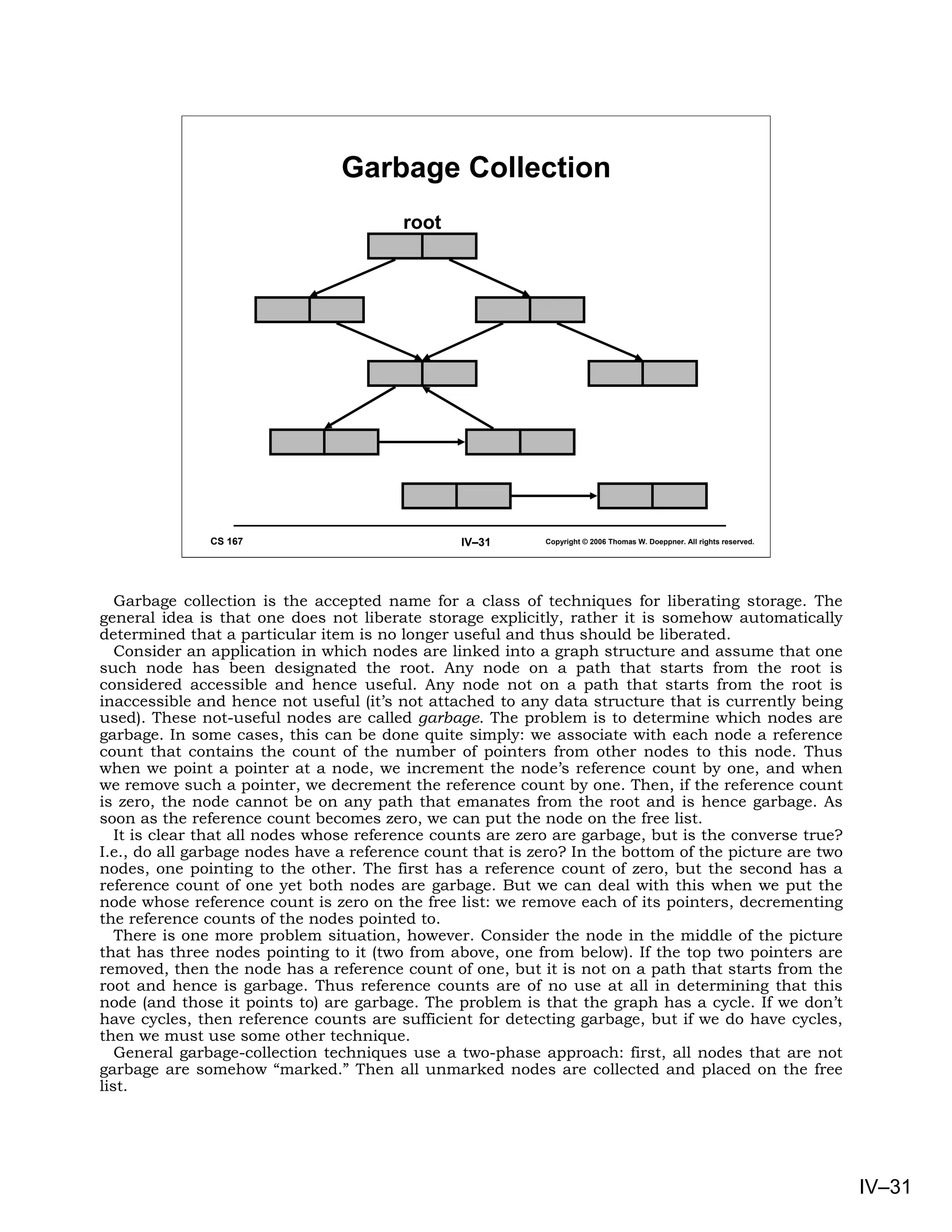
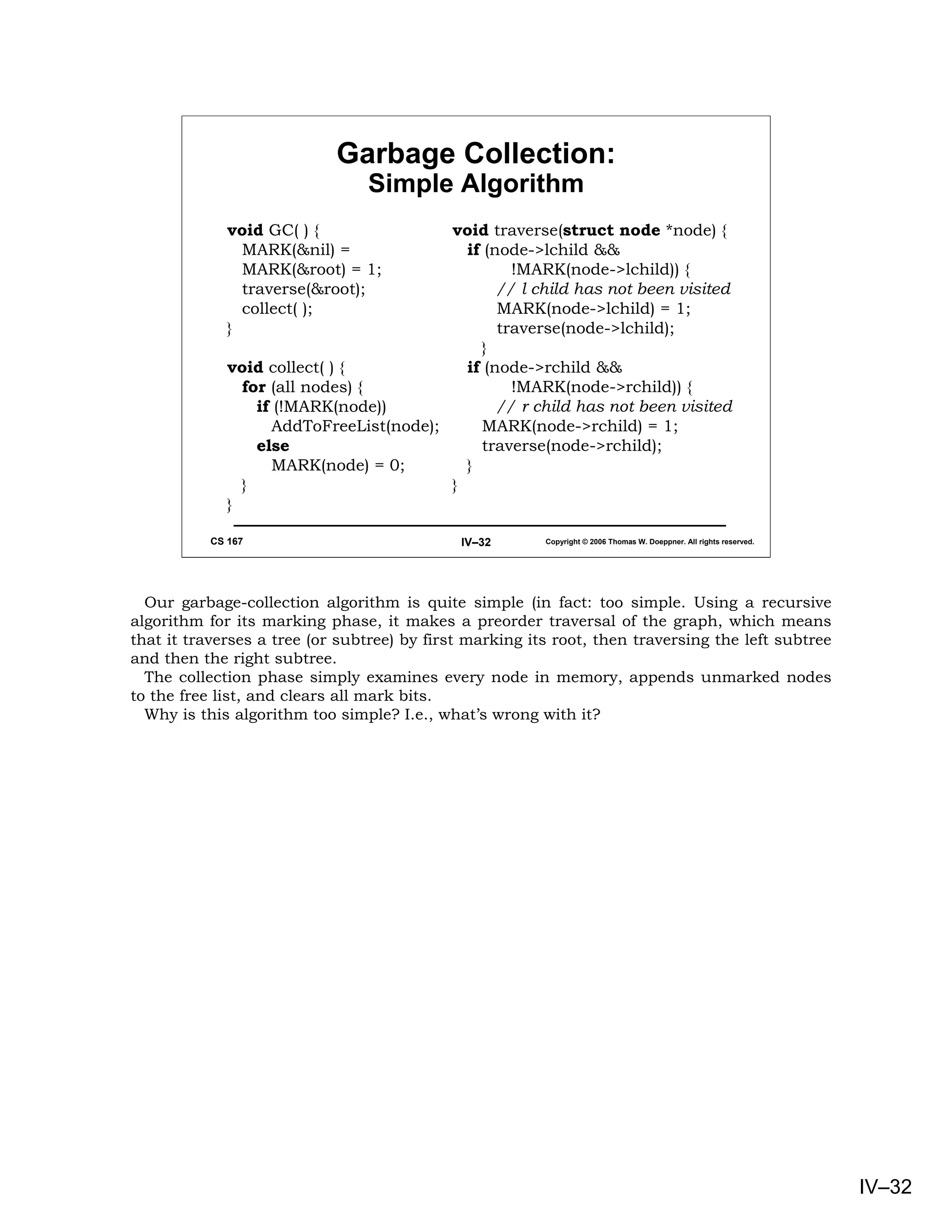
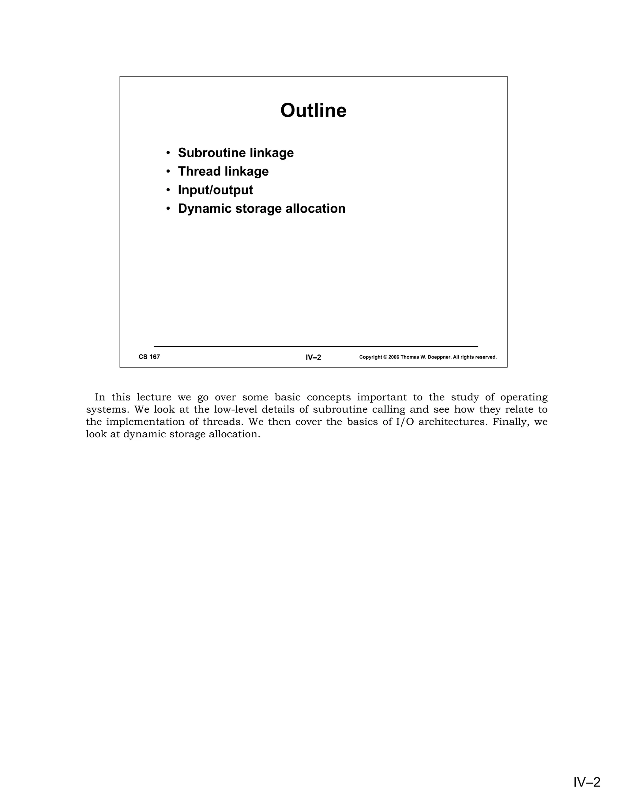
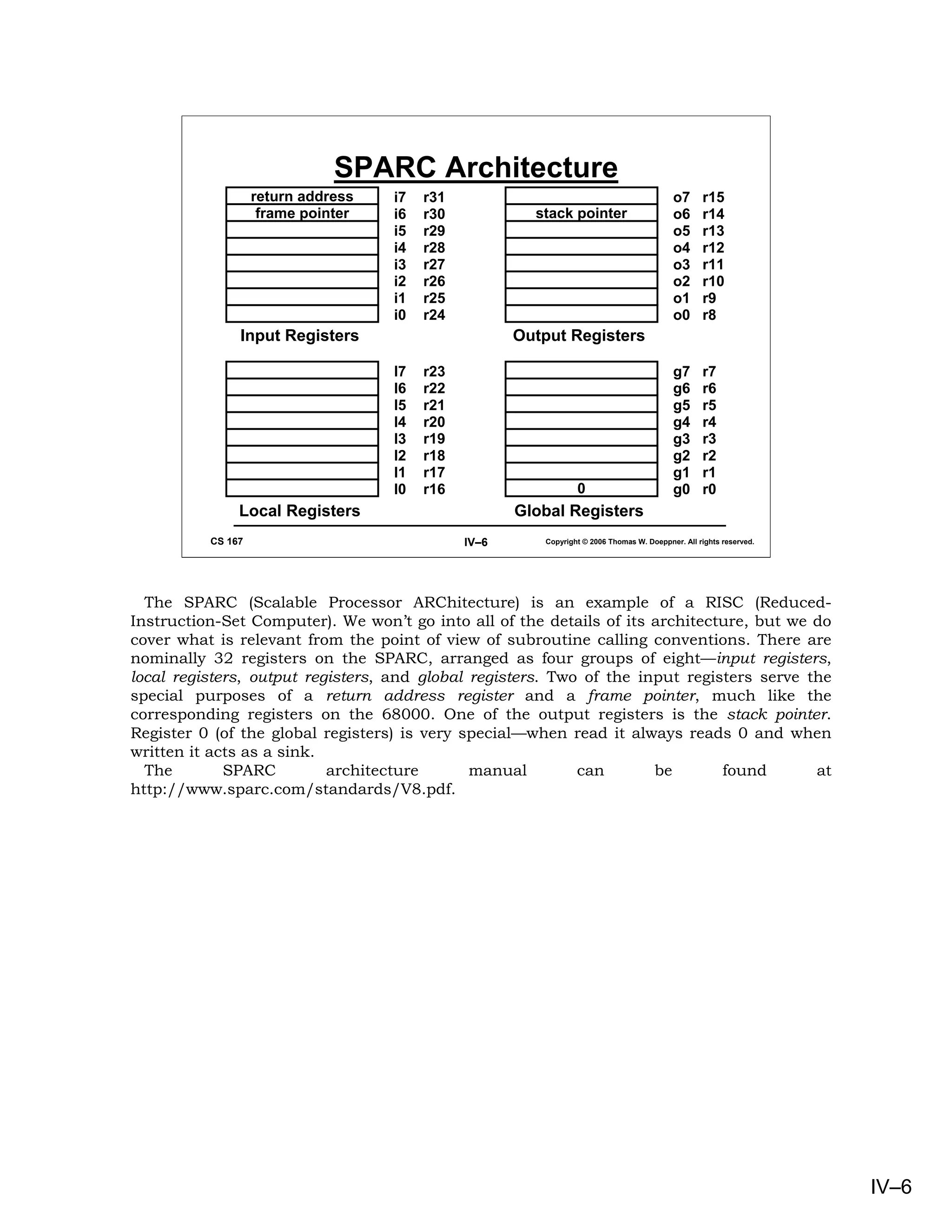
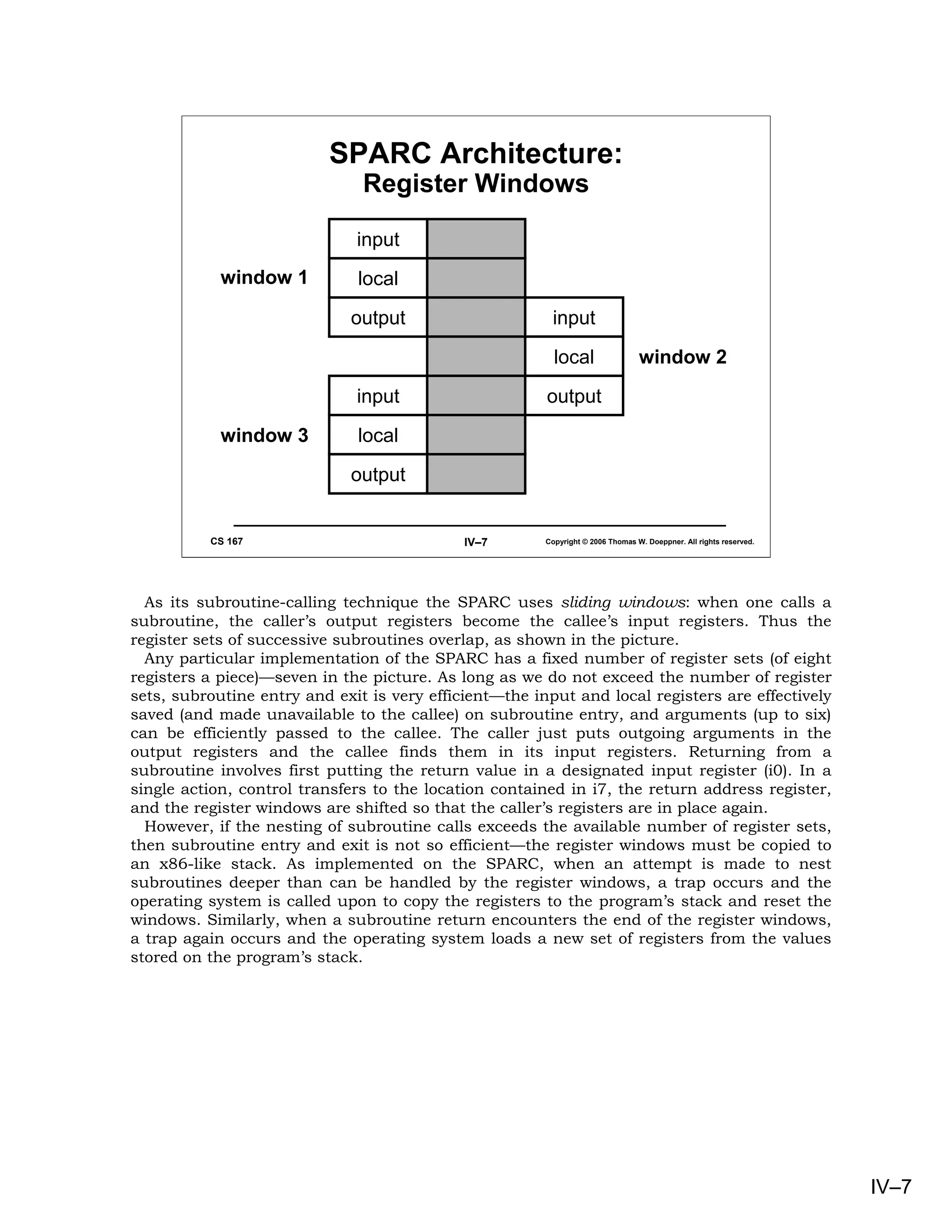
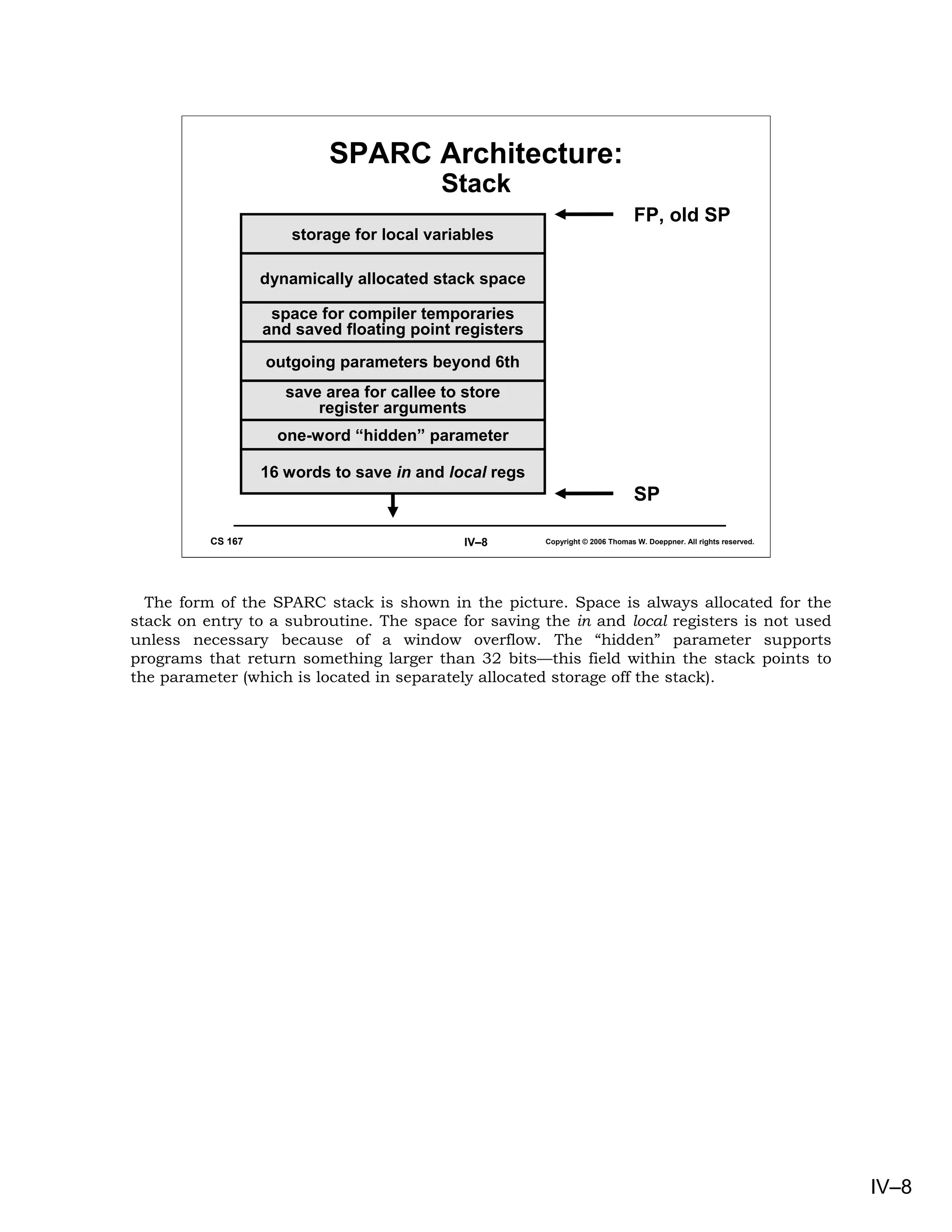
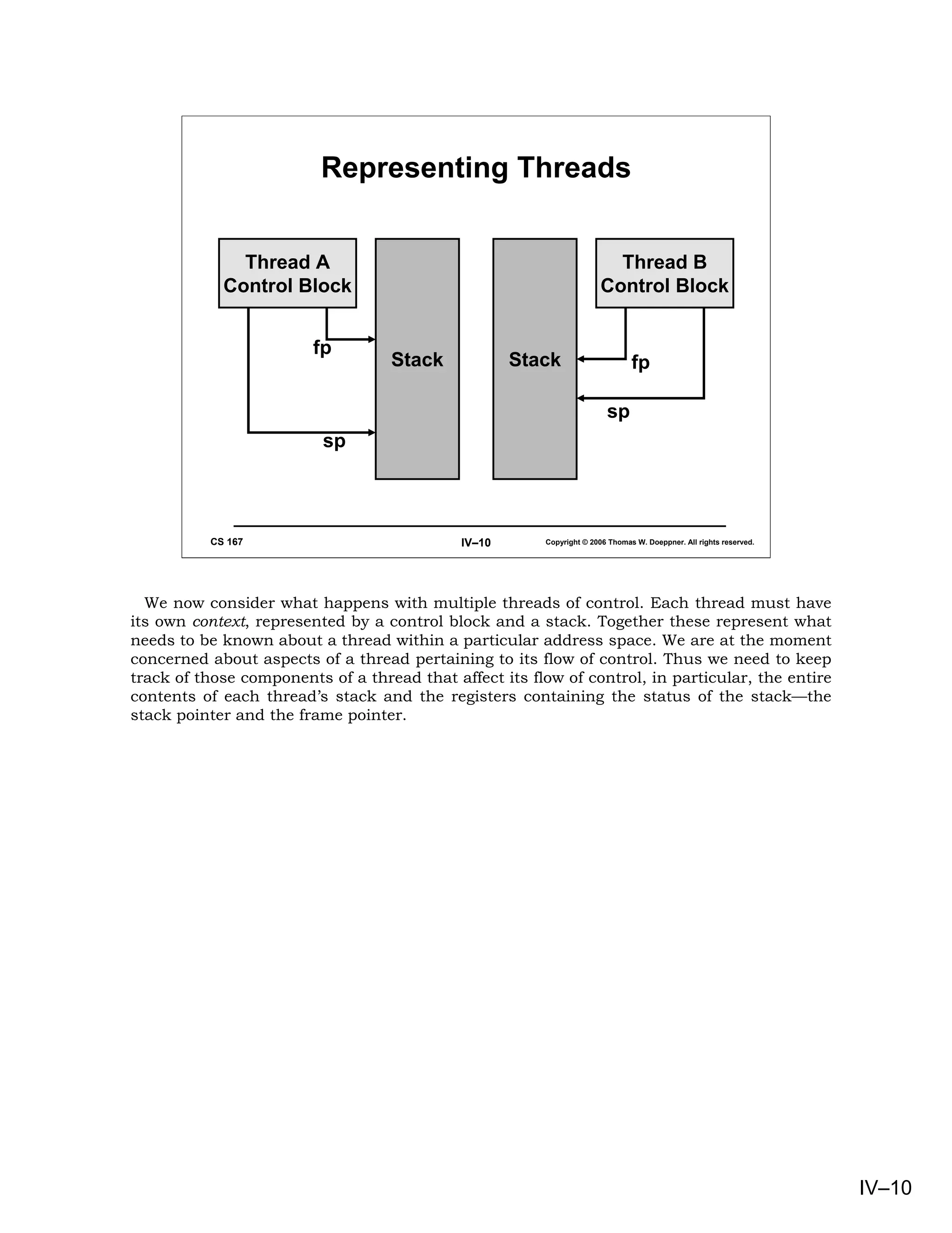
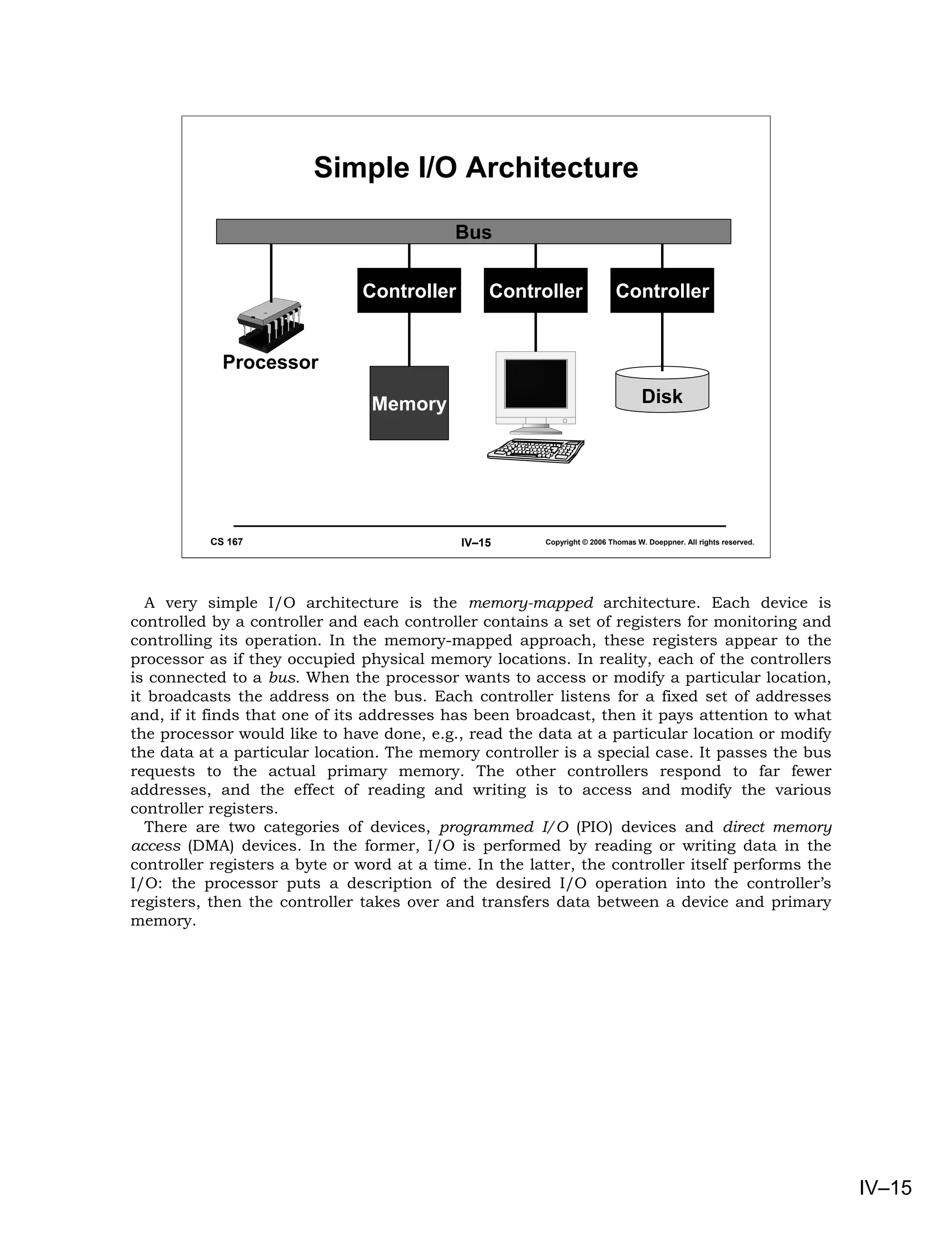
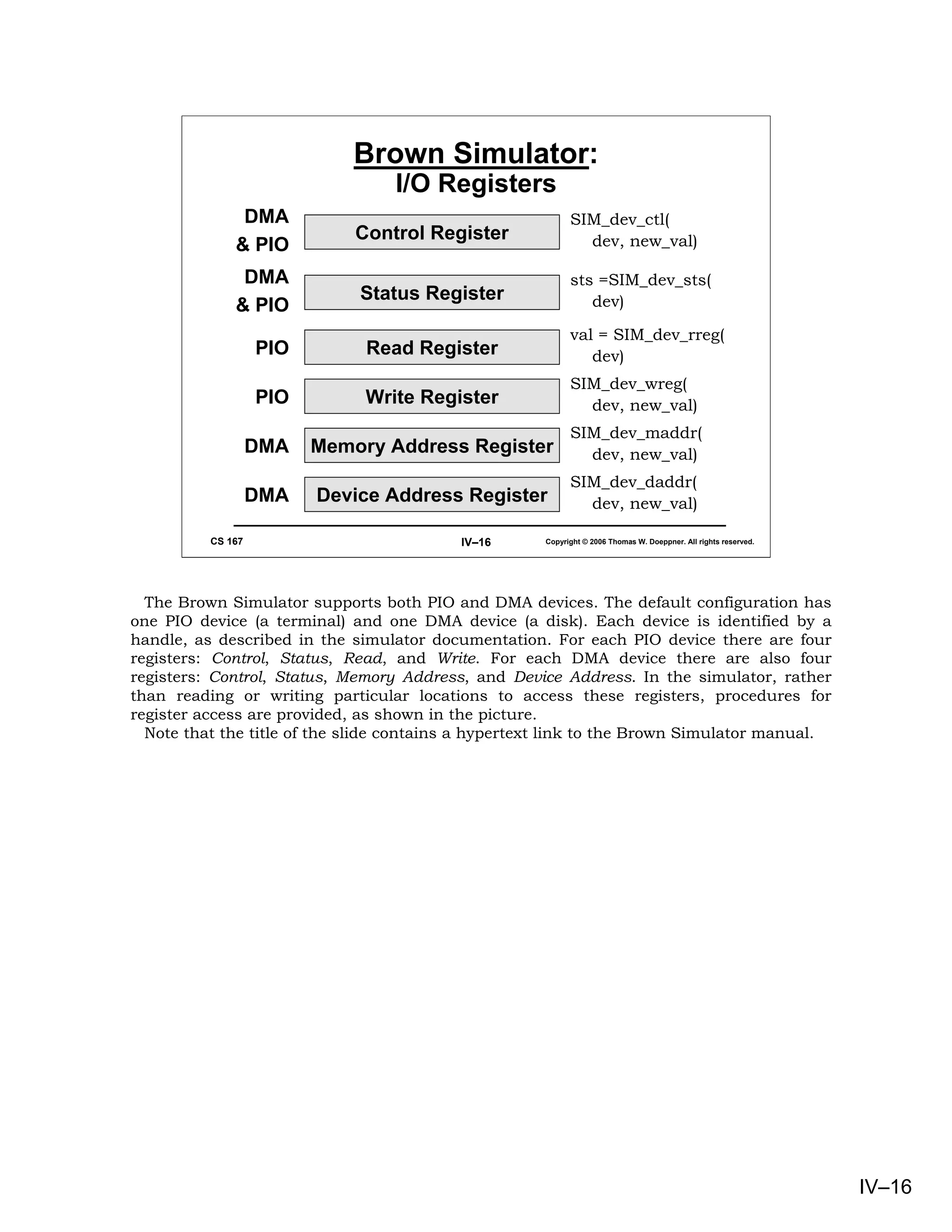
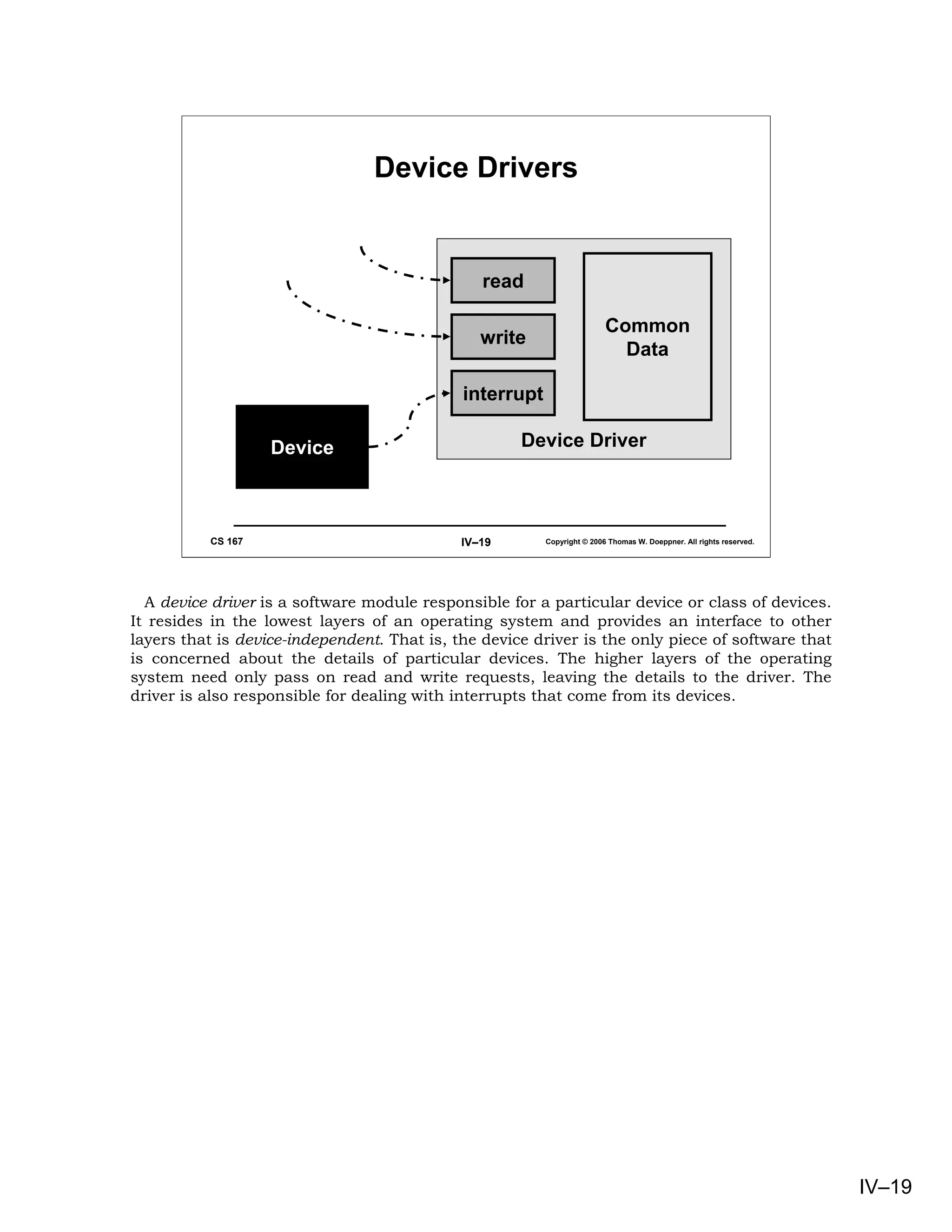
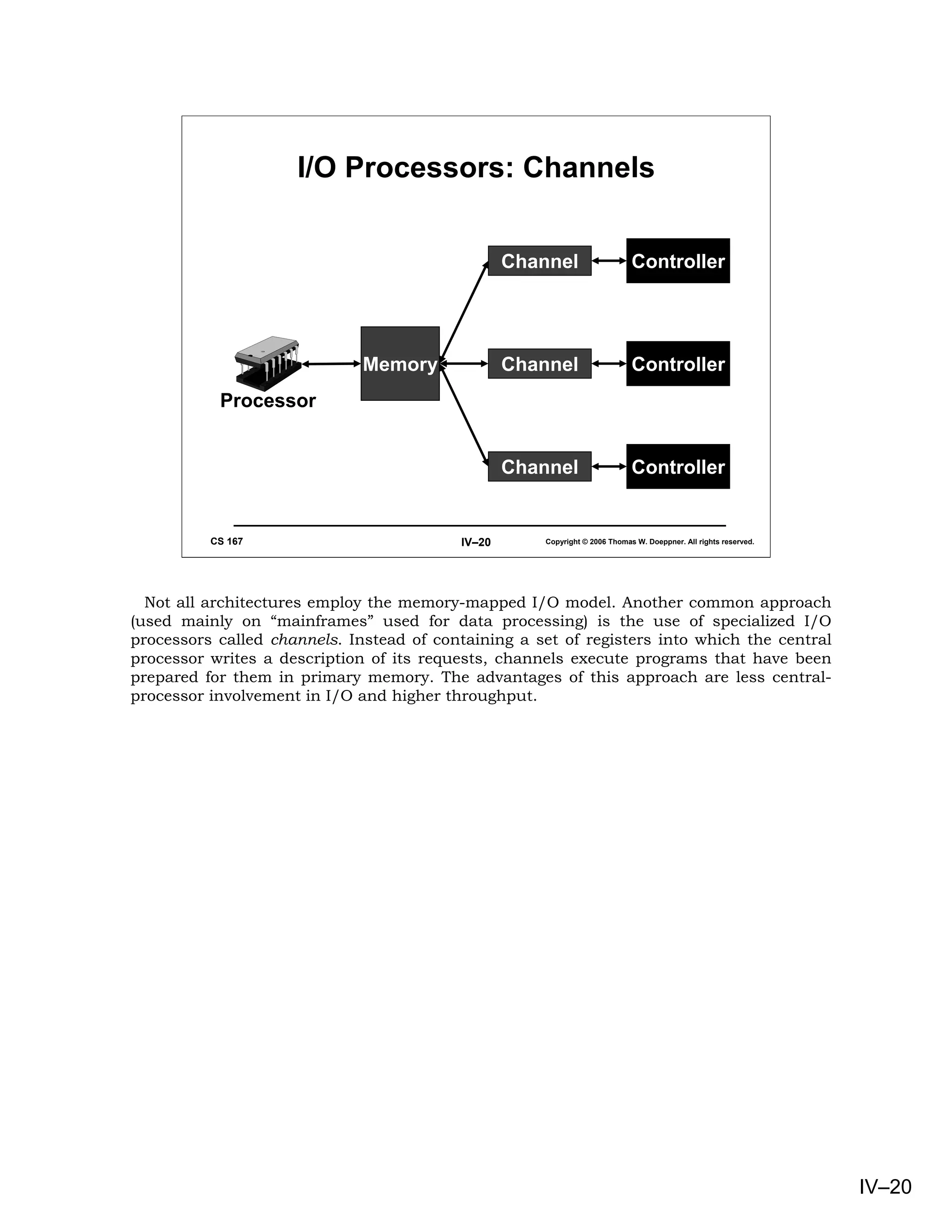
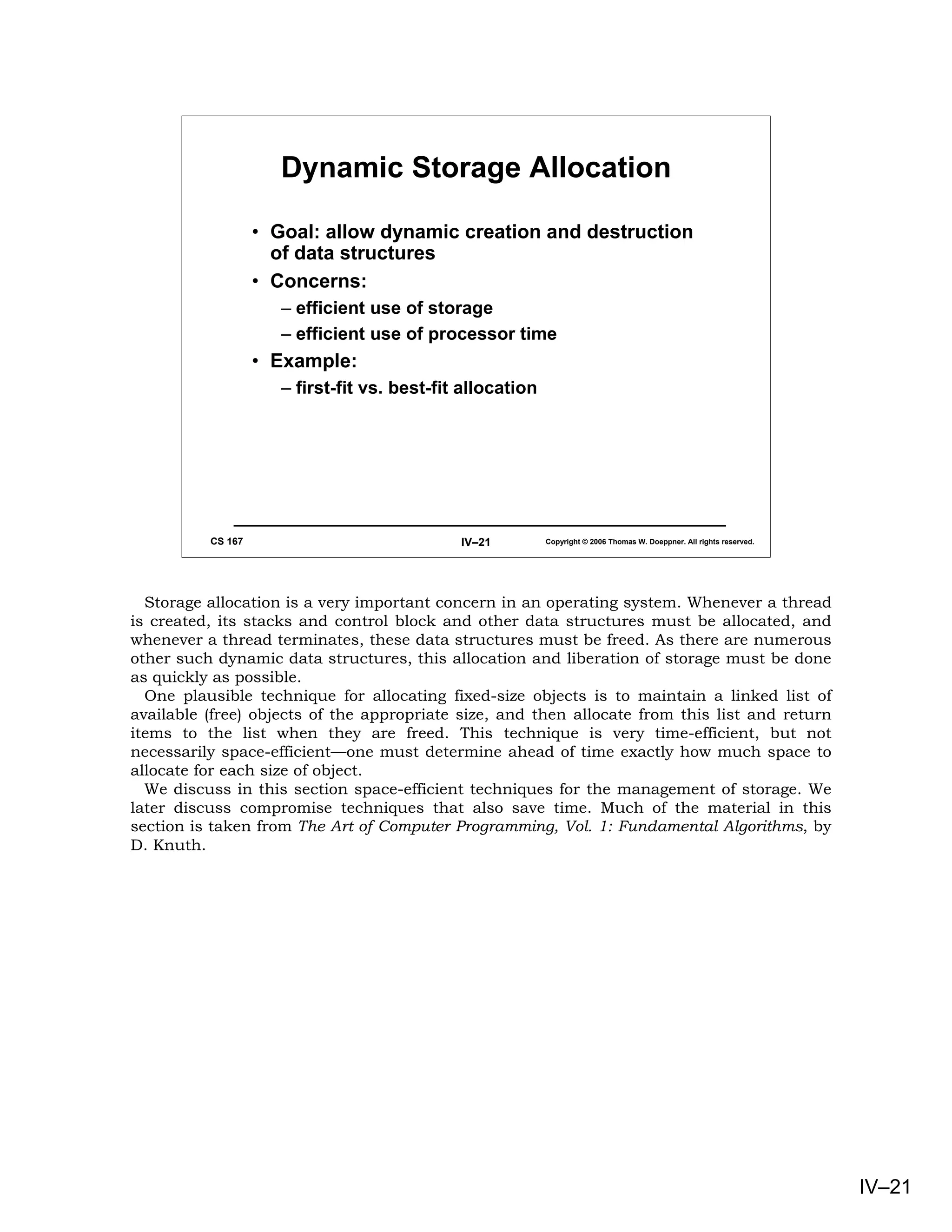
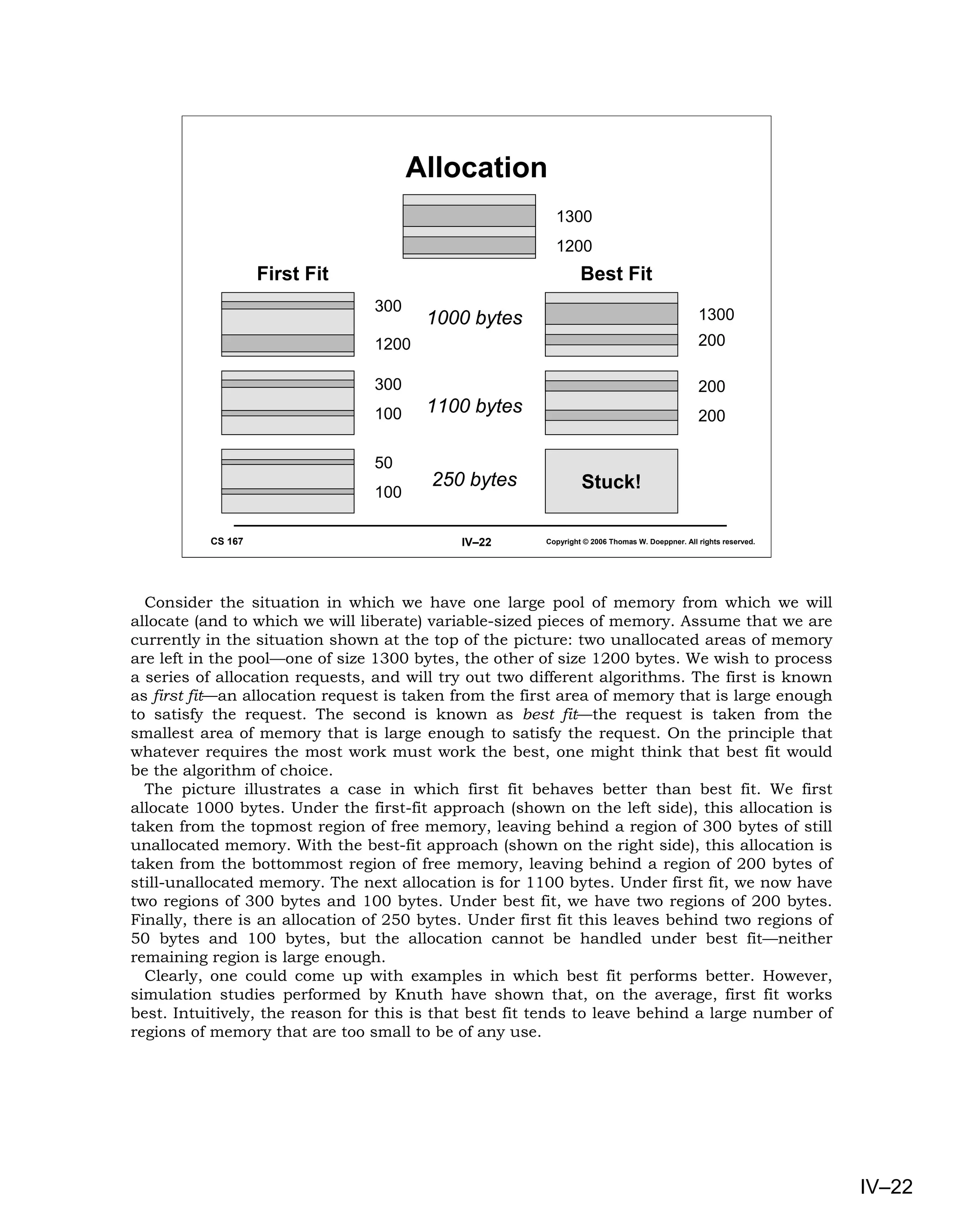
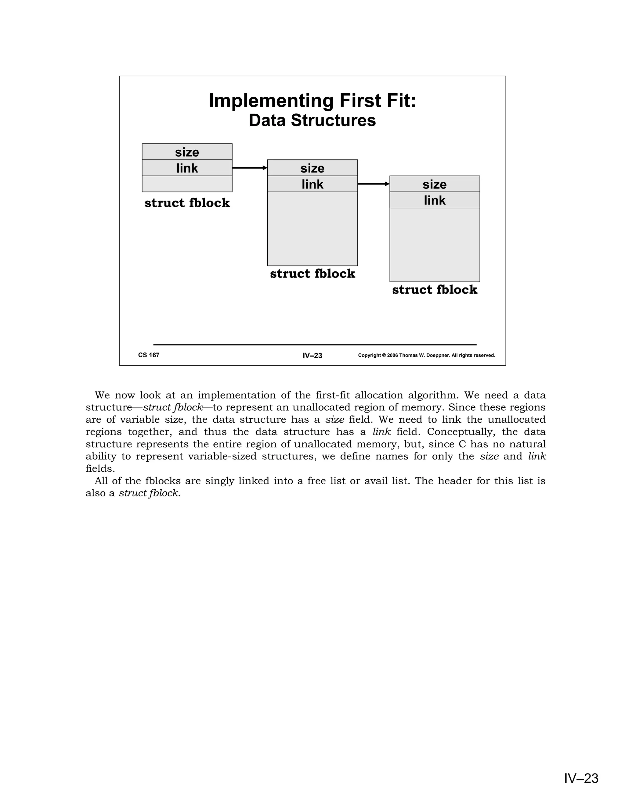
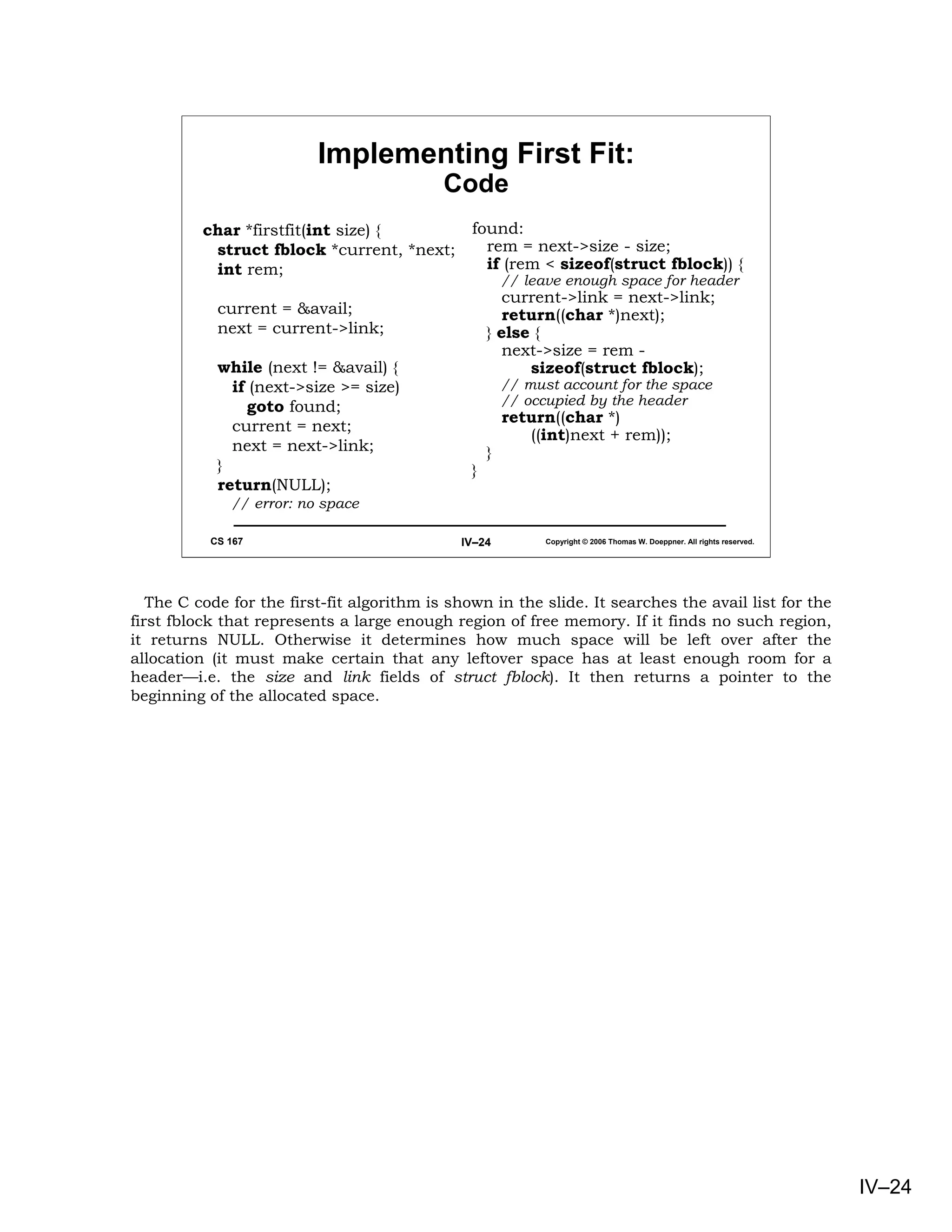
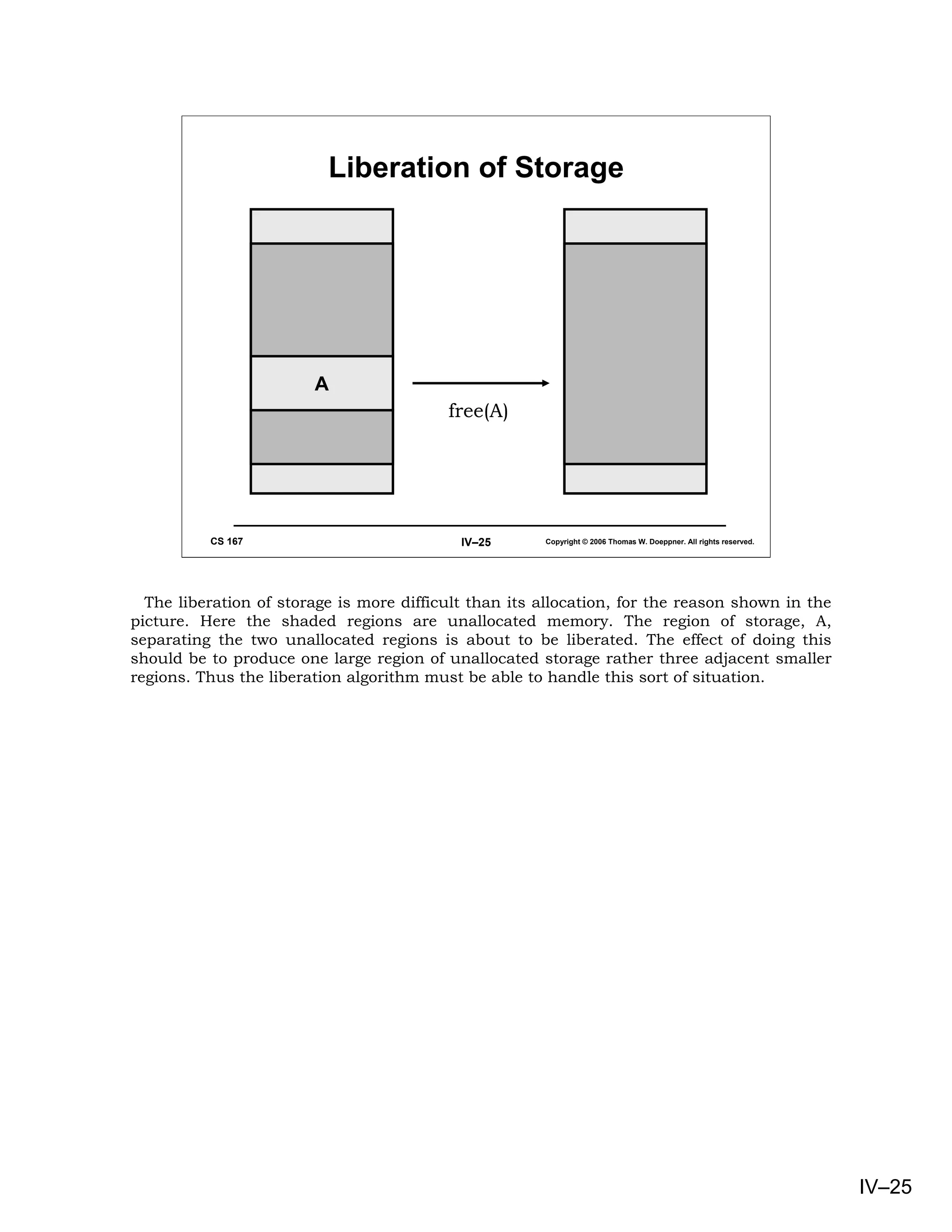
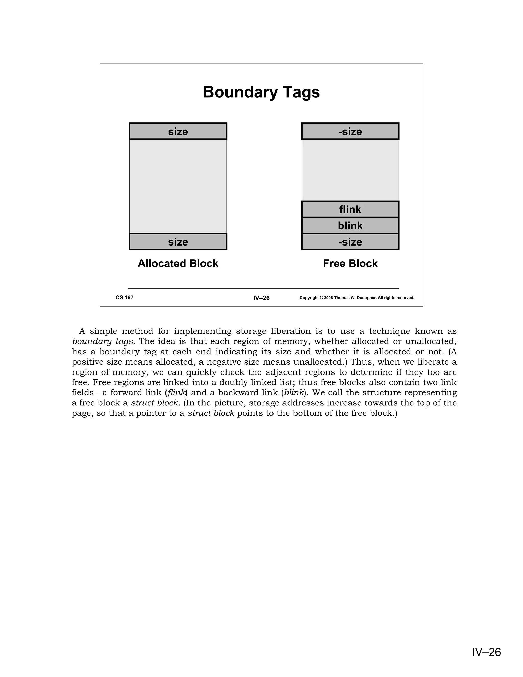
This document provides an overview of basic concepts in operating systems, including subroutine linkage, thread linkage, input/output, and dynamic storage allocation. It discusses subroutine linkage on Intel x86 and SPARC architectures, including how stack frames are used. It also covers the implementation of threads using control blocks and stacks for each thread context. Finally, it discusses input/output architectures and system calls.
![Intel x86:
Subroutine Code
_main PROC NEAR _sub PROC NEAR
push ebp ; push frame ptr push ebp ; push f ptr
mov ebp, esp ; set frame ptr mov ebp, esp ; set f ptr
sub esp, 8 ; space for locals mov eax, 8[ebp] ; get x
push 1 ; push arg 2 add eax, 12[ebp] ; add y
mov eax, -4[ebp] ; get a pop ebp ; pop f ptr
push eax ; push a ret 0 ; return
call sub
add esp, 8 ; pop args
mov -8[ebp], eax ; store in i
xor eax, eax ; return 0
mov esp, ebp ; restore stk ptr
pop ebp ; pop f ptr
ret 0 ; return
CS 167 IV–5 Copyright © 2006 Thomas W. Doeppner. All rights reserved.
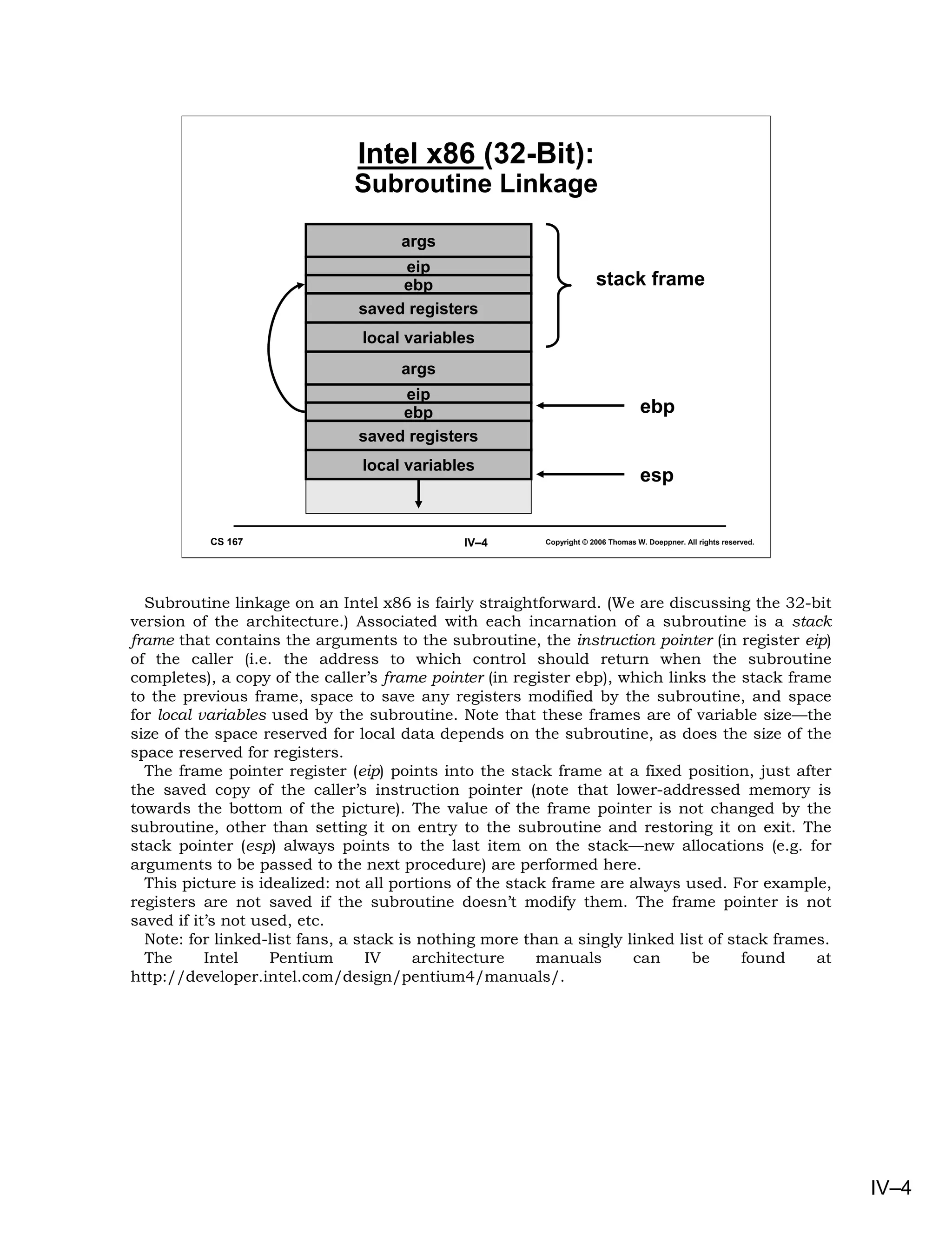
Here we see assembler code based on the win32 calling sequence produced by the
Microsoft Visual C++ compiler (with no optimization). In the main routine, first the frame
pointer is pushed on the stack (following the arguments and instruction pointer (return
address) which had been pushed by the caller). Next the current stack pointer is copied
into the frame pointer register (ebp), thereby establishing a fixed reference into the stack
frame. Space is now allocated on the stack for two local variables (occupying a total of eight
bytes) by subtracting eight from the stack pointer.
At this point the entry code for the main routine is complete and we now get ready to call
the subroutine. First the arguments are pushed onto the stack, in reverse order. Note that
a is referred to as four below the frame pointer (i.e., the first of the local variables). The
subroutine is called. On return, the two arguments are popped off the stack by adding their
size to the stack pointer. The return value of sub, in register eax, is stored into i.
Now the main routine is ready to return to its caller. It clears the return register (eax), so
as to return a zero, restores the stack pointer’s value to what was earlier copied into the
frame pointer (thereby popping the local variables from the stack), restores the frame
pointer by popping it off the stack, and finally returns to the caller.
The action in the subroutine sub is similar. First the frame pointer (ebp) is pushed onto
the stack, then the current stack pointer (esp) is copied into the frame pointer register.
With the stack frame’s location established by the frame pointer, the code accesses the two
parameters as 8 and 12 above the position pointed to by the frame pointer, respectively.
The sum of the two parameters is stored in the result register (eax), the old frame pointer is
popped from the stack, and finally an ret instruction is ececuted to pop the return address
off the stack and return to it.
IV–5](https://image.slidesharecdn.com/04basicconcepts-090825003954-phpapp01/75/04basic-Concepts-5-2048.jpg)
![SPARC Architecture:
Subroutine Code
ld [%fp-8], %o0 sub:
! put local var (a) save %sp, -64, %sp
! into out register ! push a new
mov 1, %o1 ! stack frame
add %i0, %i1, %i0
! deal with 2nd
! compute sum
! parameter ret
call sub ! return to caller
nop restore
st %o0, [%fp-4] ! pop frame off
! store result into ! stack (in delay slot)
! local var (i)
...
CS 167 IV–9 Copyright © 2006 Thomas W. Doeppner. All rights reserved.
Here we see the assembler code produced by a compiler for the SPARC. The first step, in
preparation for a subroutine call, is to put the outgoing parameters into the output
registers. The first parameter, a from our original C program, is a local variable and is
found in the stack frame. The second parameter is a constant. The call instruction merely
saves the program counter in o7 and then transfers control to the indicated address. In the
subroutine, the save instruction creates a new stack frame and advances the register
windows. It creates the new stack frame by taking the old value of the stack pointer (in the
caller’s o6), subtracting from it the amount of space that is needed (64 bytes in this
example), and storing the result into the callee’s stack pointer (o6 of the callee). At the
same time, it also advances the register windows, so that the caller’s output registers
become the callee’s input registers. If there is a window overflow, then the operating system
takes over.
Inside the subroutine, the return value is computed and stored into the callee’s i0. The
restore instruction pops the stack and backs down the register windows. Thus what the
callee left in i0 is found by the caller in o0.
IV–9](https://image.slidesharecdn.com/04basicconcepts-090825003954-phpapp01/75/04basic-Concepts-9-2048.jpg)
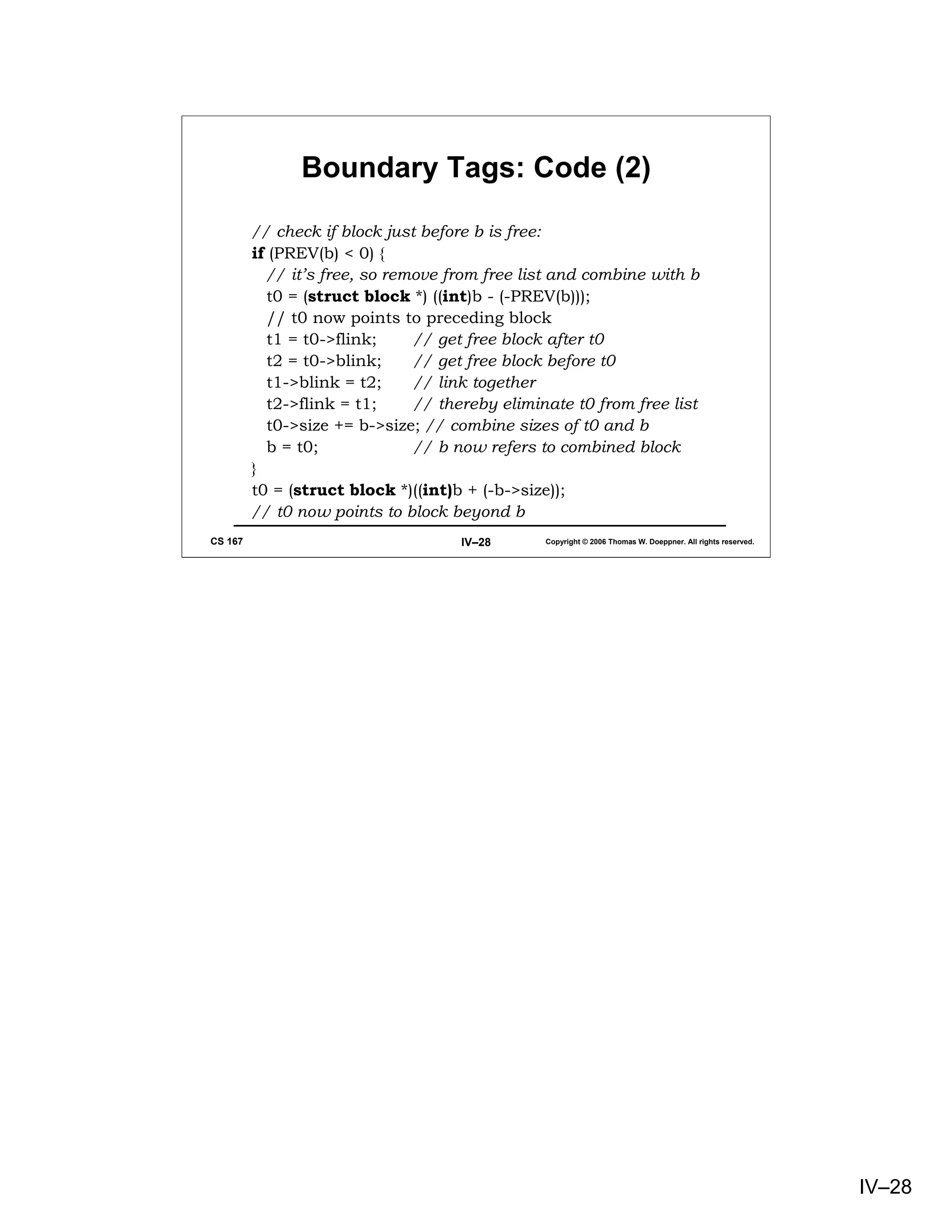
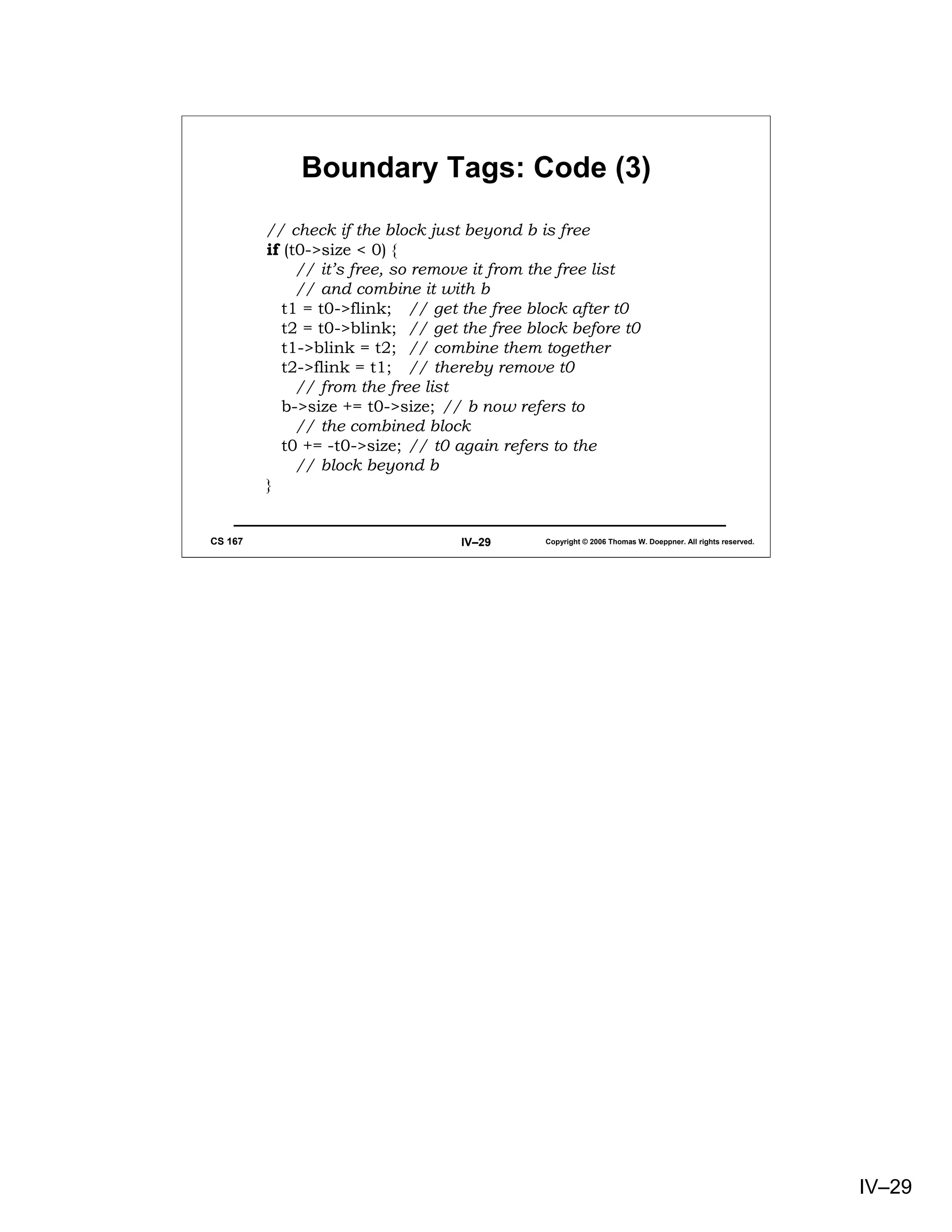
![Boundary Tags: Code (1)
#define PREV(x) (((int *)x)[-1])
struct block avail;
// assume that avail is initialized to refer
// to list of available storage
void free(struct block *b) {
struct block *t0, *t1, *t2;
b = (struct block *)&PREV(b);
// b, as provided by the caller (who is not aware of the
// tags), points to the memory just after the boundary tag
b->size = -b->size;
// adjust the tag to indicate that the storage is “free”
CS 167 IV–27 Copyright © 2006 Thomas W. Doeppner. All rights reserved.
This slide and the next presents the C code implementing liberation with boundary tags.
We define the macro PREV which, given the address of a struct block, returns the size
field of the preceding block.
The algorithm proceeds as follows. We first mark the beginning tag field of the block
being liberated to indicate that it is free. We then check to see if the previous adjacent
block is also free. If it is, we pull this block out of the free list and combine it with the block
being allocated. We then check to see if the block following the one being liberated is free. If
it is, we pull it out of the list and combine it with the block being liberated (which, of
course, may have already been combined with a previous block). Finally, after adjusting the
size fields in the tags, we insert the possibly combined block into the beginning of the free
list.
IV–27](https://image.slidesharecdn.com/04basicconcepts-090825003954-phpapp01/75/04basic-Concepts-27-2048.jpg)