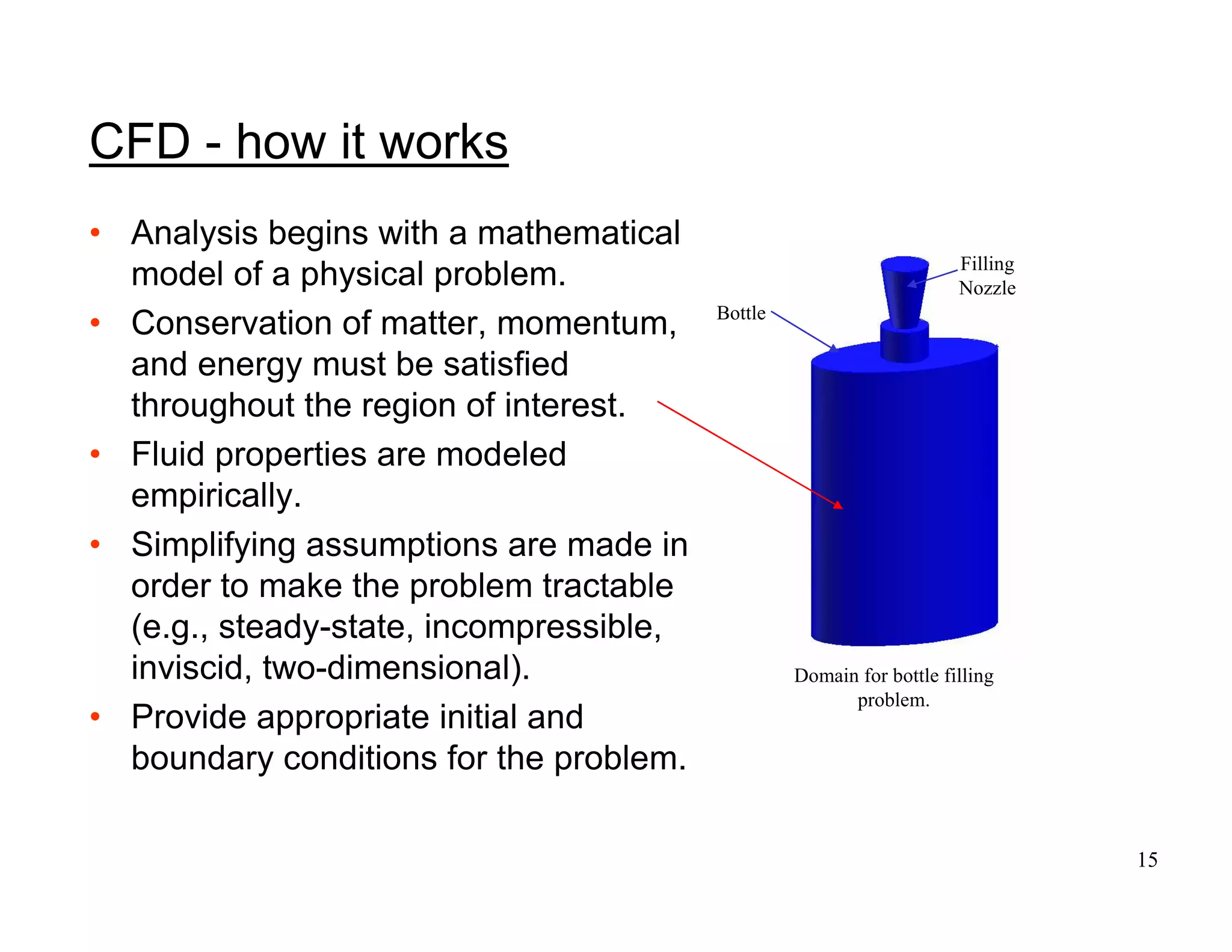
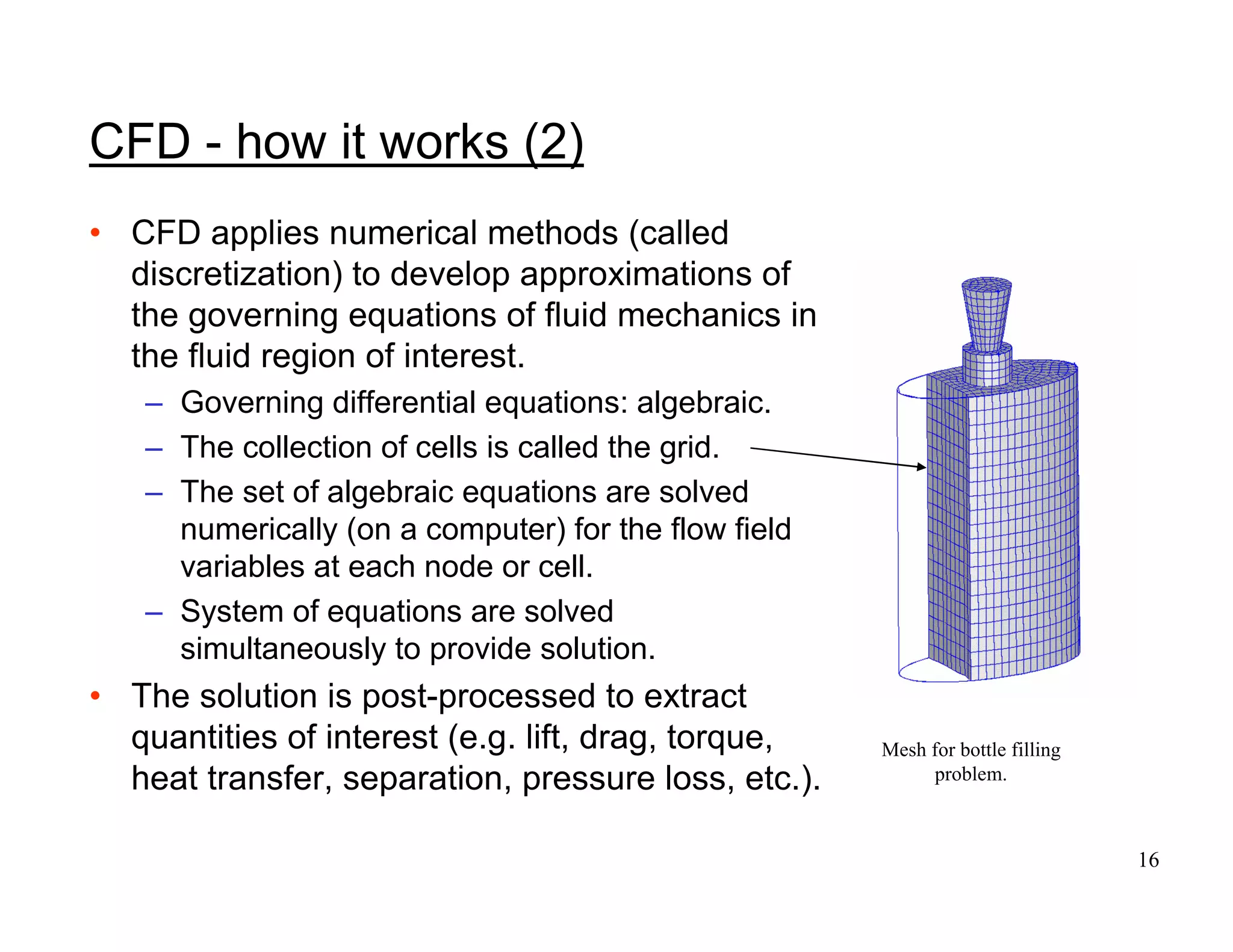
SlideShare a Scribd company logo
1
Lecture 1 - Introduction to CFD
Applied Computational Fluid Dynamics
Instructor: André Bakker
http://www.bakker.org
© André Bakker (2002-2006)
© Fluent Inc. (2002)
2
Fluid dynamics
• Fluid dynamics is the science of fluid motion.
• Fluid flow is commonly studied in one of three ways:
– Experimental fluid dynamics.
– Theoretical fluid dynamics.
– Numerically: computational fluid dynamics (CFD).
• During this course we will focus on obtaining the knowledge
required to be able to solve practical fluid flow problems using
CFD.
• Topics covered today include:
– A brief review of the history of fluid dynamics.
– An introductory overview of CFD.
3
Antiquity
• Focus on waterworks: aqueducts,
canals, harbors, bathhouses.
• One key figure was Archimedes -
Greece (287-212 BC). He initiated
the fields of static mechanics,
hydrostatics, and pycnometry (how
to measure densities and volumes of
objects).
• One of Archimedes’ inventions is the
water screw, which can be used to
lift and transport water and granular
materials.
4
Leonardo da Vinci - Italy (1452-1519)
• Leonardo set out to observe all
natural phenomena in the visible
world, recognizing their form and
structure, and describing them
pictorially exactly as they are.
• He planned and supervised canal
and harbor works over a large part
of middle Italy. In France he
designed a canal that connected the
Loire and Saone.
• His contributions to fluid mechanics
are presented in a nine part treatise
(Del moto e misura dell’acqua) that
covers the water surface, movement
of water, water waves, eddies, falling
water, free jets, interference of
waves, and many other newly
observed phenomena.
5
Leonardo da Vinci “A Gigantic Explosion”
6
Isaac Newton - England (1643-1727)
• One of the most important figures in
science.
• Most well known for his three laws of
motion.
• His key contributions to fluid mechanics
include:
– The second law: F=m.a.
– The concept of Newtonian viscosity in
which stress and the rate of strain vary
linearly.
– The reciprocity principle: the force applied
upon a stationary object by a moving fluid
is equal to the change in momentum of the
fluid as it deflects around the front of the
object.
– Relationship between the speed of waves
at a liquid surface and the wavelength.
7
• During this period, significant work was done trying to
mathematically describe the motion of fluids.
• Daniel Bernoulli (1700-1782) derived Bernoulli’s equation.
• Leonhard Euler (1707-1783) proposed the Euler equations, which
describe conservation of momentum for an inviscid fluid, and
conservation of mass. He also proposed the velocity potential
theory.
• Claude Louis Marie Henry Navier (1785-1836) and George
Gabriel Stokes (1819-1903) introduced viscous transport into the
Euler equations, which resulted in the Navier-Stokes equation.
This forms the basis of modern day CFD.
• Other key figures were Jean Le Rond d’Alembert, Siméon-Denis
Poisson, Joseph Louis Lagrange, Jean Louis Marie Poiseuille,
John William Rayleigh, M. Maurice Couette, and Pierre Simon de
Laplace.
18th and 19th century
8
Osborne Reynolds - England (1842-1912)
• Reynolds was a prolific writer who
published almost 70 papers during
his lifetime on a wide variety of
science and engineering related
topics.
• He is most well-known for the
Reynolds number, which is the ratio
between inertial and viscous forces
in a fluid. This governs the transition
from laminar to turbulent flow.
• Reynolds’ apparatus consisted of a long glass pipe through which water
could flow at different rates, controlled by a valve at the pipe exit. The
state of the flow was visualized by a streak of dye injected at the entrance
to the pipe. The flow rate was monitored by measuring the rate at which
the free surface of the tank fell during draining. The immersion of the pipe
in the tank provided temperature control due to the large thermal mass of
the fluid.
9
First part of the 20th century
• Much work was done on refining
theories of boundary layers and
turbulence.
• Ludwig Prandtl (1875-1953):
boundary layer theory, the mixing
length concept, compressible flows,
the Prandtl number, and more.
• Theodore von Karman (1881-1963)
analyzed what is now known as the
von Karman vortex street.
• Geoffrey Ingram Taylor (1886-1975):
statistical theory of turbulence and
the Taylor microscale.
• Andrey Nikolaevich Kolmogorov
(1903-1987): the Kolmogorov scales
and the universal energy spectrum.
• George Keith Batchelor (1920-2000):
contributions to the theory of
homogeneous turbulence.
10
Lewis Fry Richardson (1881-1953)
• In 1922, Lewis Fry Richardson developed the first numerical
weather prediction system.
– Division of space into grid cells and the finite difference
approximations of Bjerknes's "primitive differential equations.”
– His own attempt to calculate weather for a single eight-hour period
took six weeks and ended in failure.
• His model's enormous calculation requirements led Richardson to
propose a solution he called the “forecast-factory.”
– The "factory" would have filled a vast stadium with 64,000 people.
– Each one, armed with a mechanical calculator, would perform part of
the calculation.
– A leader in the center, using colored signal lights and telegraph
communication, would coordinate the forecast.
11
1930s to 1950s
• Earliest numerical solution: for flow past a cylinder (1933).
• A.Thom, ‘The Flow Past Circular Cylinders at Low Speeds’, Proc. Royal
Society, A141, pp. 651-666, London, 1933
• Kawaguti obtains a solution for flow around a cylinder, in 1953 by
using a mechanical desk calculator, working 20 hours per week
for 18 months, citing: “a considerable amount of labour and
endurance.”
• M. Kawaguti, ‘Numerical Solution of the NS Equations for the Flow
Around a Circular Cylinder at Reynolds Number 40’, Journal of Phy.
Soc. Japan, vol. 8, pp. 747-757, 1953.
12
1960s and 1970s
• During the 1960s the theoretical division at Los Alamos contributed many
numerical methods that are still in use today, such as the following methods:
– Particle-In-Cell (PIC).
– Marker-and-Cell (MAC).
– Vorticity-Streamfunction Methods.
– Arbitrary Lagrangian-Eulerian (ALE).
– k-ε turbulence model.
• During the 1970s a group working under D. Brian Spalding, at Imperial College,
London, develop:
– Parabolic flow codes (GENMIX).
– Vorticity-Streamfunction based codes.
– The SIMPLE algorithm and the TEACH code.
– The form of the k-ε equations that are used today.
– Upwind differencing.
– ‘Eddy break-up’ and ‘presumed pdf’ combustion models.
• In 1980 Suhas V. Patankar publishes Numerical Heat Transfer and Fluid Flow,
probably the most influential book on CFD to date.
13
1980s and 1990s
• Previously, CFD was performed using academic, research and in-
house codes. When one wanted to perform a CFD calculation,
one had to write a program.
• This is the period during which most commercial CFD codes
originated that are available today:
– Fluent (UK and US).
– CFX (UK and Canada).
– Fidap (US).
– Polyflow (Belgium).
– Phoenix (UK).
– Star CD (UK).
– Flow 3d (US).
– ESI/CFDRC (US).
– SCRYU (Japan).
– and more, see www.cfdreview.com.
14
What is computational fluid dynamics?
• Computational fluid dynamics (CFD) is the science of predicting
fluid flow, heat transfer, mass transfer, chemical reactions, and
related phenomena by solving the mathematical equations which
govern these processes using a numerical process.
• The result of CFD analyses is relevant engineering data used in:
– Conceptual studies of new designs.
– Detailed product development.
– Troubleshooting.
– Redesign.
• CFD analysis complements testing and experimentation.
– Reduces the total effort required in the laboratory.
15
Domain for bottle filling
problem.
Filling
Nozzle
Bottle
CFD - how it works
• Analysis begins with a mathematical
model of a physical problem.
• Conservation of matter, momentum,
and energy must be satisfied
throughout the region of interest.
• Fluid properties are modeled
empirically.
• Simplifying assumptions are made in
order to make the problem tractable
(e.g., steady-state, incompressible,
inviscid, two-dimensional).
• Provide appropriate initial and
boundary conditions for the problem.
16
Mesh for bottle filling
problem.
CFD - how it works (2)
• CFD applies numerical methods (called
discretization) to develop approximations of
the governing equations of fluid mechanics in
the fluid region of interest.
– Governing differential equations: algebraic.
– The collection of cells is called the grid.
– The set of algebraic equations are solved
numerically (on a computer) for the flow field
variables at each node or cell.
– System of equations are solved
simultaneously to provide solution.
• The solution is post-processed to extract
quantities of interest (e.g. lift, drag, torque,
heat transfer, separation, pressure loss, etc.).
17
Discretization
• Domain is discretized into a finite set of control volumes
or cells. The discretized domain is called the “grid” or the “mesh.”
• General conservation (transport) equations for mass, momentum,
energy, etc., are discretized into algebraic equations.
• All equations are solved to render flow field.
∫
∫
∫
∫ +
⋅
∇
Γ
=
⋅
+
∂
∂
V
A
A
V
dV
S
d
d
dV
t
φ
φ
ρφ
ρφ A
A
V
unsteady convection diffusion generation
Eqn.
continuity 1
x-mom. u
y-mom. v
energy h
φ
φ
φ
φ
Fluid region of
pipe flow
discretized into
finite set of
control volumes
(mesh).
control
volume
18
Design and create the grid
• Should you use a quad/hex grid, a tri/tet grid, a hybrid grid, or a
non-conformal grid?
• What degree of grid resolution is required in each region of the
domain?
• How many cells are required for the problem?
• Will you use adaption to add resolution?
• Do you have sufficient computer memory?
triangle
quadrilateral
tetrahedron pyramid
prism or wedge
hexahedron
arbitrary polyhedron
19
Tri/tet vs. quad/hex meshes
• For simple geometries, quad/hex
meshes can provide high-quality
solutions with fewer cells than a
comparable tri/tet mesh.
• For complex geometries,
quad/hex meshes show no
numerical advantage, and you
can save meshing effort by using
a tri/tet mesh.
20
Hybrid mesh example
• Valve port grid.
• Specific regions can be meshed
with different cell types.
• Both efficiency and accuracy are
enhanced relative to a
hexahedral or tetrahedral mesh
alone.
Hybrid mesh for an
IC engine valve port
tet mesh
hex mesh
wedge mesh
21
Dinosaur mesh example
22
Set up the numerical model
• For a given problem, you will need to:
– Select appropriate physical models.
– Turbulence, combustion, multiphase, etc.
– Define material properties.
• Fluid.
• Solid.
• Mixture.
– Prescribe operating conditions.
– Prescribe boundary conditions at all boundary zones.
– Provide an initial solution.
– Set up solver controls.
– Set up convergence monitors.
23
Compute the solution
• The discretized conservation equations are solved iteratively. A
number of iterations are usually required to reach a converged
solution.
• Convergence is reached when:
– Changes in solution variables from one iteration to the next are
negligible.
– Residuals provide a mechanism to help monitor this trend.
– Overall property conservation is achieved.
• The accuracy of a converged solution is dependent upon:
– Appropriateness and accuracy of the physical models.
– Grid resolution and independence.
– Problem setup.
24
Examine the results
• Visualization can be used to answer such questions as:
– What is the overall flow pattern?
– Is there separation?
– Where do shocks, shear layers, etc. form?
– Are key flow features being resolved?
– Are physical models and boundary conditions appropriate?
– Numerical reporting tools can be used to calculate quantitative
results, e.g:
• Lift, drag, and torque.
• Average heat transfer coefficients.
• Surface-averaged quantities.
25
Velocity vectors around a dinosaur
26
Velocity magnitude (0-6 m/s) on a dinosaur
27
Tools to examine the results
• Graphical tools:
– Grid, contour, and vector plots.
– Pathline and particle trajectory plots.
– XY plots.
– Animations.
• Numerical reporting tools:
– Flux balances.
– Surface and volume integrals and averages.
– Forces and moments.
28
Pressure field on a dinosaur
29
Forces on the dinosaur
• Drag force: 17.4 N.
• Lift force: 5.5 N.
• Wind velocity: 5 m/s.
• Air density: 1.225 kg/m3.
• The dinosaur is 3.2 m tall.
• It has a projected frontal area of A = 2.91 m2.
• The drag coefficient is:
• This is pretty good compared to the average car! The streamlined
back of the dinosaur resulted in a flow pattern with very little
separation.
11
.
0
91
.
2
*
25
*
225
.
1
*
5
.
0
4
.
17
2
2
1
=
=
=
A
v
F
C D
D
ρ
30
Consider revisions to the model
• Are physical models appropriate?
– Is flow turbulent?
– Is flow unsteady?
– Are there compressibility effects?
– Are there 3D effects?
– Are boundary conditions correct?
• Is the computational domain large enough?
– Are boundary conditions appropriate?
– Are boundary values reasonable?
• Is grid adequate?
– Can grid be adapted to improve results?
– Does solution change significantly with adaption, or is the solution
grid independent?
– Does boundary resolution need to be improved?
31
Applications of CFD
• Applications of CFD are numerous!
– Flow and heat transfer in industrial processes (boilers, heat
exchangers, combustion equipment, pumps, blowers, piping, etc.).
– Aerodynamics of ground vehicles, aircraft, missiles.
– Film coating, thermoforming in material processing applications.
– Flow and heat transfer in propulsion and power generation systems.
– Ventilation, heating, and cooling flows in buildings.
– Chemical vapor deposition (CVD) for integrated circuit
manufacturing.
– Heat transfer for electronics packaging applications.
– And many, many more!
32
Advantages of CFD
• Relatively low cost.
– Using physical experiments and tests to get essential engineering
data for design can be expensive.
– CFD simulations are relatively inexpensive, and costs are likely to
decrease as computers become more powerful.
• Speed.
– CFD simulations can be executed in a short period of time.
– Quick turnaround means engineering data can be introduced early in
the design process.
• Ability to simulate real conditions.
– Many flow and heat transfer processes can not be (easily) tested,
e.g. hypersonic flow.
– CFD provides the ability to theoretically simulate any physical
condition.
33
Advantages of CFD (2)
• Ability to simulate ideal conditions.
– CFD allows great control over the physical process, and provides the
ability to isolate specific phenomena for study.
– Example: a heat transfer process can be idealized with adiabatic,
constant heat flux, or constant temperature boundaries.
• Comprehensive information.
– Experiments only permit data to be extracted at a limited number of
locations in the system (e.g. pressure and temperature probes, heat
flux gauges, LDV, etc.).
– CFD allows the analyst to examine a large number of locations in the
region of interest, and yields a comprehensive set of flow parameters
for examination.
34
Limitations of CFD
• Physical models.
– CFD solutions rely upon physical models of real world processes
(e.g. turbulence, compressibility, chemistry, multiphase flow, etc.).
– The CFD solutions can only be as accurate as the physical models
on which they are based.
• Numerical errors.
– Solving equations on a computer invariably introduces numerical
errors.
– Round-off error: due to finite word size available on the computer.
Round-off errors will always exist (though they can be small in most
cases).
– Truncation error: due to approximations in the numerical models.
Truncation errors will go to zero as the grid is refined. Mesh
refinement is one way to deal with truncation error.
35
poor better
Fully Developed Inlet
Profile
Computational
Domain
Computational
Domain
Uniform Inlet
Profile
Limitations of CFD (2)
• Boundary conditions.
– As with physical models, the accuracy of the CFD solution is only as
good as the initial/boundary conditions provided to the numerical
model.
– Example: flow in a duct with sudden expansion. If flow is supplied to
domain by a pipe, you should use a fully-developed profile for
velocity rather than assume uniform conditions.
36
Summary
• CFD is a method to numerically calculate heat transfer and fluid
flow.
• Currently, its main application is as an engineering method, to
provide data that is complementary to theoretical and
experimental data. This is mainly the domain of commercially
available codes and in-house codes at large companies.
• CFD can also be used for purely scientific studies, e.g. into the
fundamentals of turbulence. This is more common in academic
institutions and government research laboratories. Codes are
usually developed to specifically study a certain problem.

More Related Content

Similar to 01-intro_Bakker.pdf

100-423-1-PB.pdf
100-423-1-PB.pdf100-423-1-PB.pdf
100-423-1-PB.pdf
AnimeshKumar787928
 
Mid Term Presentation.pptx
Mid Term Presentation.pptxMid Term Presentation.pptx
Mid Term Presentation.pptx
AyushYadav664474
 
A short history of hydraulics
A short history of hydraulicsA short history of hydraulics
A short history of hydraulics
BENYOUCEF Slimane
 
WHAT IS COMPUTATIONAL FLUID DYNAMICS (CFD)
WHAT IS COMPUTATIONAL FLUID DYNAMICS (CFD)WHAT IS COMPUTATIONAL FLUID DYNAMICS (CFD)
WHAT IS COMPUTATIONAL FLUID DYNAMICS (CFD)
Malik Abdul Wahab
 
Thermal Energy on Water and Oil placed Squeezed Carreau Nanofluids Flow
Thermal Energy on Water and Oil placed Squeezed Carreau Nanofluids FlowThermal Energy on Water and Oil placed Squeezed Carreau Nanofluids Flow
Thermal Energy on Water and Oil placed Squeezed Carreau Nanofluids Flow
MOHAMMED FAYYADH
 
Chapter 4 Climate change model.pptx
Chapter 4 Climate change model.pptxChapter 4 Climate change model.pptx
Chapter 4 Climate change model.pptx
AManiMaran1
 
ISOPE2021_elSheshtawy.pptx
ISOPE2021_elSheshtawy.pptxISOPE2021_elSheshtawy.pptx
ISOPE2021_elSheshtawy.pptx
HasanAdel5
 
Numerical Analysis of heat transfer in a channel Wit in clined baffles
Numerical Analysis of heat transfer in a channel Wit in clined bafflesNumerical Analysis of heat transfer in a channel Wit in clined baffles
Numerical Analysis of heat transfer in a channel Wit in clined baffles
inventy
 
IRJET-To Investigate the effect of Spinner Geometry on COP of Vortex Tube Ref...
IRJET-To Investigate the effect of Spinner Geometry on COP of Vortex Tube Ref...IRJET-To Investigate the effect of Spinner Geometry on COP of Vortex Tube Ref...
IRJET-To Investigate the effect of Spinner Geometry on COP of Vortex Tube Ref...
IRJET Journal
 
The New Engineering by Mr. Eugene F. Adiutori
The New Engineering by Mr. Eugene F. AdiutoriThe New Engineering by Mr. Eugene F. Adiutori
The New Engineering by Mr. Eugene F. Adiutori
Julio Banks
 
SMART Seminar Series: "The Evolution of the Metric System: From Precious Lump...
SMART Seminar Series: "The Evolution of the Metric System: From Precious Lump...SMART Seminar Series: "The Evolution of the Metric System: From Precious Lump...
SMART Seminar Series: "The Evolution of the Metric System: From Precious Lump...
SMART Infrastructure Facility
 
Cfd 0
Cfd 0Cfd 0
Q1232116146
Q1232116146Q1232116146
Q1232116146
IOSR Journals
 
The korteweg dvries equation a survey of results
The korteweg dvries equation a survey of resultsThe korteweg dvries equation a survey of results
The korteweg dvries equation a survey of results
Haziqah Hussin
 
HYDRAULICENGINEERING_BSCE1B.pptx
HYDRAULICENGINEERING_BSCE1B.pptxHYDRAULICENGINEERING_BSCE1B.pptx
HYDRAULICENGINEERING_BSCE1B.pptx
RazelMaeLayson
 
Lectures on Heat Transfer - Introduction - Applications - Fundamentals - Gove...
Lectures on Heat Transfer - Introduction - Applications - Fundamentals - Gove...Lectures on Heat Transfer - Introduction - Applications - Fundamentals - Gove...
Lectures on Heat Transfer - Introduction - Applications - Fundamentals - Gove...
tmuliya
 
Hr2413591363
Hr2413591363Hr2413591363
Hr2413591363
IJERA Editor
 
Effect of Radiation on Mixed Convection Flow of a Non-Newtonian Nan fluid ove...
Effect of Radiation on Mixed Convection Flow of a Non-Newtonian Nan fluid ove...Effect of Radiation on Mixed Convection Flow of a Non-Newtonian Nan fluid ove...
Effect of Radiation on Mixed Convection Flow of a Non-Newtonian Nan fluid ove...
IJMER
 

Similar to 01-intro_Bakker.pdf (20)

100-423-1-PB.pdf
100-423-1-PB.pdf100-423-1-PB.pdf
100-423-1-PB.pdf
 
Mid Term Presentation.pptx
Mid Term Presentation.pptxMid Term Presentation.pptx
Mid Term Presentation.pptx
 
10 rans
10 rans10 rans
10 rans
 
A short history of hydraulics
A short history of hydraulicsA short history of hydraulics
A short history of hydraulics
 
WHAT IS COMPUTATIONAL FLUID DYNAMICS (CFD)
WHAT IS COMPUTATIONAL FLUID DYNAMICS (CFD)WHAT IS COMPUTATIONAL FLUID DYNAMICS (CFD)
WHAT IS COMPUTATIONAL FLUID DYNAMICS (CFD)
 
Thermal Energy on Water and Oil placed Squeezed Carreau Nanofluids Flow
Thermal Energy on Water and Oil placed Squeezed Carreau Nanofluids FlowThermal Energy on Water and Oil placed Squeezed Carreau Nanofluids Flow
Thermal Energy on Water and Oil placed Squeezed Carreau Nanofluids Flow
 
Chapter 4 Climate change model.pptx
Chapter 4 Climate change model.pptxChapter 4 Climate change model.pptx
Chapter 4 Climate change model.pptx
 
ISOPE2021_elSheshtawy.pptx
ISOPE2021_elSheshtawy.pptxISOPE2021_elSheshtawy.pptx
ISOPE2021_elSheshtawy.pptx
 
Numerical Analysis of heat transfer in a channel Wit in clined baffles
Numerical Analysis of heat transfer in a channel Wit in clined bafflesNumerical Analysis of heat transfer in a channel Wit in clined baffles
Numerical Analysis of heat transfer in a channel Wit in clined baffles
 
IRJET-To Investigate the effect of Spinner Geometry on COP of Vortex Tube Ref...
IRJET-To Investigate the effect of Spinner Geometry on COP of Vortex Tube Ref...IRJET-To Investigate the effect of Spinner Geometry on COP of Vortex Tube Ref...
IRJET-To Investigate the effect of Spinner Geometry on COP of Vortex Tube Ref...
 
The New Engineering by Mr. Eugene F. Adiutori
The New Engineering by Mr. Eugene F. AdiutoriThe New Engineering by Mr. Eugene F. Adiutori
The New Engineering by Mr. Eugene F. Adiutori
 
IJHMT_2016
IJHMT_2016IJHMT_2016
IJHMT_2016
 
SMART Seminar Series: "The Evolution of the Metric System: From Precious Lump...
SMART Seminar Series: "The Evolution of the Metric System: From Precious Lump...SMART Seminar Series: "The Evolution of the Metric System: From Precious Lump...
SMART Seminar Series: "The Evolution of the Metric System: From Precious Lump...
 
Cfd 0
Cfd 0Cfd 0
Cfd 0
 
Q1232116146
Q1232116146Q1232116146
Q1232116146
 
The korteweg dvries equation a survey of results
The korteweg dvries equation a survey of resultsThe korteweg dvries equation a survey of results
The korteweg dvries equation a survey of results
 
HYDRAULICENGINEERING_BSCE1B.pptx
HYDRAULICENGINEERING_BSCE1B.pptxHYDRAULICENGINEERING_BSCE1B.pptx
HYDRAULICENGINEERING_BSCE1B.pptx
 
Lectures on Heat Transfer - Introduction - Applications - Fundamentals - Gove...
Lectures on Heat Transfer - Introduction - Applications - Fundamentals - Gove...Lectures on Heat Transfer - Introduction - Applications - Fundamentals - Gove...
Lectures on Heat Transfer - Introduction - Applications - Fundamentals - Gove...
 
Hr2413591363
Hr2413591363Hr2413591363
Hr2413591363
 
Effect of Radiation on Mixed Convection Flow of a Non-Newtonian Nan fluid ove...
Effect of Radiation on Mixed Convection Flow of a Non-Newtonian Nan fluid ove...Effect of Radiation on Mixed Convection Flow of a Non-Newtonian Nan fluid ove...
Effect of Radiation on Mixed Convection Flow of a Non-Newtonian Nan fluid ove...
 

More from ssusercf6d0e

Paul J. Boudreaux Consider a Mixed Analog/Digital/MEMs
Paul J. Boudreaux Consider a Mixed Analog/Digital/MEMsPaul J. Boudreaux Consider a Mixed Analog/Digital/MEMs
Paul J. Boudreaux Consider a Mixed Analog/Digital/MEMs
ssusercf6d0e
 
13055193.ppt This is heat sink material.
13055193.ppt This is heat sink material.13055193.ppt This is heat sink material.
13055193.ppt This is heat sink material.
ssusercf6d0e
 
Billetdefects-Off-cornercracksformationpreventionandevolution.pdf
Billetdefects-Off-cornercracksformationpreventionandevolution.pdfBilletdefects-Off-cornercracksformationpreventionandevolution.pdf
Billetdefects-Off-cornercracksformationpreventionandevolution.pdf
ssusercf6d0e
 
A_Simulation_Method_for_the_Optimization_of_Coolin-Good.pdf
A_Simulation_Method_for_the_Optimization_of_Coolin-Good.pdfA_Simulation_Method_for_the_Optimization_of_Coolin-Good.pdf
A_Simulation_Method_for_the_Optimization_of_Coolin-Good.pdf
ssusercf6d0e
 
aiaa-2000 numerical investigation premixed combustion
aiaa-2000 numerical investigation premixed combustionaiaa-2000 numerical investigation premixed combustion
aiaa-2000 numerical investigation premixed combustion
ssusercf6d0e
 
tses_article147 mathematical modeling combustion
tses_article147 mathematical modeling combustiontses_article147 mathematical modeling combustion
tses_article147 mathematical modeling combustion
ssusercf6d0e
 
detonation using cfd code 944-1-5119-1-10-20180129.pdf
detonation using cfd code 944-1-5119-1-10-20180129.pdfdetonation using cfd code 944-1-5119-1-10-20180129.pdf
detonation using cfd code 944-1-5119-1-10-20180129.pdf
ssusercf6d0e
 
How_to_blockMesh using OpenFOAM good mateiral
How_to_blockMesh using OpenFOAM good mateiralHow_to_blockMesh using OpenFOAM good mateiral
How_to_blockMesh using OpenFOAM good mateiral
ssusercf6d0e
 
complex mesh generation with openFOAM thchnical
complex mesh generation with openFOAM thchnicalcomplex mesh generation with openFOAM thchnical
complex mesh generation with openFOAM thchnical
ssusercf6d0e
 
design optimization of a single-strand tundish based on CFD
design optimization of a single-strand tundish based on CFDdesign optimization of a single-strand tundish based on CFD
design optimization of a single-strand tundish based on CFD
ssusercf6d0e
 
Numerical calculation of rotating detonation chambe
Numerical calculation of rotating detonation chambeNumerical calculation of rotating detonation chambe
Numerical calculation of rotating detonation chambe
ssusercf6d0e
 
Numerical Simulations of hot jet detonation
Numerical Simulations of hot jet detonationNumerical Simulations of hot jet detonation
Numerical Simulations of hot jet detonation
ssusercf6d0e
 
Chapter 3.pdf
Chapter 3.pdfChapter 3.pdf
Chapter 3.pdf
ssusercf6d0e
 
Chapter_5.pdf
Chapter_5.pdfChapter_5.pdf
Chapter_5.pdf
ssusercf6d0e
 
Chapter 6.pdf
Chapter 6.pdfChapter 6.pdf
Chapter 6.pdf
ssusercf6d0e
 
CFD_Lecture_1.pdf
CFD_Lecture_1.pdfCFD_Lecture_1.pdf
CFD_Lecture_1.pdf
ssusercf6d0e
 
9979190.pdf
9979190.pdf9979190.pdf
9979190.pdf
ssusercf6d0e
 
016IndustrialBoilersAndHeatRecovery.pdf
016IndustrialBoilersAndHeatRecovery.pdf016IndustrialBoilersAndHeatRecovery.pdf
016IndustrialBoilersAndHeatRecovery.pdf
ssusercf6d0e
 
EURAPO_Catalogo_UCS600-UCS900_EN_012_25022016.pdf
EURAPO_Catalogo_UCS600-UCS900_EN_012_25022016.pdfEURAPO_Catalogo_UCS600-UCS900_EN_012_25022016.pdf
EURAPO_Catalogo_UCS600-UCS900_EN_012_25022016.pdf
ssusercf6d0e
 
van_hooff_final.pdf
van_hooff_final.pdfvan_hooff_final.pdf
van_hooff_final.pdf
ssusercf6d0e
 

More from ssusercf6d0e (20)

Paul J. Boudreaux Consider a Mixed Analog/Digital/MEMs
Paul J. Boudreaux Consider a Mixed Analog/Digital/MEMsPaul J. Boudreaux Consider a Mixed Analog/Digital/MEMs
Paul J. Boudreaux Consider a Mixed Analog/Digital/MEMs
 
13055193.ppt This is heat sink material.
13055193.ppt This is heat sink material.13055193.ppt This is heat sink material.
13055193.ppt This is heat sink material.
 
Billetdefects-Off-cornercracksformationpreventionandevolution.pdf
Billetdefects-Off-cornercracksformationpreventionandevolution.pdfBilletdefects-Off-cornercracksformationpreventionandevolution.pdf
Billetdefects-Off-cornercracksformationpreventionandevolution.pdf
 
A_Simulation_Method_for_the_Optimization_of_Coolin-Good.pdf
A_Simulation_Method_for_the_Optimization_of_Coolin-Good.pdfA_Simulation_Method_for_the_Optimization_of_Coolin-Good.pdf
A_Simulation_Method_for_the_Optimization_of_Coolin-Good.pdf
 
aiaa-2000 numerical investigation premixed combustion
aiaa-2000 numerical investigation premixed combustionaiaa-2000 numerical investigation premixed combustion
aiaa-2000 numerical investigation premixed combustion
 
tses_article147 mathematical modeling combustion
tses_article147 mathematical modeling combustiontses_article147 mathematical modeling combustion
tses_article147 mathematical modeling combustion
 
detonation using cfd code 944-1-5119-1-10-20180129.pdf
detonation using cfd code 944-1-5119-1-10-20180129.pdfdetonation using cfd code 944-1-5119-1-10-20180129.pdf
detonation using cfd code 944-1-5119-1-10-20180129.pdf
 
How_to_blockMesh using OpenFOAM good mateiral
How_to_blockMesh using OpenFOAM good mateiralHow_to_blockMesh using OpenFOAM good mateiral
How_to_blockMesh using OpenFOAM good mateiral
 
complex mesh generation with openFOAM thchnical
complex mesh generation with openFOAM thchnicalcomplex mesh generation with openFOAM thchnical
complex mesh generation with openFOAM thchnical
 
design optimization of a single-strand tundish based on CFD
design optimization of a single-strand tundish based on CFDdesign optimization of a single-strand tundish based on CFD
design optimization of a single-strand tundish based on CFD
 
Numerical calculation of rotating detonation chambe
Numerical calculation of rotating detonation chambeNumerical calculation of rotating detonation chambe
Numerical calculation of rotating detonation chambe
 
Numerical Simulations of hot jet detonation
Numerical Simulations of hot jet detonationNumerical Simulations of hot jet detonation
Numerical Simulations of hot jet detonation
 
Chapter 3.pdf
Chapter 3.pdfChapter 3.pdf
Chapter 3.pdf
 
Chapter_5.pdf
Chapter_5.pdfChapter_5.pdf
Chapter_5.pdf
 
Chapter 6.pdf
Chapter 6.pdfChapter 6.pdf
Chapter 6.pdf
 
CFD_Lecture_1.pdf
CFD_Lecture_1.pdfCFD_Lecture_1.pdf
CFD_Lecture_1.pdf
 
9979190.pdf
9979190.pdf9979190.pdf
9979190.pdf
 
016IndustrialBoilersAndHeatRecovery.pdf
016IndustrialBoilersAndHeatRecovery.pdf016IndustrialBoilersAndHeatRecovery.pdf
016IndustrialBoilersAndHeatRecovery.pdf
 
EURAPO_Catalogo_UCS600-UCS900_EN_012_25022016.pdf
EURAPO_Catalogo_UCS600-UCS900_EN_012_25022016.pdfEURAPO_Catalogo_UCS600-UCS900_EN_012_25022016.pdf
EURAPO_Catalogo_UCS600-UCS900_EN_012_25022016.pdf
 
van_hooff_final.pdf
van_hooff_final.pdfvan_hooff_final.pdf
van_hooff_final.pdf
 

Recently uploaded

CME397 Surface Engineering- Professional Elective
CME397 Surface Engineering- Professional ElectiveCME397 Surface Engineering- Professional Elective
CME397 Surface Engineering- Professional Elective
karthi keyan
 
Pile Foundation by Venkatesh Taduvai (Sub Geotechnical Engineering II)-conver...
Pile Foundation by Venkatesh Taduvai (Sub Geotechnical Engineering II)-conver...Pile Foundation by Venkatesh Taduvai (Sub Geotechnical Engineering II)-conver...
Pile Foundation by Venkatesh Taduvai (Sub Geotechnical Engineering II)-conver...
AJAYKUMARPUND1
 
Gen AI Study Jams _ For the GDSC Leads in India.pdf
Gen AI Study Jams _ For the GDSC Leads in India.pdfGen AI Study Jams _ For the GDSC Leads in India.pdf
Gen AI Study Jams _ For the GDSC Leads in India.pdf
gdsczhcet
 
Top 10 Oil and Gas Projects in Saudi Arabia 2024.pdf
Top 10 Oil and Gas Projects in Saudi Arabia 2024.pdfTop 10 Oil and Gas Projects in Saudi Arabia 2024.pdf
Top 10 Oil and Gas Projects in Saudi Arabia 2024.pdf
Teleport Manpower Consultant
 
block diagram and signal flow graph representation
block diagram and signal flow graph representationblock diagram and signal flow graph representation
block diagram and signal flow graph representation
Divya Somashekar
 
weather web application report.pdf
weather web application report.pdfweather web application report.pdf
weather web application report.pdf
Pratik Pawar
 
road safety engineering r s e unit 3.pdf
road safety engineering  r s e unit 3.pdfroad safety engineering  r s e unit 3.pdf
road safety engineering r s e unit 3.pdf
VENKATESHvenky89705
 
Cosmetic shop management system project report.pdf
Cosmetic shop management system project report.pdfCosmetic shop management system project report.pdf
Cosmetic shop management system project report.pdf
Kamal Acharya
 
The role of big data in decision making.
The role of big data in decision making.The role of big data in decision making.
The role of big data in decision making.
ankuprajapati0525
 
Investor-Presentation-Q1FY2024 investor presentation document.pptx
Investor-Presentation-Q1FY2024 investor presentation document.pptxInvestor-Presentation-Q1FY2024 investor presentation document.pptx
Investor-Presentation-Q1FY2024 investor presentation document.pptx
AmarGB2
 
ASME IX(9) 2007 Full Version .pdf
ASME IX(9)  2007 Full Version       .pdfASME IX(9)  2007 Full Version       .pdf
ASME IX(9) 2007 Full Version .pdf
AhmedHussein950959
 
J.Yang, ICLR 2024, MLILAB, KAIST AI.pdf
J.Yang,  ICLR 2024, MLILAB, KAIST AI.pdfJ.Yang,  ICLR 2024, MLILAB, KAIST AI.pdf
J.Yang, ICLR 2024, MLILAB, KAIST AI.pdf
MLILAB
 
Fundamentals of Electric Drives and its applications.pptx
Fundamentals of Electric Drives and its applications.pptxFundamentals of Electric Drives and its applications.pptx
Fundamentals of Electric Drives and its applications.pptx
manasideore6
 
Railway Signalling Principles Edition 3.pdf
Railway Signalling Principles Edition 3.pdfRailway Signalling Principles Edition 3.pdf
Railway Signalling Principles Edition 3.pdf
TeeVichai
 
MCQ Soil mechanics questions (Soil shear strength).pdf
MCQ Soil mechanics questions (Soil shear strength).pdfMCQ Soil mechanics questions (Soil shear strength).pdf
MCQ Soil mechanics questions (Soil shear strength).pdf
Osamah Alsalih
 
ethical hacking in wireless-hacking1.ppt
ethical hacking in wireless-hacking1.pptethical hacking in wireless-hacking1.ppt
ethical hacking in wireless-hacking1.ppt
Jayaprasanna4
 
Hybrid optimization of pumped hydro system and solar- Engr. Abdul-Azeez.pdf
Hybrid optimization of pumped hydro system and solar- Engr. Abdul-Azeez.pdfHybrid optimization of pumped hydro system and solar- Engr. Abdul-Azeez.pdf
Hybrid optimization of pumped hydro system and solar- Engr. Abdul-Azeez.pdf
fxintegritypublishin
 
在线办理(ANU毕业证书)澳洲国立大学毕业证录取通知书一模一样
在线办理(ANU毕业证书)澳洲国立大学毕业证录取通知书一模一样在线办理(ANU毕业证书)澳洲国立大学毕业证录取通知书一模一样
在线办理(ANU毕业证书)澳洲国立大学毕业证录取通知书一模一样
obonagu
 
power quality voltage fluctuation UNIT - I.pptx
power quality voltage fluctuation UNIT - I.pptxpower quality voltage fluctuation UNIT - I.pptx
power quality voltage fluctuation UNIT - I.pptx
ViniHema
 
Nuclear Power Economics and Structuring 2024
Nuclear Power Economics and Structuring 2024Nuclear Power Economics and Structuring 2024
Nuclear Power Economics and Structuring 2024
Massimo Talia
 

Recently uploaded (20)

CME397 Surface Engineering- Professional Elective
CME397 Surface Engineering- Professional ElectiveCME397 Surface Engineering- Professional Elective
CME397 Surface Engineering- Professional Elective
 
Pile Foundation by Venkatesh Taduvai (Sub Geotechnical Engineering II)-conver...
Pile Foundation by Venkatesh Taduvai (Sub Geotechnical Engineering II)-conver...Pile Foundation by Venkatesh Taduvai (Sub Geotechnical Engineering II)-conver...
Pile Foundation by Venkatesh Taduvai (Sub Geotechnical Engineering II)-conver...
 
Gen AI Study Jams _ For the GDSC Leads in India.pdf
Gen AI Study Jams _ For the GDSC Leads in India.pdfGen AI Study Jams _ For the GDSC Leads in India.pdf
Gen AI Study Jams _ For the GDSC Leads in India.pdf
 
Top 10 Oil and Gas Projects in Saudi Arabia 2024.pdf
Top 10 Oil and Gas Projects in Saudi Arabia 2024.pdfTop 10 Oil and Gas Projects in Saudi Arabia 2024.pdf
Top 10 Oil and Gas Projects in Saudi Arabia 2024.pdf
 
block diagram and signal flow graph representation
block diagram and signal flow graph representationblock diagram and signal flow graph representation
block diagram and signal flow graph representation
 
weather web application report.pdf
weather web application report.pdfweather web application report.pdf
weather web application report.pdf
 
road safety engineering r s e unit 3.pdf
road safety engineering  r s e unit 3.pdfroad safety engineering  r s e unit 3.pdf
road safety engineering r s e unit 3.pdf
 
Cosmetic shop management system project report.pdf
Cosmetic shop management system project report.pdfCosmetic shop management system project report.pdf
Cosmetic shop management system project report.pdf
 
The role of big data in decision making.
The role of big data in decision making.The role of big data in decision making.
The role of big data in decision making.
 
Investor-Presentation-Q1FY2024 investor presentation document.pptx
Investor-Presentation-Q1FY2024 investor presentation document.pptxInvestor-Presentation-Q1FY2024 investor presentation document.pptx
Investor-Presentation-Q1FY2024 investor presentation document.pptx
 
ASME IX(9) 2007 Full Version .pdf
ASME IX(9)  2007 Full Version       .pdfASME IX(9)  2007 Full Version       .pdf
ASME IX(9) 2007 Full Version .pdf
 
J.Yang, ICLR 2024, MLILAB, KAIST AI.pdf
J.Yang,  ICLR 2024, MLILAB, KAIST AI.pdfJ.Yang,  ICLR 2024, MLILAB, KAIST AI.pdf
J.Yang, ICLR 2024, MLILAB, KAIST AI.pdf
 
Fundamentals of Electric Drives and its applications.pptx
Fundamentals of Electric Drives and its applications.pptxFundamentals of Electric Drives and its applications.pptx
Fundamentals of Electric Drives and its applications.pptx
 
Railway Signalling Principles Edition 3.pdf
Railway Signalling Principles Edition 3.pdfRailway Signalling Principles Edition 3.pdf
Railway Signalling Principles Edition 3.pdf
 
MCQ Soil mechanics questions (Soil shear strength).pdf
MCQ Soil mechanics questions (Soil shear strength).pdfMCQ Soil mechanics questions (Soil shear strength).pdf
MCQ Soil mechanics questions (Soil shear strength).pdf
 
ethical hacking in wireless-hacking1.ppt
ethical hacking in wireless-hacking1.pptethical hacking in wireless-hacking1.ppt
ethical hacking in wireless-hacking1.ppt
 
Hybrid optimization of pumped hydro system and solar- Engr. Abdul-Azeez.pdf
Hybrid optimization of pumped hydro system and solar- Engr. Abdul-Azeez.pdfHybrid optimization of pumped hydro system and solar- Engr. Abdul-Azeez.pdf
Hybrid optimization of pumped hydro system and solar- Engr. Abdul-Azeez.pdf
 
在线办理(ANU毕业证书)澳洲国立大学毕业证录取通知书一模一样
在线办理(ANU毕业证书)澳洲国立大学毕业证录取通知书一模一样在线办理(ANU毕业证书)澳洲国立大学毕业证录取通知书一模一样
在线办理(ANU毕业证书)澳洲国立大学毕业证录取通知书一模一样
 
power quality voltage fluctuation UNIT - I.pptx
power quality voltage fluctuation UNIT - I.pptxpower quality voltage fluctuation UNIT - I.pptx
power quality voltage fluctuation UNIT - I.pptx
 
Nuclear Power Economics and Structuring 2024
Nuclear Power Economics and Structuring 2024Nuclear Power Economics and Structuring 2024
Nuclear Power Economics and Structuring 2024
 

01-intro_Bakker.pdf

  • 1. 1 Lecture 1 - Introduction to CFD Applied Computational Fluid Dynamics Instructor: André Bakker http://www.bakker.org © André Bakker (2002-2006) © Fluent Inc. (2002)
  • 2. 2 Fluid dynamics • Fluid dynamics is the science of fluid motion. • Fluid flow is commonly studied in one of three ways: – Experimental fluid dynamics. – Theoretical fluid dynamics. – Numerically: computational fluid dynamics (CFD). • During this course we will focus on obtaining the knowledge required to be able to solve practical fluid flow problems using CFD. • Topics covered today include: – A brief review of the history of fluid dynamics. – An introductory overview of CFD.
  • 3. 3 Antiquity • Focus on waterworks: aqueducts, canals, harbors, bathhouses. • One key figure was Archimedes - Greece (287-212 BC). He initiated the fields of static mechanics, hydrostatics, and pycnometry (how to measure densities and volumes of objects). • One of Archimedes’ inventions is the water screw, which can be used to lift and transport water and granular materials.
  • 4. 4 Leonardo da Vinci - Italy (1452-1519) • Leonardo set out to observe all natural phenomena in the visible world, recognizing their form and structure, and describing them pictorially exactly as they are. • He planned and supervised canal and harbor works over a large part of middle Italy. In France he designed a canal that connected the Loire and Saone. • His contributions to fluid mechanics are presented in a nine part treatise (Del moto e misura dell’acqua) that covers the water surface, movement of water, water waves, eddies, falling water, free jets, interference of waves, and many other newly observed phenomena.
  • 5. 5 Leonardo da Vinci “A Gigantic Explosion”
  • 6. 6 Isaac Newton - England (1643-1727) • One of the most important figures in science. • Most well known for his three laws of motion. • His key contributions to fluid mechanics include: – The second law: F=m.a. – The concept of Newtonian viscosity in which stress and the rate of strain vary linearly. – The reciprocity principle: the force applied upon a stationary object by a moving fluid is equal to the change in momentum of the fluid as it deflects around the front of the object. – Relationship between the speed of waves at a liquid surface and the wavelength.
  • 7. 7 • During this period, significant work was done trying to mathematically describe the motion of fluids. • Daniel Bernoulli (1700-1782) derived Bernoulli’s equation. • Leonhard Euler (1707-1783) proposed the Euler equations, which describe conservation of momentum for an inviscid fluid, and conservation of mass. He also proposed the velocity potential theory. • Claude Louis Marie Henry Navier (1785-1836) and George Gabriel Stokes (1819-1903) introduced viscous transport into the Euler equations, which resulted in the Navier-Stokes equation. This forms the basis of modern day CFD. • Other key figures were Jean Le Rond d’Alembert, Siméon-Denis Poisson, Joseph Louis Lagrange, Jean Louis Marie Poiseuille, John William Rayleigh, M. Maurice Couette, and Pierre Simon de Laplace. 18th and 19th century
  • 8. 8 Osborne Reynolds - England (1842-1912) • Reynolds was a prolific writer who published almost 70 papers during his lifetime on a wide variety of science and engineering related topics. • He is most well-known for the Reynolds number, which is the ratio between inertial and viscous forces in a fluid. This governs the transition from laminar to turbulent flow. • Reynolds’ apparatus consisted of a long glass pipe through which water could flow at different rates, controlled by a valve at the pipe exit. The state of the flow was visualized by a streak of dye injected at the entrance to the pipe. The flow rate was monitored by measuring the rate at which the free surface of the tank fell during draining. The immersion of the pipe in the tank provided temperature control due to the large thermal mass of the fluid.
  • 9. 9 First part of the 20th century • Much work was done on refining theories of boundary layers and turbulence. • Ludwig Prandtl (1875-1953): boundary layer theory, the mixing length concept, compressible flows, the Prandtl number, and more. • Theodore von Karman (1881-1963) analyzed what is now known as the von Karman vortex street. • Geoffrey Ingram Taylor (1886-1975): statistical theory of turbulence and the Taylor microscale. • Andrey Nikolaevich Kolmogorov (1903-1987): the Kolmogorov scales and the universal energy spectrum. • George Keith Batchelor (1920-2000): contributions to the theory of homogeneous turbulence.
  • 10. 10 Lewis Fry Richardson (1881-1953) • In 1922, Lewis Fry Richardson developed the first numerical weather prediction system. – Division of space into grid cells and the finite difference approximations of Bjerknes's "primitive differential equations.” – His own attempt to calculate weather for a single eight-hour period took six weeks and ended in failure. • His model's enormous calculation requirements led Richardson to propose a solution he called the “forecast-factory.” – The "factory" would have filled a vast stadium with 64,000 people. – Each one, armed with a mechanical calculator, would perform part of the calculation. – A leader in the center, using colored signal lights and telegraph communication, would coordinate the forecast.
  • 11. 11 1930s to 1950s • Earliest numerical solution: for flow past a cylinder (1933). • A.Thom, ‘The Flow Past Circular Cylinders at Low Speeds’, Proc. Royal Society, A141, pp. 651-666, London, 1933 • Kawaguti obtains a solution for flow around a cylinder, in 1953 by using a mechanical desk calculator, working 20 hours per week for 18 months, citing: “a considerable amount of labour and endurance.” • M. Kawaguti, ‘Numerical Solution of the NS Equations for the Flow Around a Circular Cylinder at Reynolds Number 40’, Journal of Phy. Soc. Japan, vol. 8, pp. 747-757, 1953.
  • 12. 12 1960s and 1970s • During the 1960s the theoretical division at Los Alamos contributed many numerical methods that are still in use today, such as the following methods: – Particle-In-Cell (PIC). – Marker-and-Cell (MAC). – Vorticity-Streamfunction Methods. – Arbitrary Lagrangian-Eulerian (ALE). – k-ε turbulence model. • During the 1970s a group working under D. Brian Spalding, at Imperial College, London, develop: – Parabolic flow codes (GENMIX). – Vorticity-Streamfunction based codes. – The SIMPLE algorithm and the TEACH code. – The form of the k-ε equations that are used today. – Upwind differencing. – ‘Eddy break-up’ and ‘presumed pdf’ combustion models. • In 1980 Suhas V. Patankar publishes Numerical Heat Transfer and Fluid Flow, probably the most influential book on CFD to date.
  • 13. 13 1980s and 1990s • Previously, CFD was performed using academic, research and in- house codes. When one wanted to perform a CFD calculation, one had to write a program. • This is the period during which most commercial CFD codes originated that are available today: – Fluent (UK and US). – CFX (UK and Canada). – Fidap (US). – Polyflow (Belgium). – Phoenix (UK). – Star CD (UK). – Flow 3d (US). – ESI/CFDRC (US). – SCRYU (Japan). – and more, see www.cfdreview.com.
  • 14. 14 What is computational fluid dynamics? • Computational fluid dynamics (CFD) is the science of predicting fluid flow, heat transfer, mass transfer, chemical reactions, and related phenomena by solving the mathematical equations which govern these processes using a numerical process. • The result of CFD analyses is relevant engineering data used in: – Conceptual studies of new designs. – Detailed product development. – Troubleshooting. – Redesign. • CFD analysis complements testing and experimentation. – Reduces the total effort required in the laboratory.
  • 15. 15 Domain for bottle filling problem. Filling Nozzle Bottle CFD - how it works • Analysis begins with a mathematical model of a physical problem. • Conservation of matter, momentum, and energy must be satisfied throughout the region of interest. • Fluid properties are modeled empirically. • Simplifying assumptions are made in order to make the problem tractable (e.g., steady-state, incompressible, inviscid, two-dimensional). • Provide appropriate initial and boundary conditions for the problem.
  • 16. 16 Mesh for bottle filling problem. CFD - how it works (2) • CFD applies numerical methods (called discretization) to develop approximations of the governing equations of fluid mechanics in the fluid region of interest. – Governing differential equations: algebraic. – The collection of cells is called the grid. – The set of algebraic equations are solved numerically (on a computer) for the flow field variables at each node or cell. – System of equations are solved simultaneously to provide solution. • The solution is post-processed to extract quantities of interest (e.g. lift, drag, torque, heat transfer, separation, pressure loss, etc.).
  • 17. 17 Discretization • Domain is discretized into a finite set of control volumes or cells. The discretized domain is called the “grid” or the “mesh.” • General conservation (transport) equations for mass, momentum, energy, etc., are discretized into algebraic equations. • All equations are solved to render flow field. ∫ ∫ ∫ ∫ + ⋅ ∇ Γ = ⋅ + ∂ ∂ V A A V dV S d d dV t φ φ ρφ ρφ A A V unsteady convection diffusion generation Eqn. continuity 1 x-mom. u y-mom. v energy h φ φ φ φ Fluid region of pipe flow discretized into finite set of control volumes (mesh). control volume
  • 18. 18 Design and create the grid • Should you use a quad/hex grid, a tri/tet grid, a hybrid grid, or a non-conformal grid? • What degree of grid resolution is required in each region of the domain? • How many cells are required for the problem? • Will you use adaption to add resolution? • Do you have sufficient computer memory? triangle quadrilateral tetrahedron pyramid prism or wedge hexahedron arbitrary polyhedron
  • 19. 19 Tri/tet vs. quad/hex meshes • For simple geometries, quad/hex meshes can provide high-quality solutions with fewer cells than a comparable tri/tet mesh. • For complex geometries, quad/hex meshes show no numerical advantage, and you can save meshing effort by using a tri/tet mesh.
  • 20. 20 Hybrid mesh example • Valve port grid. • Specific regions can be meshed with different cell types. • Both efficiency and accuracy are enhanced relative to a hexahedral or tetrahedral mesh alone. Hybrid mesh for an IC engine valve port tet mesh hex mesh wedge mesh
  • 22. 22 Set up the numerical model • For a given problem, you will need to: – Select appropriate physical models. – Turbulence, combustion, multiphase, etc. – Define material properties. • Fluid. • Solid. • Mixture. – Prescribe operating conditions. – Prescribe boundary conditions at all boundary zones. – Provide an initial solution. – Set up solver controls. – Set up convergence monitors.
  • 23. 23 Compute the solution • The discretized conservation equations are solved iteratively. A number of iterations are usually required to reach a converged solution. • Convergence is reached when: – Changes in solution variables from one iteration to the next are negligible. – Residuals provide a mechanism to help monitor this trend. – Overall property conservation is achieved. • The accuracy of a converged solution is dependent upon: – Appropriateness and accuracy of the physical models. – Grid resolution and independence. – Problem setup.
  • 24. 24 Examine the results • Visualization can be used to answer such questions as: – What is the overall flow pattern? – Is there separation? – Where do shocks, shear layers, etc. form? – Are key flow features being resolved? – Are physical models and boundary conditions appropriate? – Numerical reporting tools can be used to calculate quantitative results, e.g: • Lift, drag, and torque. • Average heat transfer coefficients. • Surface-averaged quantities.
  • 26. 26 Velocity magnitude (0-6 m/s) on a dinosaur
  • 27. 27 Tools to examine the results • Graphical tools: – Grid, contour, and vector plots. – Pathline and particle trajectory plots. – XY plots. – Animations. • Numerical reporting tools: – Flux balances. – Surface and volume integrals and averages. – Forces and moments.
  • 28. 28 Pressure field on a dinosaur
  • 29. 29 Forces on the dinosaur • Drag force: 17.4 N. • Lift force: 5.5 N. • Wind velocity: 5 m/s. • Air density: 1.225 kg/m3. • The dinosaur is 3.2 m tall. • It has a projected frontal area of A = 2.91 m2. • The drag coefficient is: • This is pretty good compared to the average car! The streamlined back of the dinosaur resulted in a flow pattern with very little separation. 11 . 0 91 . 2 * 25 * 225 . 1 * 5 . 0 4 . 17 2 2 1 = = = A v F C D D ρ
  • 30. 30 Consider revisions to the model • Are physical models appropriate? – Is flow turbulent? – Is flow unsteady? – Are there compressibility effects? – Are there 3D effects? – Are boundary conditions correct? • Is the computational domain large enough? – Are boundary conditions appropriate? – Are boundary values reasonable? • Is grid adequate? – Can grid be adapted to improve results? – Does solution change significantly with adaption, or is the solution grid independent? – Does boundary resolution need to be improved?
  • 31. 31 Applications of CFD • Applications of CFD are numerous! – Flow and heat transfer in industrial processes (boilers, heat exchangers, combustion equipment, pumps, blowers, piping, etc.). – Aerodynamics of ground vehicles, aircraft, missiles. – Film coating, thermoforming in material processing applications. – Flow and heat transfer in propulsion and power generation systems. – Ventilation, heating, and cooling flows in buildings. – Chemical vapor deposition (CVD) for integrated circuit manufacturing. – Heat transfer for electronics packaging applications. – And many, many more!
  • 32. 32 Advantages of CFD • Relatively low cost. – Using physical experiments and tests to get essential engineering data for design can be expensive. – CFD simulations are relatively inexpensive, and costs are likely to decrease as computers become more powerful. • Speed. – CFD simulations can be executed in a short period of time. – Quick turnaround means engineering data can be introduced early in the design process. • Ability to simulate real conditions. – Many flow and heat transfer processes can not be (easily) tested, e.g. hypersonic flow. – CFD provides the ability to theoretically simulate any physical condition.
  • 33. 33 Advantages of CFD (2) • Ability to simulate ideal conditions. – CFD allows great control over the physical process, and provides the ability to isolate specific phenomena for study. – Example: a heat transfer process can be idealized with adiabatic, constant heat flux, or constant temperature boundaries. • Comprehensive information. – Experiments only permit data to be extracted at a limited number of locations in the system (e.g. pressure and temperature probes, heat flux gauges, LDV, etc.). – CFD allows the analyst to examine a large number of locations in the region of interest, and yields a comprehensive set of flow parameters for examination.
  • 34. 34 Limitations of CFD • Physical models. – CFD solutions rely upon physical models of real world processes (e.g. turbulence, compressibility, chemistry, multiphase flow, etc.). – The CFD solutions can only be as accurate as the physical models on which they are based. • Numerical errors. – Solving equations on a computer invariably introduces numerical errors. – Round-off error: due to finite word size available on the computer. Round-off errors will always exist (though they can be small in most cases). – Truncation error: due to approximations in the numerical models. Truncation errors will go to zero as the grid is refined. Mesh refinement is one way to deal with truncation error.
  • 35. 35 poor better Fully Developed Inlet Profile Computational Domain Computational Domain Uniform Inlet Profile Limitations of CFD (2) • Boundary conditions. – As with physical models, the accuracy of the CFD solution is only as good as the initial/boundary conditions provided to the numerical model. – Example: flow in a duct with sudden expansion. If flow is supplied to domain by a pipe, you should use a fully-developed profile for velocity rather than assume uniform conditions.
  • 36. 36 Summary • CFD is a method to numerically calculate heat transfer and fluid flow. • Currently, its main application is as an engineering method, to provide data that is complementary to theoretical and experimental data. This is mainly the domain of commercially available codes and in-house codes at large companies. • CFD can also be used for purely scientific studies, e.g. into the fundamentals of turbulence. This is more common in academic institutions and government research laboratories. Codes are usually developed to specifically study a certain problem.