SlideShare a Scribd company logo
1 of 88
Download to read offline
1
Chapter 3:
Turbulence and its modeling
Ibrahim Sezai
Department of Mechanical Engineering
Eastern Mediterranean University
Fall 2015-2016
I. Sezai – Eastern Mediterranean University
ME555 : Computational Fluid Dynamics 2
Is the Flow Turbulent?
External Flows
Internal Flows
Natural Convection
5
10
5

x
Re along a surface
around an obstacle
where

UL
ReL 
where
Other factors such as free-stream
turbulence, surface conditions, and
disturbances may cause earlier
transition to turbulent flow.
L = x, D, Dh, etc.
,300
2

h
D
Re
20,000

D
Re
is the Rayleigh number
2
I. Sezai – Eastern Mediterranean University
ME555 : Computational Fluid Dynamics 3
Introduction
For Re > Recritical => Flow becomes Turbulent.
Chaotic and random state of motion develops.
Velocity and pressure change continuously with
time
The velocity fluctuations give rise to additional
stresses on the fluid
=> these are called Reynolds stresses
We will try to model these extra stress terms
I. Sezai – Eastern Mediterranean University
ME555 : Computational Fluid Dynamics 4
3.1 What is turbulence?
( ) ( )
u t U u t

 
3
I. Sezai – Eastern Mediterranean University
ME555 : Computational Fluid Dynamics 5
Two Examples of Turbulent Flow
Larger Structures
Smaller Structures
In turbulent flows there are rotational flow structures called
turbulent eddies, which have a wide range of length scales.
I. Sezai – Eastern Mediterranean University
ME555 : Computational Fluid Dynamics 6
In turbulent flow:
A streak of dye which is introduced at a point will rapidly
break up and dispersed  effective mixing
Give rise to high values of diffusion coefficient for;
- Mass
- Momentum
- and heat
All fluctuating components contain energy across a wide
range of frequencies or wave numbers
2 f
wavenumber f frequency
U

 
4
I. Sezai – Eastern Mediterranean University
ME555 : Computational Fluid Dynamics 7
Fig.3.3 Energy
Spectrum of
turbulence behind a
grid
I. Sezai – Eastern Mediterranean University
ME555 : Computational Fluid Dynamics 8
Scales of turbulence
8
 Largest eddies break up due to inertial forces
 Smallest eddies dissipate due to viscous forces
 Richardson Energy Cascade (1922)
5
I. Sezai – Eastern Mediterranean University
ME555 : Computational Fluid Dynamics 9
Large Eddies:
- have large eddy Reynolds number,
- are dominated by inertia effects
- viscous effects are negligible
- are effectively inviscid
Small Eddies:
- motion is dictated by viscosity
- Re ≈ 1
- length scales : 0.1 – 0.01 mm
- frequencies : ≈ 10 kHz
Energy associated with eddy motions is dissipated and
converted into thermal internal energy
 increases energy losses.
- Largest eddies  anisotropic
- Smallest eddies  isotropic
vl

I. Sezai – Eastern Mediterranean University
ME555 : Computational Fluid Dynamics 10
3.2 Transition from laminar to turbulent flow
Can be explained by considering the stability of
laminar flows to small disturbances
 Hydrodynamic instability
Hydrodynamic stability of laminar flows;
a) Inviscid instability: flows with velocity profile having a
point of inflection.
1. jet flows
2. mixing layers and wakes
3. boundary layers with adverse pressure gradients
b) Viscous instability: flows with laminar profile having no
point of inflection
- occurs near solid walls
6
I. Sezai – Eastern Mediterranean University
ME555 : Computational Fluid Dynamics 11
Fig. 3.4 Velocity profiles
susceptible to
a) Inviscid instability and
b) Viscous instability
I. Sezai – Eastern Mediterranean University
ME555 : Computational Fluid Dynamics 12
Transition to Turbulence
Jet flow: (example of a flow with point of inflection in velocity
profile)
Fig. 3.5. transition in a
jet flow
7
I. Sezai – Eastern Mediterranean University
ME555 : Computational Fluid Dynamics 13
Boundary layers on a flat plate (Example with no
inflection point in the velocity profile)
The unstable two-dimensional disturbances are called Tolmien-
Schlichting (T-S) waves
Fig. 3.6 plan view
sketch of transition
processes in boundary
layer flow over a flat
plate
I. Sezai – Eastern Mediterranean University
ME555 : Computational Fluid Dynamics 14
Fig. 3.7 merging
of turbulent spots
and transition to
turbulence in a
natural flat plate
boundary layer
8
I. Sezai – Eastern Mediterranean University
ME555 : Computational Fluid Dynamics 15
Common features in the transition process:
(i) The amplification of initially small disturbances
(ii) The development of areas with concentrated rotational
structures
(iii) The formation of intense small scale motions
(iv) The growth and merging of these areas of small scale motions
into fully turbulent flows
Transition to turbulence is strongly affected by:
- Pressure gradient
- Disturbance levels
- Wall roughness
- Heat transfer
The transition region often comprises only a very small fraction of
the flow domain
 Commercial CFD packages often ignore transition entirely
(classify the flow as only laminar or turbulent)
I. Sezai – Eastern Mediterranean University
ME555 : Computational Fluid Dynamics 16
3.3Effect of turbulence on time-averaged Navier-Stokes eqns
In turbulent flow there are eddying motions of a wide range
of length scales
A domain of 0.1×0.1m contains smallest eddies of 10-100
μm size
We need mesh points
The frequency of fastest events ≈ 10 kHz Δt ≈ 100μs
needed
DNS of turbulent pipe flow of Re = 105 requires a computer
which is 10 million times faster than CRAY supercomputer
Engineers need only time-averaged properties of the flow
Let’s see how turbulent fluctuations effect the mean flow
properties
9 12
10 10

9
I. Sezai – Eastern Mediterranean University
ME555 : Computational Fluid Dynamics 17
Descriptors of Turbulent Flow
Time average or mean
First we define the mean Φ of a flow property φ as follows:
The property φ can be thought of as the sum of a steady mean component
Φ and fluctuation component φ'
The time average of the fluctuations φ' is , by definition, zero:
0
1
( )
t
t dt
t


 
  (3.2)
( ) ( )
t t
 
  
0
1
( ) 0
t
t dt
t
 

 
 
  (3.3)
I. Sezai – Eastern Mediterranean University
ME555 : Computational Fluid Dynamics 18
Variance, r.m.s. and turbulence kinetic energy
The spread of the fluctuations φ' about the mean Φ are measured by
   
1/2
2 2
0
1
t
rms dt
t
  

 
 
   

 

The rms values of velocity components can be measured (e.g. by hot-
wire anemometer)
The kinetic energy k (per unit mass) associated with the turbulence is
defined as
2 2 2
1
( )
2
k u v w
  
  
The turbulence intensity Ti is linked to the kinetic energy and a
reference mean flow velocity Uref as follows:
1/ 2
(2/3 )
i
ref
k
T
U

(3.4a)
(3.5)
(3.6)
   
2 2
0
1
t
dt
t
 

 

 
variance
and root mean square (r.m.s.) (3.4b)
10
I. Sezai – Eastern Mediterranean University
ME555 : Computational Fluid Dynamics 19
Moments of different fluctuating variables
The variance is also called the second moment of the fluctuations.
If and with 0
     
   
       
Their second moment is defined as
0
1
t
dt
t
   

   

 
If velocity fluctuations in different directions were independent
random fluctuations, then would be equal to zero.
However, although are chaotic, they are not independent.
As a result the second moments are non-zero.
, and
u v u w v w
     
, and
u v w
  
, and
u v u w v w
     
(3.7)
I. Sezai – Eastern Mediterranean University
ME555 : Computational Fluid Dynamics 20
Higher order moments
Third moment is related to skewness (asymmetry) of the
distribution of the fluctuations:
Third moment:
3 3
0
1
( ) ( )
t
dt
t
 

 

 
Fourth moment:
4 4
0
1
( ) ( )
t
dt
t
 

 

 
Fourth moment is related to kurtosis (peakedness) of the
distribution of the fluctuations:
(3.8)
(3.9)
11
I. Sezai – Eastern Mediterranean University
ME555 : Computational Fluid Dynamics 21
Correlation functions – time and space
The autocorrelation function based on two
measurements shifted by time τ is defined as
( )
R 
  ξ
0
1
( ) ( ) ( ) ( ) ( )
t
R t t t t dt
t
        

     
   
 
Similarly, the autocorrelation function based on two
measurements shifted by a certain distance in function space
is defined as
1
( ) ( , ) ( , ) ( , ) ( , )
t t
t
R t t t t dt
t
      

        
   
 
x x ξ x x ξ
( )
R  
 
(3.10)
(3.11)
I. Sezai – Eastern Mediterranean University
ME555 : Computational Fluid Dynamics 22
When τ = 0, or ξ = 0 and it is maximum because the
two correlations are perfectly correlated.
Since φ' is chaotic we expect that the fluctuations become
increasingly decorrelated as τ or ξ → ∞ so, Rφ'φ'(∞) → 0.
The eddies at the root of turbulence cause a certain degree of local
structure in the flow, so there will be a correlation between the values
of φ' at time t and a short time later or at a given location x and a
small distance away.
The decorrelation process will take place gradually over the lifetime
(or size scale) of a typical eddy.
The integral time and length scale represent concrete measures of the
average period or size of a turbulent eddy. They can be computed
from integrals of the autocorrelation functions Rφ'φ'(τ) or Rφ'φ'(ξ).
By analogy it is also possible to define cross-correlation functions
Rφ'ψ'(τ) or Rφ'ψ'(ξ) between pairs of different fluctuations.
2
(0)
R  
  

12
I. Sezai – Eastern Mediterranean University
ME555 : Computational Fluid Dynamics 23
Probability density function
Probability density function P(φ*) is related to the fraction of
time that a fluctuating signal spends between φ* and φ*+d φ*:
* * * * *
( ) Prob( )
P d d
     
   
The average, variance and higher moments of the variables
and its fluctuations are related to the probability density
functions as follows:
( )
P d
   


 
( ) ( ) ( )
n n
P d
   


   
 
If n = 2  we get variance, if n = 3, 4,… we get higher order
moments.
(3.12)
(3.13a)
(3.13b)
I. Sezai – Eastern Mediterranean University
ME555 : Computational Fluid Dynamics 24
3.4. Characteristics of simple turbulent flows
In turbulent thin shear layers,
The following 2D incompressible turbulent flows with constant P will be
considered:
Free turbulent flows
- Mixing layers
- Jet
- Wake
Boundary layer near solid walls
- Flat plate boundary layer
- Pipe flow
Data for U, will be reviewed.
These can be measured by 1) Hot wire anemometry 2) Laser doppler
anemometers
This image cannot currently be displayed.
1
x y
L

 

 

2 2 2
, ,
u v w and u v
   
    
   
13
I. Sezai – Eastern Mediterranean University
ME555 : Computational Fluid Dynamics 25
3.4.1 Free turbulent flows
b= cross sectional layer width, y=distance in cross-stream direction
x=distance downstream the source
max
min
max max min max min
for jets for mixinglayers for wakes
U U
U U
U y y y
g f h
U b U U b U U b


     
  
     
 
     
I. Sezai – Eastern Mediterranean University
ME555 : Computational Fluid Dynamics 26
Eddies of a wide range of
length scales are visible
Fluid from surroundings is
entrained into the jet.
14
I. Sezai – Eastern Mediterranean University
ME555 : Computational Fluid Dynamics 27
If x is large enough  functions f, g and h are independent
of x.  such flows are called self – preserving.
The turbulence structure also reaches a self-preserving state
albeit after a greater distance from the flow source than the
mean velocity. Then
Uref= Umax – Umin for a mixing layer and wakes
Uref= Umax for jets
Form of functions f, g, h and fi varies from flow to flow
See Fig.3.10
2 2 2
1 2 3 4
2 2 2 2
ref ref ref ref
u y v y w y uv y
f f f f
U b U b U b U b
    
       
   
       
       
I. Sezai – Eastern Mediterranean University
ME555 : Computational Fluid Dynamics 28
Fig. 3.10 mean velocity
distributions and turbulence
properties for
(a) two- dimensional mixing layer,
(b) planar turbulent jet and (c)
wake behind a solid strip
15
I. Sezai – Eastern Mediterranean University
ME555 : Computational Fluid Dynamics 29
In Fig.3.10:
are maximum when is maximum
u' gives the largest of the normal stresses (v´and w´) .

Fluctuating velocities are not equal anisotropic structure of
turbulence
As mean velocity gradients tend to zero turbulence quantities tend
to zero turbulence can’t be sustained in absence of shear
The mean velocity gradient is also zero at the centerline of jets and
wakes.No turbulence there.
The value of is zero at the centerline of a jet and wake since
shear stress must change sign here.
u
y


2 2 2
,
u v and w and u v
    

2
max
0.15 0.40
u
u

 
u v
 

I. Sezai – Eastern Mediterranean University
ME555 : Computational Fluid Dynamics 30
3.4.2 Flat plate boundary and pipe flow
y: distance away from the wall
Near the wall (y small) is small viscous forces dominate
Away from the wall (y large) is large inertia forces dominate.
Near the wall U only depends on y, ρ, μ and τ (wall shear stress), so
Dimensional analysis shows that
Formula (3.18) is called the law of the wall
Re
inertia forces
viscous forces

Re
Uy
v

Rey
Rey
( , , , )
w
U f y   

( )
u y
U
u f f y
u




 
 
  
 
 
(3.16)
 
1/2 1/2
( / 2) friction velocity
w f
u V C
   
 
16
I. Sezai – Eastern Mediterranean University
ME555 : Computational Fluid Dynamics 31
Far away from the wall:
Dimensional analysis yields
The most useful form emerges if we view the wall shear stress
as the cause of a velocity deficit Umax – U which decreases
the closer we get to the edge of the boundary layer or the
pipe centerline. Thus
This formula is called the velocity – defect law.
( , , , )
w
U g y independent of
   

U y
u g
u 
  
   
 
max
U U y
g
u 
  
  
 
(3.17)
I. Sezai – Eastern Mediterranean University
ME555 : Computational Fluid Dynamics 32
Linear sub layer – the fluid layer in contact with smooth wall
Very near the wall there is no turbulent (Reynolds) shear stresses
 flow is dominated by viscous shear
For shear stress is approximately constant,
Integrating and using U = 0 at y = 0,
After some simple algebra and making use of the definitions of u+
and y+ this leads to
Because of the linear relationship between velocity and distance
from the wall the fluid layer adjacent to the wall is often known
as the linear sub-layer
( 5)
y

( ) w
U
y
y
  

 

w y
U



u y
 
 (3.18)
17
I. Sezai – Eastern Mediterranean University
ME555 : Computational Fluid Dynamics 33
Log-law layer – the turbulent region close to smooth wall
Outside the viscous sublayer (30 < y+ < 500) a region exists
where viscous and turbulent effects are both important.
The shear stress τ varies slowly with distance; it is assumed to
be constant and equal to τw
Assuming a length scale of turbulence lm = κy where lm is
mixing length, the following relationship can be derived:
κ = 0.4, B=5.5, E=9.8; (for smooth walls)
B decreases with roughness
κ and B are universal constants valid for all turbulent flows past smooth
walls at high Reynolds numbers.
(30 < y+ < 500)  log – law layer
1 1
ln ln( )
u y B Ey
 
  
   (3.19)
I. Sezai – Eastern Mediterranean University
ME555 : Computational Fluid Dynamics 34
Outer layer – the inertia dominated region far from the wall
Experimental measurements show that the log-law is valid in
the region 0.02 < y ⁄ δ < 0.2.
For larger values of y the velocity-defect law (3.19) provides
the correct form.
In the overlap region the log-law and velocity-defect law have
to become equal.
Tennekes and Lumley (1972) show that a matched overlap is
obtained by assuming the following logarithmic form:
where A is constant
See Fig.3.11
max 1
ln
U U y
A Law of the Wake
u  
  
 
 
 
(3.20)
18
I. Sezai – Eastern Mediterranean University
ME555 : Computational Fluid Dynamics 35
- The inner region: 10 to 20% of the total thickness of the wall layer; the shear stress is
(almost) constant and equal to the wall shear stress τw. Within this region there are three
zones
- the linear sub-layer: viscous stresses dominate the flow adjacent to the surface
- the buffer layer: viscous and turbulent stresses are of similar magnitude
- the log-law layer: turbulent (Reynolds) stresses dominate.
- The outer region or law-of-the-wake layer: inertia dominated core flow far from wall; free
from direct viscous effects.
Fig.3.11
I. Sezai – Eastern Mediterranean University
ME555 : Computational Fluid Dynamics 36
For y ⁄ δ > 0.8 fluctuating velocities become almost equal
isotropic turbulence structure here. (far away the wall)
For y ⁄ δ < 0.2 large mean velocity gradients
high values of .(high turbulence
production) .
Turbulence is anisotropic near the wall.
2 2 2
,
u v and w and u v
    

19
I. Sezai – Eastern Mediterranean University
ME555 : Computational Fluid Dynamics 37
Rules which govern the time averages of fluctuation properties
and :
.
0; ; ;
; ; ; 0
ds ds
s s

  
      
 
 
       
 
  
            
 
 
     
  
Control volume in a 2D turbulent
shear flow
Fluid entering from top into the CV
will bring in higher momentum fluid
and will accelerate the slower
moving layer. As a result, the fluid
layer will experience additional
turbulent shear stresses which are
known as the Reynolds stresses.
I. Sezai – Eastern Mediterranean University
ME555 : Computational Fluid Dynamics 38
Since div and grad are both differentiations the above rules can be
extended to a fluctuating vector quantity a = A + a' and its
combinations with a fluctuating scalar :
To illustrate the influence of turbulent fluctuations on mean flow we consider
Substitute
       
; ;
div div div div div div
div grad div grad
  

 
    
 
a A a a a
(3.22)
 
 
 
0
1
1
1
div
u p
div u v div grad u
t x
v p
div v vdiv grad v
t y
w p
div w vdiv grad w
t z




 
   
 
 
   
 
 
   
 
u
u
u
u
(3.24a)
(3.23)
(3.24b)
(3.24c
)
; ; ; ;
u U u v V v w W w p P p
    
         
u U u
 
  
20
I. Sezai – Eastern Mediterranean University
ME555 : Computational Fluid Dynamics 39
Consider continuity equation: note that this yields the
continuity equation
A similar process is now carried out on the x-momentum equation (3.9a).
The time averages of the individual terms in this equation can be
written as follows:
Substitution of these results gives the time-average x-momentum
equation
   
; ( )
1 1
;
u U
div u div U div u
t t
p P
vdiv grad u vdiv gradU
x x
 
 
 
  
 
 
   
 
u U u
0
div 
U (3.25)
div div

u U
1
( ) ( )
( ) ( ) ( ) ( ) ( )
U P
div U div u vdiv gradU
t x
I II III IV V

 
 
    
 
U u (3.26a)
I. Sezai – Eastern Mediterranean University
ME555 : Computational Fluid Dynamics 40
Repetition of this process on equations (3.9b) and (3.9c) yields the
time-average y-momentum and z-momentum equations
The process of time averaging has introduced new terms (III).
Their role is additional turbulent stresses on the mean velocity
components U, V and W.
1
( ) ( )
(I) (II) (III) (IV) (V)
1
( ) ( )
(I) (II) (III) (IV) (V)
V P
div V div v vdiv gradV
t y
W P
div W div w vdiv gradW
t z


 
 
    
 
 
 
    
 
U u
U u
(3.26b)
(3.26c)
21
I. Sezai – Eastern Mediterranean University
ME555 : Computational Fluid Dynamics 41
Placing these terms on the rhs:
2
1
( )
U P u u v u w
div U v div gradU
t x x y z

 
    
    
       
 
    
 
 
U
(3.27a)
2
1
( )
V P u v v v w
div V v div gradV
t y x y z

 
    
    
       
 
    
 
 
U
(3.27b)
2
1
( )
W P u w v w w
div W v div gradW
t z x y z

 
    
    
       
 
    
 
 
U
(3.27c)
Reynolds
equations
I. Sezai – Eastern Mediterranean University
ME555 : Computational Fluid Dynamics 42
The extra stress terms result from six additional stresses, three normal stresses
and three shear stresses:
-These extra turbulent stresses are termed the Reynolds stresses.
-The normal stresses are always non-zero
-The shear stresses are also non-zero
If, for example, u' and v' were statistically independent fluctuations, the time
average of their product would be zero
Similar extra turbulent transport terms arise when we derive a transport
equation for an arbitrary scalar quantity. The time average transport
equation for scalar φ is
2 2 2
xx yy zz
xy yx xz zx yz zy
u v w
u v u w v w
     
        
  
     
     
        
(3.28a)
*
( ) ( )
u v w
div div grad S
t x y z
  
 
 
     
   
         
 
   
 
U (3.29)
2 2 2
, and
u v w
  
  
  
, and
u v u w v w
  
     
  
u v
 
(3.28b)
22
I. Sezai – Eastern Mediterranean University
ME555 : Computational Fluid Dynamics 43
In compressible flow density fluctuations are usually negligible
The density-weighted averaged (or Favre-averaged) form of the compressible
turbulent flow are:
I. Sezai – Eastern Mediterranean University
ME555 : Computational Fluid Dynamics 44
Closure problem – the need for turbulence modeling
In the continuity and Navier – Stokes equations (3.8)
and (3.9 a-c) there are 6 additional unknowns
 the Reynolds stresses
Similarly in scalar transport eqn (3.14) there are 3
extra unknowns:
Main task of turbulence modeling:
is to develop computational procedures to predict the
9 extra terms. (Reynolds stresses and scalar
transport terms).
,
u v and w
  
     
23
I. Sezai – Eastern Mediterranean University
ME555 : Computational Fluid Dynamics 45
3.5 Turbulence models
We need expressions for :
- Reynolds stresses:
- Scalar transport terms :
2 2 2
' , , , , ,
u u v u w v v w w
       
,
u v and w
  
     
I. Sezai – Eastern Mediterranean University
ME555 : Computational Fluid Dynamics 46
Classical models: use the Reynolds eqn’s.(all commercial CFD codes)
Large eddy simulation: the flow eqn’s are solved for the
- mean flow and largest eddies
- but the effect of the smaller eddies are modeled
- are at the research state
- calculations are too costly for engineering use.
24
I. Sezai – Eastern Mediterranean University
ME555 : Computational Fluid Dynamics 47
energy cascade
(Richardson, 1922)
Turbulence Scales and Prediction Methods
I. Sezai – Eastern Mediterranean University
ME555 : Computational Fluid Dynamics 48
The mixing length and k-ε models are the most widely used and
validated.
They are based on the presumption that
“there exists an analogy between the action of viscous stresses
and Reynolds stresses on the mean flow”
Viscous stresses are proportional to the rate of deformation. For
incompressible flow:
Notation:
i = 1 or j = 1  x-direction
i = 2 or j = 2  y-direction
i = 3 or j = 3  z-direction
2
j
i
ij ij
j i
u
u
s
x x
  
 


  
 
 
 
 
(2.31)
25
I. Sezai – Eastern Mediterranean University
ME555 : Computational Fluid Dynamics 49
For example
Turbulent stresses are found to increase as the mean rate of
deformation increases.
It was proposed by Boussinesq in 1877 that
Reynolds stress could be linked to mean rate of deformation
where
This is similar to viscous stress equation
except that μ is replaced by μt, where μt = turbulent (eddy) viscosity
1 2
12
2 1
xy
u u u v
x x y x
   
   
   
    
   
   
 
 
2
3
j
i
ij i j t ij
j i
U
U
u u k
x x
    
 


 
    
 
 
 
 
(3.33)
2
j
i
ij ij
j i
U
U
s
x x
  
 


  
 
 
 
 
2 2 2
0.5( )
k u v w
  
  
I. Sezai – Eastern Mediterranean University
ME555 : Computational Fluid Dynamics 50
Similarly; kinematic turbulent or eddy viscosity.
Turbulent momentum transport is assumed to be proportional to mean
gradients of velocity
By analogy turbulent transport of a scalar is taken to be proportional to
the gradient of the mean value of the transported quantity. In suffix
notation we get
where Γt is the turbulent diffusivity.
We introduce a turbulence Prandtl / Schmidt number as
/
t t
v  

i t
i
u
x
 

 
  

(3.34)
t
t
t

 

(3.35)
26
I. Sezai – Eastern Mediterranean University
ME555 : Computational Fluid Dynamics 51
Experiments in many flows have shown that
Most CFD procedures use
Mixing length models:
Attempts to describe the turbulent stresses by means of simple
algebraic formulae for μt as a function of position
The k-ε models:
Two transport eqn’s (PDE’s) are solved:
1. For the turbulent kinetic energy, k
2. For the rate of dissipation of turbulent kinetic energy, ε.
Both models assume that μt is isotropic (same for u, v, and w equations)
(i.e. the ratio between Reynolds stresses and mean rate of deformation is the same in all
directions)
1
t
 
1
t
 
2
/ ( constant)
t C C k C
 
   
  

I. Sezai – Eastern Mediterranean University
ME555 : Computational Fluid Dynamics 52
This assumption fails in many categories of flow.
It is necessary to derive and solve transport eqn’s for the 6
Reynolds stresses themselves. ( ).
These eqn’s contain:
1. Diffusion
2. Pressure strain
3. Dissipation
terms whose individual effects are unknown and cannot be measured
Reynolds stress equation models:
Solves the 6 transport equations (PDE’s) for the Reynolds stress terms
together with k and ε eqn’s., by making assumptions about
- diffusion
- pressure strain
- and dissipation terms.
2 2 2
' , , , , ,
u u v u w v v w w
       
27
I. Sezai – Eastern Mediterranean University
ME555 : Computational Fluid Dynamics 53
Algebraic stress models:
Approximate the Reynolds stresses in terms of
algebraic equations instead of PDE type transport
equations.
Is an economical form of Reynolds stress model.
Is able to introduce anisotropic turbulence effects
into CFD simulations
I. Sezai – Eastern Mediterranean University
ME555 : Computational Fluid Dynamics 54
3.5.1 Mixing length model
where C is a dimensionless constant of proportionality.
Turbulent viscosity is given by
This works well in simple 2-D turbulent flows where the only significant
Reynolds stress is and only significant velocity
gradient is
For such flows
where c is dimensionless constant
xy yx u v
    
  
t
v C
  (3.36)
t C
 
 
U
y


U
c
y




 (3.37)
2
: turbulent velocity scale
: length scale of largest eddies
t
m m
m
s s
 
  

 
28
I. Sezai – Eastern Mediterranean University
ME555 : Computational Fluid Dynamics 55
Combining (3.26) and (3.27) and absorbing C and c into a new length scale
This is Prandtl’s mixing length model.
The Reynolds stress is
(3.38)
2
t m
U
v
y




m

2
xy yx m
U U
u v
y y
   
 
 
   
 
 (3.39)
I. Sezai – Eastern Mediterranean University
ME555 : Computational Fluid Dynamics 56
The transport of scalar quantity φ is modeled as
where Γt = μt ⁄ σt and vt is found from (3.28).
σt = 0.9 for near wall flows
σt = 0.5 for jets and mixing layers Rodi(1980)
σt = 0.7 in axisymmetric jets
In Table 3.3:
y : distance from the wall
κ = 0.41 von Karman’s constant
(3.40)
t
v
y
 

 
  

29
I. Sezai – Eastern Mediterranean University
ME555 : Computational Fluid Dynamics 57
I. Sezai – Eastern Mediterranean University
ME555 : Computational Fluid Dynamics 58
30
I. Sezai – Eastern Mediterranean University
ME555 : Computational Fluid Dynamics 59
3.5.2. The k – ε model
If convection and diffusion of turbulence properties
are not negligible (as in the case of recirculating
flows), then the mixing length model is not
applicable.
The k-ε model focuses on the mechanisms that affect
the turbulent kinetic energy.
Some preliminary definitions:
 
 
2 2 2
2 2 2
1
mean kinetic energy
2
1
turbulent kineticenergy
2
( ) instantaneous kinetic energy
K U V W
k u v w
k t K k
  
  
  
 
I. Sezai – Eastern Mediterranean University
ME555 : Computational Fluid Dynamics 60
To facilitate the subsequent calculations it is common to write the components
of the rate of deformation sij and the stresses τij in tensor (matrix) form:
- Using gives
and
xx xy xz xx xy xz
ij yx yy yz ij yx yy yz
zx zy zz zx zy zz
s s s
s s s s
s s s
  
   
  
   
   
 
   
   
   
( )
ij ij ij
s t S s
 
( ) ; ( ) ;
( ) ;
1 1
( ) ( )
2 2
1
( ) ( )
2
xx xx xx yy yy yy
zz zz zz
xy xy xy yx yx yx
xz xz xz zx zx zx
U u V v
s t S s s t S s
x x y y
W w
s t S s
z z
U V u v
s t S s s t S s
y x y x
U W
s t S s s t S s
z x
 
   
 
       
   

 

   
 
 
   
   
 
        
   
   
   
 
 
 
       
 
 
 
1
2
1 1
( ) ( )
2 2
yz yz yz zy zy zy
u w
z x
V W v w
s t S s s t S s
z y z y
 
 
 

 
 
 
 
   
   
 
        
   
   
   
31
I. Sezai – Eastern Mediterranean University
ME555 : Computational Fluid Dynamics 61
The product of a vector a and a tensor bij is a vector c
The scalar product of two tensors aij and bij is evaluated as follows
Suffix notation:
1 x – direction
2 y – direction
3 z – direction
 
11 12 13
1 2 3 21 22 23
31 32 33
1 11 2 21 3 31 1
1 12 2 22 3 32 2
1 13 2 23 3 33 3
ij i ij
T T
j
b b b
b a b a a a b b b
b b b
a b a b a b c
a b a b a b c c
a b a b a b c
 
 
   
 
 
 
   
   
     
   
   
 
   
a
c
11 11 12 12 13 13 21 21 22 22 23 23
31 31 32 32 33 33
ij ij
a b a b a b a b a b a b a b
a b a b a b
      
  
I. Sezai – Eastern Mediterranean University
ME555 : Computational Fluid Dynamics 62
Governing equation for mean flow kinetic energy K
Reynolds equations: (3.27a), (3.27b), (3.27c)
Multiply x – component Reynolds eqn. (3.27a) by U
Multiply y – component Reynolds eqn. (3.27b) by V
Multiply z – component Reynolds eqn. (3.27c) by W
Then add the result together.
After some algebra the time-average eqn. for mean
kinetic energy of the flow is
32
I. Sezai – Eastern Mediterranean University
ME555 : Computational Fluid Dynamics 63
Or in words, for the mean kinetic energy K, we have
 
( )
( ) 2 2
( ) ( ) ( ) ( ) ( ) ( ) ( )
ij i j ij ij i j ij
K
div K div P S u u S S u u S
t
I II III IV V VI VII

    

   
        

U U U U
(3.41)
I. Sezai – Eastern Mediterranean University
ME555 : Computational Fluid Dynamics 64
Governing equation for turbulent kinetic energy k
1- Multiply x, y and z momentum eqns (3.24a-c) by u´, v´ and w´,respectively
2- Multiply x, y and z Reynolds eqns (3.27a-c) by u´, v´ and w´, respectively
3- subtract the two of the resulting equations
Rearrange:
 yields the equation for turbulent kinetic energy k:
( ) 1
( ) 2 2
2
( ) ( ) ( ) ( ) ( ) ( ) ( )
ij i i j ij i j ij
ij
k
div k div p s u u u s s u u S
t
I II III IV V VI VII

    
  
          
         
 
  
U u u
(3.42)
33
I. Sezai – Eastern Mediterranean University
ME555 : Computational Fluid Dynamics 65
The viscous term (VI)
Gives a negative contribution to (3.32) due to the appearance of the sum
of squared fluctuating deformation rate s'ij
The dissipation of turbulent kinetic energy is caused by work done by the
smallest eddies against viscous stresses.
The rate of dissipation per unit mass (m2/s3) is denoted by
The k – ε model equations:
It is possible to develop similar transport eqns. for all other turbulence
quantities
The exact ε – equation, however, contains many unknown and unmeasurable
terms
The standard k – ε model(Launder and Spalding,1974) has two model eqns
(a) one for k and (b) one for ε
 
2 2 2 2 2 2
11 22 33 12 13 23
2 2 2 2 2
ij ij
s s s s s s s s
 
       
        
2 ij ij
vs s
  
  (3.43)
I. Sezai – Eastern Mediterranean University
ME555 : Computational Fluid Dynamics 66
We use k and ε to define velocity scale and length scale
representative of the large scale turbulence as follows:
Applying the same approach as in the mixing length model
we specify the eddy viscosity as follows
where Cμ is a dimensionless constant

3/ 2
1/ 2 k
k


 


2
t
k
C C
  

 
 (3.44)
34
I. Sezai – Eastern Mediterranean University
ME555 : Computational Fluid Dynamics 67
The standard model uses the following transport equations used for k and ε
In words the equations are
The equations contain five adjustable constants . The
standard k – ε model employs values for the constants that are arrived at by
comprehensive data fitting for a wide range of turbulent flows:
( )
( ) 2
k
t
t ij ij
k
P
k
div k div grad k S S
t


  

 

    
 
  
U




(3.45)
2
1 2
( )
( ) 2
t
t ij ij
div div grad C S S C
t k k
 


  
   

 

    
 
  
U (3.46)
1 2
0.09; 1.00; 1.30; 1.44; 1.92
k
C C C
   
 
    
(3.47)
1 2
, , , and
k
C C C
   
 
I. Sezai – Eastern Mediterranean University
ME555 : Computational Fluid Dynamics 68
To compute the Reynolds stresses with the k – ε model (3.44-3.46),
Boussinesq relationship is used:
δij = 1 if i = j, δij = 0 if i ≠ j
Contraction gives
Using
Then which is the definition of k.
So an equal 1/3 is allocated to each normal stress component in eqn
(3.48) to have –2ρk when summed. This implies an isotropic
assumption for the normal Reynolds stresses.
2 2
2
3 3
j
i
i j t ij t ij ij
j i
U
U
u u k S k
x x
      
 


 
     
 
 
 
 
(3.48)
2 2
2 2
3 3
i i
i i t ii t
i i
U U
u u k k
x x
     
 
 
    
 
3
1 2
1 2 3
0 due to continuity
i
i
U U
U U
x x x x
 
 
   
   
3
1
2
i i
i
u u k

  

 
1 1 2 2 3 3
1
where
2
i
i i i
k u u u u u u u u u u
 
         
   
 
 
35
I. Sezai – Eastern Mediterranean University
ME555 : Computational Fluid Dynamics 69
B.C.’s for high Re model k and ε-equations
The following boundary conditions are needed
For inlet, if no k and ε is available crude approximations can be obtained
from the
- Turbulence intensity, Ti
- Characteristic length, L (equivalent pipe diameter) :
The formulae are closely related to the mixing length formulae in section
3.5.1 and the universal distributions near a solid wall given below.
 
3/ 2
2 3/4
2
; ; 0.07
3
ref i
k
k U T C L


  


I. Sezai – Eastern Mediterranean University
ME555 : Computational Fluid Dynamics 70
Wall boundary conditions for high Re models
Near the wall, at high Reynolds numbers, equations (3.44-3.46) of the
standard k – ε model are not integrated right to the wall. Instead,
universal behaviour of near wall flows is used.
In this region measurements of the budgets indicates that:
the rate of turbulence production = rate of dissipation
Using this assumption and , the following wall functions can be derived
for a grid point P, which is nearest to the wall, in the region 30 < y+ < 500:
where
κ = 0.41 (Von Karman’s constant)
E = 9.8 (wall roughness parameter) for smooth walls
1
ln for 30 500
u Ey y

  
   (3.19)
 
2 3
1
ln ; ; for 30 500
P
P P
u u
U
u Ey k y
u y
C
 
 

 
  
      (3.49)
2
/
t C k

  

 
1/2
friction velocity,
w
u y
u y 


 


 
36
I. Sezai – Eastern Mediterranean University
ME555 : Computational Fluid Dynamics 71
Wall b.c.’s for high Re models: Momentum Eqns
Using k from Eqn. (3.49),
2
1/2 1/4
P P
u
k u k C
C

 

  
1/2 1/4
P P
P
P
k C y
u y
y 



 

 
In the viscous sublayer, near the wall (y+ < 5) the flow is laminar and
the velocity is given by
u y
 

The position of the interface between the laminar sublayer and the
log law layer can be found by equating Eqns. (3.18) and (3.19):
(3.18)
int int int
1
ln( ), 11.63
y Ey y

  
  
if 11.63
1
ln( ) if 11.63
P P
P
P P
y y
u
Ey y

 

 
 

 



Then, the velocity at a point P near the wall is found from
I. Sezai – Eastern Mediterranean University
ME555 : Computational Fluid Dynamics 72
Wall b.c.’s for high Re models: k and ε-Eqns
k-equation, Eqn. (3.45), is integrated right to the wall.
However, the source term of the k-equation given by
2
k t ij ij k
s S S P
  
    
is calculated at a near wall point P by assuming local
equilibrium. Under this assumption,
the rate of turbulence production = rate of dissipation.
Thus, the rate of turbulence production is calculated from
2 1/2 1/4
1/4 1/2
, where ,
w
k w w w P
P P
U
P u u k C
y C k y
  


   


   

and ε is calculated from
3/4 3/2
P
P
P
C k
y




37
I. Sezai – Eastern Mediterranean University
ME555 : Computational Fluid Dynamics 73
Wall b.c.’s for high Re models: k and ε-Eqns
The boundary condition for k imposed at the wall is
/ 0
k n
  
where n is normal to the wall.
The ε-equation is not solved at the wall-adjacent cells but is computed
from
3/4 3/2
P
P
P
C k
y




I. Sezai – Eastern Mediterranean University
ME555 : Computational Fluid Dynamics 74
Wall b.c.’s for high Re models: Energy equation
The wall heat flux is given by
where T+ is calculated from the universal near wall temperature
distribution valid at high Reynolds numbers (Launder and Spalding,
1974):
Finally P is the “pee-function”, a correction function dependent on the
ratio of laminar to turbulent Prandtl numbers (Launder and Spalding,
1974)
  ,
,
,
,
,
with temperature at near wall point turbulent Prandtl number
wall temperature / Prandtl number
wall heat flux thermal conducti
T l
w P
T t
w T t
p P T t
w T l P T
w T
T T C u
T u P
q
T y
T C
q
 




 
 
 
 

   
 
 
 
 
 
 
 
   
   vity
fluid specific heat and constant pressure
p
C 
(3.50)
1/4 1/2
( ) /
w P P P w
q C C k T T T

 
  
38
I. Sezai – Eastern Mediterranean University
ME555 : Computational Fluid Dynamics 75
Low Reynolds number k-ε models
At low Reynolds numbers (which is the case near the wall) the constants
Cμ, C1ε and C2ε in Eqns. (3.51–3.53) are not valid so these equations cannot
be integrated right to the wall. To integrate the governing equations right to
the wall, modifications to the standard k-ε model is necessary.
The equations of the low Reynolds number k – ε model, which replace
(3.44-3.46), are given below:
( )
( ) 2
t
t ij ij
k
k
div k div grad k S S
t


   

 
 

     
 
 
 
  
 
U
2
t
k
C f
 
 


2
1 1 2 2
( )
( )
2
t
t ij ij
div div grad
t
C f S S C f
k k

 


  

 
 
 
 

  
 
 
 
  
 
  
U
(3.51)
(3.53)
(3.52)
I. Sezai – Eastern Mediterranean University
ME555 : Computational Fluid Dynamics 76
Modifications:
A viscous contribution is included
Cμ, C1ε and C2ε are multiplied by wall damping functions fμ, f1 , f2
which are functions of turbulence Reynolds number or similar
functions
As an example we quote the Lam and Bremhorst (1981) wall-
damping functions which are particularly successful:
In function the parameter is defined by . Lam and
Bremhorst use as a boundary condition.
0
y

  
2
3
2
1 2
20.5
1 exp( 0.0165Re ) 1 ;
Re
0.05
1 ; 1 exp( Re )
y
t
t
f
f f
f


 
 
   
 
 
 
 
    
 
 
 
(3.54)
1/2
/
k y v
f Rey
39
I. Sezai – Eastern Mediterranean University
ME555 : Computational Fluid Dynamics 77
Assessment of performance
Table 3.4 k-ε model assessment
I. Sezai – Eastern Mediterranean University
ME555 : Computational Fluid Dynamics 78
k-ε Model Implementation Details
The flow equations (3.27) can be written in tensor notation as
 
   
j
i i
i j i j
j j j i j i
j
i
i j
j j i i
U
U U P
U U u u
t x x x x x x
U
U P
u u
x x x x

  
 
 
 

 
   
 
    
 
 
 
      
 
 
 
 
 


 
 
   
 
 
 
   
 
 
 
Inserting the Boussinesq relation (3.38)
2
3
j
i
ij i j t ij
j i
U
U
u u k
x x
    
 


 
    
 
 
 
 
 
 
*
( ) j
i i
i j t
j j j i i
U
U U P
U U
t x x x x x

  
 
 

 
  
    
 
 
 
     
 
 
 
where P* = P + (2/3)ρk
(3.54a)
(3.54b)
Note that Eqn. (3.54b) is the same as that of Navier-Stokes Eqns.
given by (2.32a,b,c) with μ replaced by (μ + μt) and p by P*.
40
I. Sezai – Eastern Mediterranean University
ME555 : Computational Fluid Dynamics 79
Rearranging
 
 
*
*
( )
( ) ( )
(
j
i i
i j t
j j j i i
j
i
t t
j j j i i
t
j
U
U U P
U U
t x x x x x
U
U P
x x x x x
x

  
   
 
 
 

 
  
    
 
 
 
     
 
 
 
  
 

  
    
   
    
   
 

 

*
*
source term
) ( ) ( )
( ) ( )
j j
i
t
j j i j i i
j
i
t t
j j j i i
U U
U P
x x x x x x
U
U P
x x x x x
 
  
   
   
   
  
     
     
     
 
  
 

  
   
   
    
   
  
Note that we have used:
 
( ) 0 0
(due to continuity if = constant, and the fluid is incompressible)
j j j
j i j i i j i
U U U
x x x x x x x
   

 
  
   
   
   
 
 
   
      
     
(3.54c)
The terms after the first parenthesis on the RHS of Eqn. (3.54c) are treated as a source .
I. Sezai – Eastern Mediterranean University
ME555 : Computational Fluid Dynamics 80
k-ε Model Equations in Generic Form
*
( )
( ) ( )
Equation
Continuity 1 0 0
x-Momentum
y-Momentum
eff eff eff eff
eff eff eff
div div grad s
t
s
U V W P
U
x x y x z x x
U V
V
x y y



  

   
  

   


      
     
  
     
      
     
 
   

 
   
 
U
*
*
2
1 1 2 2
z-Momentum
Energy 0
Turbulence ke
Dissipation of ke
eff
eff eff eff eff
t
t
t
k
k
t
k
ij ij
W P
y z y y
U V W P
W
x z y z z z z
T
k P
C f P C f
k k
U
S S
x
 


   


 

 

  
  

   
  
 
   
  
   
      
     
  
     
      
     

 
 




 
2 2 2
2 2 2
3
* 2
1
1 1 1 1
,
2 2 2 2
(2 / 3) , , / , 1 0.05 / , 2
j
i
ij
j i
eff t t k t
U
U
V W U V W U V W
S
y z y x x z z y x x
P P k C f k f f P
  
       
 

      
       
    
         
 
     
       
         
     
       
       
   
2
2 2
2
1/2
1 exp 0.0165Re 1 20.5 / Re , 1 exp( Re ), Re / , = minimum distance to the nearest wall
Re / , 0.09, 1.00, 1.30,
j
i i
ij ij t
j i j
y t t t
y k t
U
U U
S S
x x x
f f k y
k y C

 

 
    
 

 
 
 
 
  
 
 
       
 
     1 2
0.9, 1.44, 1.92, Pr
C C
  
  
The low Reynolds number k-ε model equations can be written in generic form as
41
I. Sezai – Eastern Mediterranean University
ME555 : Computational Fluid Dynamics 81
Source term linearization in k-ε models
When the source term is linearized as
C P P
s s s 
 
1) sP must be negative for a convergent iterative solution,
which ensures diagonal dominance of the coefficient
matrix. This is a requirement for the boundedness
criteria discussed in chapter 5.
2) sC must be positive (and sP must be negative ) to obtain
all positive  values. (Patankar, 1980)
Both k and ε are strictly positive quantities. So, to obtain
always positive results for k and ε, the source terms should
be formulated such that sC is positive and sP is negative for
k and ε equations.
I. Sezai – Eastern Mediterranean University
ME555 : Computational Fluid Dynamics 82
Source term linearization in k equation
k-equation:
Consider first term, ρPk. Inserting into Pk
k k
s P 
 
2
/
t C f k
 
  

2
2
3
2 2
k t ij ij ij ij
k
P S S C f S S C k
 
 

  
Linearization of ρPk in the form of sk = sPP + sC would
give . However, since C3 > 0 and k > 0,
then sP > 0, which violates the boundedness criteria. We can
conclude that positive terms (e.g. Pk) cannot be linearized
using such an implicit manner.
As a result, Pk should be put into sC.
Consider the second term, –ρε. From
. Inserting Pk and ε into the source term
, gives:
3 and 0
P C
s C k s
 
2
/ t
C f k
 
  

2
/
t C f k
 
  

k k
s P 
 
42
I. Sezai – Eastern Mediterranean University
ME555 : Computational Fluid Dynamics 83
Source term linearization in k-equation
k-equation: 2 2
2 2
, ,
k k k k
t t
C f C f
s P P k b ak b P a
   
 

 
       
For the second term, ak2, the linearization proposed by Patankar (1980) can be used:
     
*
* * * 2 * * * 2 *
( ) 2 ( ) 2
P P P P P P P P P
ds
s s k k b a k ak k k b a k ak k
dk
 
 
         
   
 
2 2
* 2 * 2 * *
( ) ( ) and 2 2
C P k P P P P
t t
C f C f
s b a k P k s ak k
   
 
 
       
Then,
where the superscript * refers to the previous iteration values. However, this
linearization does not yield a robust algorithm. A better approach is to put the
coefficient of k to the sP term. Comparing sk relation with gives:
C P P
s s s
 
 
2
* *
( )
( )
C k k
P k
t
s b P
C f
s ak k
 


 
   
I. Sezai – Eastern Mediterranean University
ME555 : Computational Fluid Dynamics 84
Positivity of sC term in k-equation
For consistency, the turbulent viscosity, t, should be a positive
quantity.
However,
t may become negative if ε becomes negative during iterations.
t should be enforced to take positive values during iterations. The
limiter used for enforcing positive values for t is given later in Eqn.
(3.51b).
2
t
C f k
 




43
I. Sezai – Eastern Mediterranean University
ME555 : Computational Fluid Dynamics 85
Source term linearization in ε-equation
ε-equation:
2
2
1 1 2 2
1 1 2 2
where , /
k
k
s C f P C f b a
k k
b C f P a C f k
k
  
 
 
 


   
 
Note that, since b > 0, it cannot be linearized impicitly as it gives a
positive sP.
The second term, aε2, can be linearized by transferring the coefficient
of the variable ε to the sP term, in accordance with
Then, for  =  we obtain:
where the superscript * refers to the previous iteration values.
C P P
s s s
 
 
*
1 1 *
*
2 2 *
( )
( )
C k
P
s b C f P
k
s a C f
k
 
 


 
 
   
I. Sezai – Eastern Mediterranean University
ME555 : Computational Fluid Dynamics 86
Source term linearization in ε-equation
The source terms sP and sC of the ε-equation can be written
in terms of eddy viscosity μt using
2
t
t
C f k C f k
k
   
 


 
  
which yields
*
1 1
*
2 2
( )
( )
C k
t
P
t
C f k
s b C f P
C f k
s a C f
 
 
 
 



 

 
   
44
I. Sezai – Eastern Mediterranean University
ME555 : Computational Fluid Dynamics 87
Positivity of sC term in k- and ε-equations
sC term should be positive to obtain positive values during the
iteration of a general variable . Rewriting the sC term for the k-
equation:
We observe that, (sC)k is positive if μt is enforced to take positive
values since Pk is always positive.
Rewriting the sC term for the -equation:
Again, we observe that, (sC) is positive if μt is enforced to take
positive values.
Then, enforcing μt to take positive values is necessary to obtain
positive results during iterations of both k- and -equations.
( ) 2
C k k t ij ij
s P S S

 
*
1 1
( )
C k
t
C f k
s C f P  
 



I. Sezai – Eastern Mediterranean University
ME555 : Computational Fluid Dynamics 88
Limiting of eddy viscosity μt
Note that both k and ε are strictly positive quantities.
However, during iterations, undershoots may develop which
will result in negative values for either k or ε which will
give negative μt values in accordance with Eqn. (3.51):.
(3.51)
Also if ε → 0, division by zero will occur in accordance
with Eqn. (3.51).
Also, sP and sC terms of both k and ε-equations contain 1/μt
term so that if μt → 0, division by zero will occur. To
overcome these difficulties μt is limited to a small fraction
of laminar viscosity μl by using
(3.51b)
2
/
t C f k
 
  

2
4
max ,10
t l
k
C f
 
  


 
  
 
45
I. Sezai – Eastern Mediterranean University
ME555 : Computational Fluid Dynamics 89
3.5.3 Reynolds stress equation models
The most complex classical turbulence model is Reynolds
stress equation model (RSM),
Also called :
- second order
- or second – moment closure model
Drawbacks of k – ε model emerge when it is attempted to
predict
- flows with complex strain field
- flows with significant body forces
The exact Reynolds stress transport eqn can account for the
directional effects of the Reynolds stress field.
Let (Reynolds stress)
ij
ij i j
R u u


 
  
I. Sezai – Eastern Mediterranean University
ME555 : Computational Fluid Dynamics 90
The exact solution for the transport of takes the following form
Equation (3.45) describes six partial differential equations: one for
the transport of each of the six independent Reynolds stresses
( )
Two new terms appear compared with ke eqn (3.32)
1. . : pressure strain correction term
2. . : rotation term
ij
ij ij ij ij ij
DR
P D
Dt

       (3.55)
2 2 2
1 2 3 1 2 1 3 2 3 2 1 1 2 3 1 1 3 3 2 2 3
, , , , ,since ,
u u u u u u u and u u u u u u u u u u and u u u u
                    
  
ij

ij

ij
R
46
I. Sezai – Eastern Mediterranean University
ME555 : Computational Fluid Dynamics 91
The convective term is
The production term is
The rotation term is
where
( )
( )
k i j
ij i j
k
U u u
C div u u
x


 

 
 

U (3.56)
(3.57)
(3.58)
j i
ij im jm
m m
U U
P R R
x x

 

  
 
 
 
2 ( )
ij k j m ikm i m jkm
u u e u u e
    
   
rotation vector
1 if , and are different and in cyclic order
1 if , and are different and in anti-cyclic order
0 if any two indices are the same
k
ijk
ijk
ijk
e i j k
e i j k
e
 
 
 

I. Sezai – Eastern Mediterranean University
ME555 : Computational Fluid Dynamics 92
The diffusion term Dij can be modelled by the assumption that the rate of
transport of Reynolds stresses by diffusion is proportional to gradient of
Reynolds stress.
The dissipations rate εij is modeled by assuming isotropy of the small
dissipative eddies. It is set so that it effects the normal Reynolds stresses (i =
j) only and in equal measure. This can be achieved by
where ε is the dissipation rate of turbulent kinetic energy defined by (3.43).
The Kronecker delta, δij is given by δij = 1 if i = j and δij = 0 if i ≠ j
 
2
with ; 0.09 1.0
ij
t t
ij ij
m k m k
t k
R
v v
D div grad R
x x
k
v C C and
 
 



   

 
   
 
   
  
(3.59)
2
3
ij ij
 
 (3.60)
47
I. Sezai – Eastern Mediterranean University
ME555 : Computational Fluid Dynamics 93
For Πij term:
The pressure – strain interactions are the most difficult to model
Their effect on the Reynolds stresses is caused by two distinct
physical processes:
1. Pressure fluctuations due to two eddies interacting with each
other
2. Pressure fluctuations due to the interactions of an eddy with a
region of flow of different mean velocity
Its effect is to make Reynolds stresses more isotropic and to
reduce the Reynolds shear stresses
Measurements indicate that;
The wall effect increases the isotropy of normal Reynolds
stresses by damping out fluctuations in the directions normal to
the wall and decreases the magnitude of the Reynolds shear
stresses.
I. Sezai – Eastern Mediterranean University
ME555 : Computational Fluid Dynamics 94
A comprehensive model that accounts for all these effects is given in
Launder et al (1975). They also give the following simpler form favoured by
some commercial available CFD codes:
Turbulent kinetic energy k is
1 2
1 2
2 2
3 3
with 1.8; 0.6
ij ij ij ij ij
C R k C P P
k
C C

 
   
     
   
   
 
   
2 2 2
11 22 33 1 2 3
1 1
2 2
k R R R u u u
  
     
(3.61)
48
I. Sezai – Eastern Mediterranean University
ME555 : Computational Fluid Dynamics 95
The six equations for Reynolds stress transport are solved along with a
model equation for the scalar dissipation rate ε. Again a more exact form is
found in Launder et al (1975), but the equation from the standard k – ε
model is used in commercial CFD for the sake of simplicity
(3.62)
2
1 1 2
1 2
2
where 1.44 and 1.92
t
t ij ij
v
D
div grad C f v S S C
Dt k k
C C
 

 
  


 
   
 
 
 
I. Sezai – Eastern Mediterranean University
ME555 : Computational Fluid Dynamics 96
Boundary conditions for the RSM model
The usual boundary conditions for elliptic flows are required for the
solution of the Reynolds stress transport equations:
inlet: specified distributions of Rij and ε
outlet and symmetry: ∂Rij /∂n = 0 and ∂ ε/∂n = 0
free stream: Rij = 0 and ε = 0 are given
or, ∂Rij /∂n = 0 and ∂ ε/∂n = 0
solid wall: use wall functions relating Rij to either k or (uτ)2
e.g.
In the absence of any information, inlet distributions are calculated from
where ℓ is the characteristic length of the equipment (e.g. pipe diameter)
2 2 2
1 2 3 1 2
1.1 , 0.25 , 0.66 , 0.26
u k u k u k u u k
    
    
 
3 / 2
2 3 / 4
2 2 2
1 2 3
2
; ; 0.07 ;
3
1
; ; 0 ( )
2
ref i
i j
k
k U T C L
u k u u k u u i j


  
    
    


49
I. Sezai – Eastern Mediterranean University
ME555 : Computational Fluid Dynamics 97
Boundary conditions for RSM model
For computations at high Reynolds numbers wall-function-type boundary
conditions can be used which are very similar to those of the k-ε model .
Near wall Reynolds stress values are computed from formulae such as
where cij are obtained from measurements.
Low Reynolds number modifications to the model can be incorporated to add
the effects of molecular viscosity to the diffusion terms and to account for
anisotropy in the dissipation rate in the Rij-equations.
Wall damping functions to adjust the constants of the ε-equation and a modified
dissipation rate variable
give more realistic modeling near solid walls.
ij i j ij
R u u c k
 
 
1/ 2 2
( 2 ( / ) )
v k y
 
   

I. Sezai – Eastern Mediterranean University
ME555 : Computational Fluid Dynamics 98
Similar models exist for the 3 scalar transport terms of eqn (3.32)
in the form of PDE’s.
In commercial CFD codes a turbulent diffusion coefficient
is added to the laminar diffusion coefficient, where
for all scalars.
/
t t 
 
 
0.7

 
i
u
 
50
I. Sezai – Eastern Mediterranean University
ME555 : Computational Fluid Dynamics 99
Assessment of RSM model
Table 3.6 Reynolds stress equation model assessment.
I. Sezai – Eastern Mediterranean University
ME555 : Computational Fluid Dynamics 100
Asssesment of performance of RSM model
Figure 3.16
Comparison of predictions of RSM and standard k-ε model with measurements on a
high-lift Aerospatiale aerofoil: (a) pressure coefficient; (b) skin friction coefficient
Source: Leschziner, in Peyret and Krause (2000)
51
I. Sezai – Eastern Mediterranean University
ME555 : Computational Fluid Dynamics 101
Incorrect usage of the terms: High and low Reynolds number
High or low Reynolds number turbulence models do not necessarily
refer to models which are used to simulate flows having high or low
speeds. In this usage of the term, the Reynolds number is based on the
distance from the wall. In the near-wall region the flow velocity and
distance to the wall is low so that the Reynolds number is low. Then,
low Reynolds number models refer to turbulence models which can
simulate the flow in near-wall region where the viscous effects
dominate, by integrating the equations right to the wall, without
resorting to wall functions.
High Reynolds number models on the other hand refer to models
which can simulate the flow in the fully turbulent region only, where
the Reynolds number is high. In this region the turbulence effects
dominate over the viscous effects. The model equations are not valid
in the near wall region. As a result, high Reynolds number model
equations are not integrated right to the wall. These models use wall
functions to find the variables in the near wall region.
I. Sezai – Eastern Mediterranean University
ME555 : Computational Fluid Dynamics 102
Shortcomings of two-equation models such as k-ε model
Low Reynolds number flows: Very rapid changes occur in the
distribution of k and ε as we reach the buffer layer between the fully
turbulent region and the viscous sublayer. To force the rapid changes
to k and ε, the constants of the high Reynolds number model are
multiplied by exponential damping functions which require large
number of grid points to resolve the changes. As a result, the system
of equations become stiff which makes the numerical solution difficult
to converge.
Rapidly changing flows: The Reynolds stress is proportional
to Sij in two-equation models. This only holds in equilibrium flows
where the rates of production and dissipation of k are roughly in
balance. In rapidly changing flows this is not true.
i j
u u
  

52
I. Sezai – Eastern Mediterranean University
ME555 : Computational Fluid Dynamics 103
Shortcomings of two-equation models such as k-ε model
Stress anisotropy: Two equation model predicts normal stresses
which are all approximately equal to –⅔ρk if a thin shear layer is
simulated. Experimental data presented in section 3.4 showed that this
is not correct. In spite of this the k-e model performs well in such
flows because the gradients of normal turbulent stresses are
small compared with the gradient of the dominant turbulent shear
stress . In more complex flows the gradients of normal
turbulent stresses are not negligible and can drive significant flows.
These effects can not be predicted by the two equation models.
Strong adverse pressure gradients and recirculation regions: This
problem is also attributable to the isotropy of the predicted normal
stresses of the k-ε model. The k-ε model overpredicts the shear stress
and suppresses separation in flows over curved walls. This is a
significant problem in flows over airfoils, e.g. in aerospace
applications.
2
i
u
 

2
i
u
 

u v
  

I. Sezai – Eastern Mediterranean University
ME555 : Computational Fluid Dynamics 104
Shortcomings of two-equation models such as k-ε model
Extra strains: Streamline curvature, rotation and extra body forces all
give rise to additional interactions between the mean strain rate and
the Reynolds stresses. These physical effects are not captured by
standard two-equation models.
RSM model addresses most of these problems adequately, but at the
cost of additional storage and computer time.
Below we consider some of the more recent advances in turbulence
modeling that seek to address some or all of the above problems.
53
I. Sezai – Eastern Mediterranean University
ME555 : Computational Fluid Dynamics 105
Advanced turbulence models
Advanced treatment of the near-wall region: two-layer k-ε
model
The numerical instability problems associated with the wall damping
functions used in low Reynolds number k-ε models are avoided by
subdividing the boundary layer into two regions (Jongen,1997):
1) Fully turbulent region:
In this region the standard k-ε model is used where the eddy
viscosity is defined by Eqn. (3.44);
2) Viscous region, Red < Red
*:
Only the momentum equations and the k-equation is solved
(Eqn.3.45). Turbulent viscosity in this viscous region is calculated
from
and ε is calculated from
where
* *
Re / Re , Re 50 200
d d d
y k 
   
2
, /
t t C k

  

3/2
/
k 
  
1/2
,
t v C k
 
  
I. Sezai – Eastern Mediterranean University
ME555 : Computational Fluid Dynamics 106
Two-layer k-ε model
The length scales ℓμ and ℓε contain necessary damping effects in the
near wall region and are taken from the one–equation model of
Wolfshtein (1969):
where
y is the normal distance to the wall.
In order to avoid instabilities associated with differences between μt,t
and μt,v at the join between the fully turbulent and viscous regions, a
blending formula is used to evaluate the eddy viscosity in
 
1 exp( Re /
1 exp( Re /
l d
l d
C y A
C y A
 
 
 
  
 
  


3/4 1/2
, 2 , Re /
l l d
C C A C k d
 
 

  
2 2 / 3
ij i j t ij ij
u u S k
    
 
   
54
I. Sezai – Eastern Mediterranean University
ME555 : Computational Fluid Dynamics 107
The turbulent viscosity is calculated from
where
The blending function λε is zero at the wall and tends to 1 in the fully
turbulent region when Red >> Red
*.
The constant A can be adjusted in order to control the sharpness of the
transition from one model to the other. For example A =1,…,10 leads
to transitions occurring within a few cells, smaller values giving
sharper transitions.
, ,
(1 )
t t t t v
 
    
  
*
Re Re
1
1 tanh
2
d d
A


 
 

 
 
 
 
 
I. Sezai – Eastern Mediterranean University
ME555 : Computational Fluid Dynamics 108
Comparison of two-layer k-ε model with various
turbulence models in predicting Cp = (P2–P1) / (ρU1
2)
in a 2-D diffuser, (Jongen, 1997).
Geometry of the diffuser.
(Jongen, 1997)
Profiles of ε at the exit section of the
diffuser (θ = 10), for different values of the
switching parameter Red
* between the two
layers, (Jongen, 1997).
55
I. Sezai – Eastern Mediterranean University
ME555 : Computational Fluid Dynamics 109
Strain sensitivity: RNG k-ε model
RNG k - ε model (Renormalization Group). The RNG procedure:
systematically removes the small scales of motion from the governing
equations by expressing their effects in terms of large scale motions and a
modified viscosity. (Yakhot et al 1992):
RNG k-ε model equations for high Reynolds number flows:
 
( )
( ) k eff ij ij
k
div k div grad k S
t

    

    

U
 
2
*
1 1 2 2
2
1
( )
( )
with 2 2 / 3
and ;
and 0.0845; 1.39; 1.42;
eff ij ij
ij i j t ij ij
eff t t
k
div div grad C f S C f
t k k
u u S k
k
C
C C
  

  
  
     
    
    

 

    

 
   
  
   
U
2 1.68
C  
(3.65)
(3.67)
(3.66)
 
 
1/2
0
*
1 1 0
3
1 /
and ; 2 ; 4.377; 0.012
1
ij ij
k
C C S S
 
  
  
 

     

I. Sezai – Eastern Mediterranean University
ME555 : Computational Fluid Dynamics 110
Only the constant β is adjustable; the above value is
calculated from near wall turbulent data. All other constants
are explicitly computed as part of the RNG process.
The ε-equation has long been suspected as one of the main
sources of accuracy limitations for the standard version of
the k-ε model and the RSM.
It is, therefore, interesting to note that the model contains a
strain-dependent correction term in the constant C1ε of the
production term in the RNG model ε-equation.
Its performance is better than the k-ε model for an
expanding duct, but actually worse for a contraction with
the same ratio.
56
I. Sezai – Eastern Mediterranean University
ME555 : Computational Fluid Dynamics 111
Spalart-Allmaras model
Has only one transport equation for kinematic eddy viscosity
parameter . Turbulent eddy viscosity is computed from
(3.68)
where fv1 is the wall damping function given by
which tends to unity for high Reynolds number flows ( ).
and fv1 → 0 at the wall.
The Reynolds stresses are computed from
(3.69)

1
t v
f
 
 
3
1 3 3
1
;
v
v
f
c
 

 
 


t
 


1
2 j
i
ij i j t ij v
j i
U
U
u u S f
x x
   
 


 
    
 
 
 
 

I. Sezai – Eastern Mediterranean University
ME555 : Computational Fluid Dynamics 112
The transport equation for is as follows:

2
2 1 1
( )
( ) ( ) ( )
(I) (II) (III) (IV) (V) (VI)
b b w w
k k
div div grad C C C f
t x x y
   
      

   
  
      
   
    
 
U
   

   
Transport Transport of Rate of Rate of
Rate of change of by byturbulent production dissipation
of convection diffusion of of
 
  
   
 
  
(3.70)
2
2
( )
where 2 mean vorticity
1
mean vorticity tensor
2
v
ij ij
j
i
ij
j i
f
y
U
U
x x


   
    
 


   
 
 
 
 


1/6
6
3
2 6 6
1 3
1
1 , wall damping functions
1
w
v w
v w
c
f f g
f g c


 

    
 
 
57
I. Sezai – Eastern Mediterranean University
ME555 : Computational Fluid Dynamics 113
In the k-ε model the length scale is ℓ = k3/2/ε.
In a one-equation model ℓ cannot be computed since there is no
transport equation for k and ε. However, ℓ should be specified to
determine the dissipation rate. Inspection of Eqn. (3.70) reveals that ℓ
= κy has been used as a length scale. This is also the mixing length
used in developing the log-law for wall boundary layers.
The constants are:
The model gives good performance for flows with adverse pressure
gradients. In complex geometries it is difficult to determine the length
scale, so the model is unsuitable for more general internal flows.
2 2
1 2 1 1
6
2 2 3
2 2
1
2 / 3, 0.4187, 0.1355, 0.622,
( ), min ,10 , 0.3, 2
b
v b b w b
v
w w w
C
C C C C
g r C r r r C C
y
  




     
 
     
 

 


I. Sezai – Eastern Mediterranean University
ME555 : Computational Fluid Dynamics 114
Wilcox k-ω model
In the k-ε model the kinematic eddy viscosity is expressed as
However, ε is not the only possible length scale determining variable.
In fact, k-ω model (Wilcox,1994) uses ω = ε / k as the second
variable. Then, the length scale is ℓ = (k)1/2 / ε and
(3.71)
The Reynolds stresses are computed from Boussinesq expression:
(3.72)
The transport equation for k and ω for turbulent flow at high Reynolds
is:
3/2
, velocity scale, / length scale
t k k
   
  
 
/
t k
  

2 2
2
3 3
j
i
ij i j t ij ij t ij
j i
U
U
u u S k k
x x
       
 


 
      
 
 
 
 
*
( )
( ) ( )
t
k
k
k
div k div grad k P k
t


    

 
 

    
 
 
  
 
U
58
I. Sezai – Eastern Mediterranean University
ME555 : Computational Fluid Dynamics 115
where
and
(3.74)
The model constants are
2
2
3
i
k t ij ij ij
j
U
P S S k
x
  

  

2
1 1
( )
( ) ( )
2
2
3
t
i
ij ij ij
j
div div grad
t
U
S S
x



  

     
 
 

  
 
 
  
 
 

   
 
 

 
U
Transport Transport of Rate of Rate of
Rate of change of or by or by turbulent production dissipation
of or convection diffusion of or of or
k
k
k k k
 
  
   
*
1 1
2.0, 2.0, 0.553, 0.075, 0.09
k 
    
    
I. Sezai – Eastern Mediterranean University
ME555 : Computational Fluid Dynamics 116
The k-ω model initially attracted attention because integration to the
wall does not require wall-damping functions in low Reynolds
number applications.
The value of k is set to zero at the wall.
ω tends to infinity at the wall, → use very large value or use
at the near wall grid point P.
At inlet boundaries k and ω must be specified.
At outlet boundaries zero gradient conditions are used.
In a free stream k→0 and ω→0, then μt→∞ from Eqn. (3.71). This
causes problems in free stream regions. So a non-zero value of ω
should be specified. Unfortunately, results of the model tend to be
dependent on the assumed free stream value of ω.
2
1
6 / ( )
P P
y
  

59
I. Sezai – Eastern Mediterranean University
ME555 : Computational Fluid Dynamics 117
Menter SST k-ω model
Menter (1992) noted that the results of the k-ε model are much less
sensitive to the (arbitrary) assumed values in the free stream, but its
near-wall performance is unsatisfactory for boundary layers with
adverse pressure gradients. He suggested a hybrid model using
(i) a transformation of the k-ε model into k-ω model in the near-wall
region
(ii) the standard k-ε model in the fully turbulent region far from the
wall.
The calculation of τij and the k-equation are the same as in Wilcox’s
original k-ω model, but the ε-equation is transformed into an ω-
equation by substituting ε = kω. This yields
2
2 2
,1 ,2
( ) 2
( ) ( ) 2 2
3
t i
ij ij ij
j k k
U k
div div grad S S
t x x x
 

  
        
  
   
  
  
       
   
 
   
   
 
   
 
U
I. Sezai – Eastern Mediterranean University
ME555 : Computational Fluid Dynamics 118
(3.75)
Comparison with Eqn. (3.74) shows that (3.75) has an extra source
term (VI): the cross-diffusion term, which arises during the ε = kω
transformation of the diffusion term in the ε-equation.
,1
(II)
(I)
(III)
2
2 2
,2
(V)
(VI)
(IV)
( )
( ) ( )
2
2 2
3
t
i
ij ij ij
j k k
div div grad
t
U k
S S
x x x




  

 
     
 
 
 

  
 
 
 
  
 
 
 
  
    
 
 
  
 
U




 




 



 
60
I. Sezai – Eastern Mediterranean University
ME555 : Computational Fluid Dynamics 119
Revised Menter SST k-ω model (2003)
Model constants:
Blending functions:
The differences between the μt values computed from the standard k-ε
model in the far field and the k-ω model near the wall may cause
instabilities. To prevent this, blending functions are introduced in the
equation to modify the cross diffusion term. Blending functions are
also used for model constants such as σω, γ and β:
(3.76)
where
C1 = constants in original k-ω model (inner constants)
C2 = constants in Menter’s transformed k-ε model (outer constants)
F1 = a blending function
*
,1 ,2 2 2
1.0, 2.0, 1.17, 0.44, 0.083, 0.09
k  
     
     
1 1 1 2
(1 )
C FC F C
  
I. Sezai – Eastern Mediterranean University
ME555 : Computational Fluid Dynamics 120
e.g. FC = FC(ℓt / y, Rey) is a function of the ratio of turbulence ℓt =
(k)1/2/ω and distance y to the wall and a turbulence Reynolds number
Rey = y2ω/ν.
The functional form of FC is chosen such that
(i) it is zero at the wall
(ii) tends to 1 in the far field
(iii) produces a smooth transition around a distance half way between
the wall and the edge of the boundary layer.
In this way, the model combines the good near-wall behaviour of the
k-ω model with the robustness of the k-ε model in the far field.
61
I. Sezai – Eastern Mediterranean University
ME555 : Computational Fluid Dynamics 121
Limiters
Eddy viscosity models tend to overpredict k in regions where
Sij is high. This problem is sometimes referred to as
“stagnation point anomaly” [Durbin, 1996]. To avoid such
overprediction, turbulent viscosity μt should be limited. The
limiter proposed by Medic and Durbin [2002] is
min ,
6
t k
C k C S
 
 
 
 
  
 
 
where α = 0.6
1/2
( )
ij ij
S S S

I. Sezai – Eastern Mediterranean University
ME555 : Computational Fluid Dynamics 122
Limiter in SST k-ω model
Limiters:
The eddy viscosity in SST k-ω model is limited to give improved
performance in flows with adverse pressure gradients and wake
regions:
(3.77a)
The k-production, Pk, is limited to prevent the build-up of turbulence
in stagnation regions:
(3.77b)
1
1 2
1 2
max( , )
where 2 , a constant, a blending function
t
ij ij
a k
a SF
S S S a F




  
* 2
min 10 ,2
3
i
k t ij ij ij
j
U
P k S S k
x
     
 

  
 
 

 
62
I. Sezai – Eastern Mediterranean University
ME555 : Computational Fluid Dynamics 123
Menter SST k-ω model: summary
I. Sezai – Eastern Mediterranean University
ME555 : Computational Fluid Dynamics 124
Menter SST k-ω model: summary
C1 = 5/9, C2 = 0.44
63
I. Sezai – Eastern Mediterranean University
ME555 : Computational Fluid Dynamics 125
Menter SST k-ω model: summary
Each of the constants is a blend of an inner (1) and outer (2) constants,
blended via:
where C1 → inner (1) constants, and C2 → outer (2) constants.
Note that it is generally recommended to use a production limiter
where P in the k-equation is replaced with
The boundary conditions recommended are:
1 1 1 2
(1 )
C FC F C
  
 
*
min ,10
P P k
 

2
1 1
6
10
( )
0
wall
wall
y
k






I. Sezai – Eastern Mediterranean University
ME555 : Computational Fluid Dynamics 126
Assessment of turbulence models for aerospace applications
External Aerodynamics:
The Spalart-Allmaras, k-ω and SST k-ω models are all suitable
The SST k-ω model is most general; it gives superior performance for
zero pressure gradient and adverse pressure gradient boundary layers.
General purpose CFD:
The Spalart-Allmaras model is unsuitable, but the k-ω and SST k-ω
models can both be applied.
They both have a similar range of strengths and weaknesses as the k-ε
model and fail to include accounts of more subtle interactions between
turbulent stresses and mean flow compared with RSM.
64
I. Sezai – Eastern Mediterranean University
ME555 : Computational Fluid Dynamics 127
The k-ε-v2-f turbulence model
In the k-ε-v2-f model of Durbin, (1991, 1993, 1995) two additional
equations, apart from the k and ε-equations, are solved:
(i) the normal stress,
(ii) a relaxation function f for the production of k, (f = Pk /k)
In usual eddy-viscosity models wall effects are accounted for through
wall functions.
In the k-ε-v2-f model the problem of accounting for the wall damping
of is simply resolved by solving its transport equation similar to
RSM model:
2
2
v
2
2
v
2 2
2 2
2 2
2 2
( )
( ) t
k
v v
div v div grad v kf
t k


    

 
 
 

 
    
 
 
  
 
U
I. Sezai – Eastern Mediterranean University
ME555 : Computational Fluid Dynamics 128
An equation for the production of k is formulated in terms of a
function f = Pk /k:
where
Note that:
The eddy viscosity is given by:
Constants:
Boundary conditions at the wall:
2
2
2
1 2
2 / 3 /
( ( )) (1 ) k
v k P
L div grad f f C C
T k
 


 
   
1/2
max ,6 time scale
k
T

 
 
 
  
 
 
 
  1/2
3 3
2 2
2
, max , , length scale
L
k
L C C

 
 
 
 
  
 
 
 
 
  
2
2
/
t C v T

   
 
1 2
0.19, 1.4, 0.3, 0.3, 70.0
L
C C C C C
 
    
2 2
2 2 2
2 4
20
0, 0, 2 / , , normal distance to the wall
v
k v k y f y
y

 



     
2 2 2 2
/ / /
divgrad x y z
            
65
I. Sezai – Eastern Mediterranean University
ME555 : Computational Fluid Dynamics 129
A variant of the k-ε-v2-f turbulence model: ς-f model
In the k-ε-v2-f model of Durbin (1995), f is proportional to y4 near the
wall. As a result, the boundary condition for f makes the equation
system numerically unstable.
An eddy-viscosity model based on k-ε-v2-f model of Durbin is
proposed by Hanjalic et.al. (2004), which solves a transport equation
for the velocity scales ratio instead of
Thus, the resulting model is more robust and less sensitive to grid
non-uniformities.
Eddy viscosity is defined as
where
can be interpreted as the ratio of the wall-normal velocity time scale Tv
and the general (scalar) turbulence time scale T:
2
2 /
v k
 
 2
2
v
t C kT


 

2
2 /
v k
 

2
2 / and /
v
T v T k
 

 
I. Sezai – Eastern Mediterranean University
ME555 : Computational Fluid Dynamics 130
A variant of the k-ε-v2-f turbulence model: ς-f model
The complete set of the model equations are:
 
 
 
( )
( ) 0
( )
( )
( )
( )
( )
( )
( )
( )
( )
( )
eff Mx
eff My
eff Mz
t
k
t
k
div
t
U
div U div gradU s
t
V
div V div gradV s
t
W
div W div gradW s
t
div div grad f P
t k
k
div k div
t




 

 

 

 
   



 


 


  


  


  

 
 

    
 
 
 
  
 
 
 

  

 
U
U
U
U
U
U
1 2
2
1 2
( )
( )
1 2
( ( )) 1
3
k
t k
k
grad k P
C P C
div div grad
t T
P
L div grad f f C C
T
 


  

  



 
 
 


 
 
  

   
 
 
  
 
  

    
 
 
 
 
U
66
I. Sezai – Eastern Mediterranean University
ME555 : Computational Fluid Dynamics 131
where
1/2
1/4
3/2 1/2 3
1 2 2
max min , ,
6
max min , ,
6
0.6, =0.22, =1.4(1+0.012/ ), =1.9, =0.65, =1, =1.3,
1
t
T
L
k
C kT
k a
T C
C S
k k
L C C
C S
a C C C C








   

  

 


 

  


 
   
 
    
   
 
 
 
 
   
 
    
 
 
 
 
 



*
*
.2, 6.0, 0.36, 85
T L
Mx eff eff eff
My eff eff eff
Mz eff eff
C C C
U V W P
s
x x y x z x x
U V W P
s
x y y y z y y
U V
s
x z y z

  
  
 
  
      
     
   
     
      
     
     
      
   
     
      
     
    
   
  
   
    
   
*
*
2 2 2
2 2 2
, (2 / 3) , 2 , 2
1 1 1
2 2 2
eff
eff t k t ij ij ij ij
ij ij
W P
z z z
P P k P S S S S S
U V W U V W U V W
S S
x y z y x x z z y

    
 
 

 
 
 
     
     
        
     
        
     
     
        
     
     
I. Sezai – Eastern Mediterranean University
ME555 : Computational Fluid Dynamics 132
Boundary conditions at the wall:
Note that both the nominator and the denominator of fw ( f at the wall)
are proportional to y2 instead of y4 as in the Durbin’s v2-f model.
This brings improved stability to computational scheme.
2
2
2
0, 0, 2 / , , normal distance to the wall
k k y f y
y

  
     
67
I. Sezai – Eastern Mediterranean University
ME555 : Computational Fluid Dynamics 133
3.5.4 Algebraic stress equation models (ASM)
- ASM is an economical way of accounting for the
anisotropy of Reynolds stresses.
- Avoids solving the Reynolds stress transport eqns.
- Instead, uses algebraic eqns to model Reynolds
stresses.
The Simplest method is:
To neglect the convection and diffusion terms, Cij and
Dij in the Reynolds stress equations (3.55).
A more generally applicable method is:
To assume that the sum of the convection and diffusion
terms of the Reynolds stresses is proportional to the
sum of the convection and diffusion terms of turbulent
kinetic energy
I. Sezai – Eastern Mediterranean University
ME555 : Computational Fluid Dynamics 134
Introducing approximation (3.78) into the Reynolds stress transport equation
(3.55) with production term Pij (3.57), modeled dissipation rate term (3.60)
and pressure – strain correction term (3.61) on the right hand side yields
after some arrangement the following algebraic stress model:
- appear on both sides (on rhs within Pij ). For swirling flows, CD=0.55,
C1= 2.2
- eqn(3.79) is a set of 6 simultaneous algebraic eqns. for 6 unknowns,
- solved iteratively if k and ε are known.
- The standard k-ε model eqns has to be solved also (3.44 - 3.47)
i j
u u
 
 
 
transport of ( . . )
i j i j
ij
i j
i j ij
Du u u u Dk
D k i e div terms
Dt k Dt
u u
u u S
k

     
   
 
 
 
 
    
(3.78)
1
2 2
3 1 / 3
D
ij i j ij ij ij
C k
R u u k P P
C P
 
 
  
 
   
  
   
 
(3.79)
i j
u u
 
68
I. Sezai – Eastern Mediterranean University
ME555 : Computational Fluid Dynamics 135
Algebraic stress model assessment
I. Sezai – Eastern Mediterranean University
ME555 : Computational Fluid Dynamics 136
Non-linear k-ε models
The standard k-ε model uses the Boussinesq approximation (3.33)
(3.33)
and eddy viscosity expression (3.44).
(3.44)
Hence (8.80)
This relationship implies that the turbulence adjusts itself
instantaneously as it is convected through the flow domain. However,
the viscoelastic analogy holds that the adjustment does not take place
immediately. → τij should also be a function DSij / Dt. So,
In RSM, τij is actually regarded as a transported quantity.
Bringing in a dependence on DSij /Dt can be regarded as a partial
account of Reynolds stress transport, which recognises that the state
of turbulence lags behind the rapid changes.
2
3
j
i
ij i j t ij
j i
U
U
u u k
x x
    
 


 
    
 
 
 
 
2
/
t C C k

   
 

( , , , )
i j ij ij ij
u u S k
    
 
  
( , , , , )
ij
i j ij ij ij
DS
u u S k
Dt
    
 
  
69
I. Sezai – Eastern Mediterranean University
ME555 : Computational Fluid Dynamics 137
Elaborating this idea, a non-linear k-ε model is proposed. This
approach involves the derivation of asymptotic expansions for the
Reynolds stresses which maintain terms that are quadratic in
velocity gradients.
The nonlinear k-ε model (Speziale, 1987):
The nonlinear k - ε model accounts for anisotropy.
Accounts for the secondary flow in non-circular duct flows.
2
3
2
2
2
2
3
1 1
4
3 3
where ( ) and 1.68
ij i j ij ij
o o
D im mj mn mn ij ij mm ij
ij j
o i
ij ij mj mi D
m m
k
u u k C S
k
C C S S S S S S
S U
U
S grad S S S C
t x x


    

 

 
    
 
     
 
 
 
 

       
 
  
 
U
(3.82)
I. Sezai – Eastern Mediterranean University
ME555 : Computational Fluid Dynamics 138
The simplest non-linear eddy viscosity model
The simplest non-linear eddy viscosity model relates the Reynolds
stresses to quadratic tensor products of Sij and Ωij:
(3.83)
where
Quadratic terms allow Reynolds stresses to be different.
The model has the potential to capture anisotropy effects.
C1, C2 and C3 are constants in addition to the 5 constants of the
original k-ε model.
 
1
2
3
2
2
3
1
3
quadratic terms
1
3
ij i j t ij ij
t ik jk kl kl ij
t ik jk jk ik
t ik jk kl kl ij
u u S k
k
C S S S S
k
C S S
k
C
    
 



 

 
   

 
   
  
  

    


 
     
  
  
1/ 2( / / ), 1/ 2( / / )
ij i j j i ij i j j i
S U x U x U x U x
            
70
I. Sezai – Eastern Mediterranean University
ME555 : Computational Fluid Dynamics 139
Cubic k-ε model
Craft et al. (1996) demonstrated that it is necessary to introduce cubic
tensor products to obtain the correct sensitising effect for interactions
between Reynolds stress production and streamline curvature.
They also included:
Variable Cμ with functional dependence on Sij and Ωij
Ad hoc modification of the ε-equation to reduce the overprediction of
the length scale, leading to poor shear stress predictions in separated
flows.
Wall damping functions to enable integration of the k- and ε-equations
to the wall through the viscous sub-layer.
The performance of cubic k-ε model is very close to that of RSM.
I. Sezai – Eastern Mediterranean University
ME555 : Computational Fluid Dynamics 140
Large Eddy Simulation (LES)
Up to now, developing a general-purpose RANS turbulence model
suitable for a wide range of practical applications have not been
possible.
This is due to differences in the behaviour of large and small eddies.
Small eddies are nearly isotropic, but large eddies are anisotropic and
their behaviour is dictated by the geometry, boundary conditions and
body forces.
Problem dependence of the largest eddies complicates the search for
widely applicable models using RANS.
An alternative approach to the problem is large eddy simulation
(LES) which computes the larger eddies with a time dependent
simulation, but tries to model only the smaller eddies.
The universal behaviour of the smaller eddies is easier to capture with
a compact model.
71
I. Sezai – Eastern Mediterranean University
ME555 : Computational Fluid Dynamics 141
Instead of time averaging, LES uses a spatial filtering operation to
separate the larger and smaller eddies.
To resolve all those eddies with a length scale greater than a certain
width, the method selects a filtering function and a certain cutoff
width.
Then, the filtering operation is performed on the time-dependent flow
equations.
During spatial filtering, information relating to the smaller, filtered-
out turbulent eddies is destroyed.
This, and interaction effects between the larger, resolved eddies and
the smaller unresolved ones, gives rise to sub-grid-scale stresses or
SGS stresses.
Their effect on the resolved flow must be described by means of an
SGS model.
I. Sezai – Eastern Mediterranean University
ME555 : Computational Fluid Dynamics 142
In LES,
- the time-dependent, space filtered flow equations
- together with the SGS model of the unresolved stresses
are solved on a grid of control volumes
The solution gives:
- the mean flow and
- all turbulent eddies at scales larger than the cutoff width.
72
I. Sezai – Eastern Mediterranean University
ME555 : Computational Fluid Dynamics 143
Spatial filtering of unsteady Navier-Stokes equations
Filters are familiar separation devices in electronics that are designed
to split an input into a desirable, retained part and an undesirable,
rejected part.
Filtering Functions:
In LES spatial filtering is done by using a filter function G(x, x′,Δ):
(3.84)
In this section overbar indicates spatial filtering, not time averaging.
Only in LES, the integration is not carried out in time but in three-
dimensional space.
1 2 3
( , ) ( , , ) ( , )
where ( , ) filtered function
( , ) original (unfiltered) function
filter cutoff width
t G t dx dx dx
t
t
 


  
  
    
 


 
  
x x x x
x
x
I. Sezai – Eastern Mediterranean University
ME555 : Computational Fluid Dynamics 144
Common filtering functions in LES
Top hat filter:
(3.85a)
Gaussian filter:
(3.85b)
Spectral cutoff:
(3.85c)
3
1/ if / 2
( , , )
0 if / 2
G
 
   

   

  


x x
x x
x x
2
3/2
2 2
( , , ) exp , 6
G

 

 


 
  
   
   
 
   
x x
x x
3
1
sin[( ) /
( , , )
( )
i i
i i i
x x
G
x x


 
  



x x
73
I. Sezai – Eastern Mediterranean University
ME555 : Computational Fluid Dynamics 145
The top-hat filter is used in finite volume implementations of LES.
Gaussian and spectral cutoff filters are preferred in research.
Δ is intended as an indicative measure of the size of eddies that are
retained in the computations and the eddies that are rejected.
In principle we can choose Δ to be any size, but in finite volume
method it is pointless to choose Δ < grid size, since only a single
nodal value of the variable is retained over the control volume, so all
finer detail is lost anyway.
The most common selection is
(3.86)
where Δx, Δy and Δz are the length of a cubic cell in x, y and z-
directions.
1/3
3 ( )
cell
x y z V
     
I. Sezai – Eastern Mediterranean University
ME555 : Computational Fluid Dynamics 146
Filtering in 1-D
In LES we filter (volume average) the equations. In 1-D we get
0.5
0.5
1
( , ) ( , )
x x
x x
x t t d
x
   
 
 

 
74
I. Sezai – Eastern Mediterranean University
ME555 : Computational Fluid Dynamics 147
Filtered unsteady Navier-Stokes equations
The unsteady Navier-Stokes equations for a fluid with constant
viscosity μ are
(2.4)
(2.37a)
(2.37b)
(2.37c)
If the flow is also incompressible → div(u) = 0, → Su, Sv, Sw = 0
 
 
 
( ) 0
( )
( ( ))
( )
( ( ))
( )
( ( ))
u
v
w
div
t
u p
div u div grad u S
t x
v p
div v div grad v S
t y
w p
div w div grad w S
t z



 

 

 

 

 
    
 
 
    
 
 
    
 
u
u
u
u
I. Sezai – Eastern Mediterranean University
ME555 : Computational Fluid Dynamics 148
Filtering of the equations (2.4) and (2.37) yields:
(3.87)
(3.88a)
(3.88b)
(3.88c)
The overbar indicates a filtered flow variable.
The problem is, how to compute
The second term on the rhs is modeled.
 
 
 
( ) 0
( )
( ( ))
( )
( ( ))
( )
( ( ))
div
t
u p
div u div grad u
t x
v p
div v div grad v
t y
w p
div w div grad w
t z



 

 

 

 

 
   
 
 
   
 
 
   
 
u
u
u
u
( )
div u
( ) ( ) [ ( ) ( )]
div div div div
   
  
u u u u
75
I. Sezai – Eastern Mediterranean University
ME555 : Computational Fluid Dynamics 149
Substitution of the modeled into (3.88a-c) yields the LES
momentum equations:
(3.89a)
(3.89b)
(3.89c)
The filtered momentum eqns. are similar to RANS momentum eqns.
(3.26a-c) or (3.27a-c).
The last terms (V) are caused by the filtering operation similar to the
Reynolds stresses in RANS equations that arose as a result of time
averaging.
They can be considered as a divergence of a set of stresses τij
( )
div u
 
 
 
( )
( ( )) ( ( ) ( ))
( )
( ( )) ( ( ) ( ))
( )
( ( )) ( ( ) ( ))
(I) (II) (III)
u p
div u div grad u div u div u
t x
v p
div v div grad v div v div v
t y
w p
div w div grad w div w div w
t z

   

   

   
 
     
 
 
     
 
 
     
 
u u u
u u u
u u u
(IV) (V)
I. Sezai – Eastern Mediterranean University
ME555 : Computational Fluid Dynamics 150
The i-component of these terms can be written as follows:
(3.90a)
(3.90b)
τij are termed as sub-grid-scale stresses.
Remembering that a flow variable (x, t) can be decomposed as the
sum of
(i) the filtered function with spatial variations that are larger
than the cutoff width and are resolved by the LES computations and
(ii) ′(x, t), which contains unresolved spatial variations at length
scales smaller than the filter cutoff width,
we can write:
( ) ( ) ( )
( )
where
i i i i i i
i i
ij
j
ij i i i j i j
u u u u u v u v u w u w
div u u
x y z
x
u u u u u u
     
 

    
     
   
  



   
u u
u u
( , )
t
 x
76
I. Sezai – Eastern Mediterranean University
ME555 : Computational Fluid Dynamics 151
(3.91)
Using this decomposition in eqn. (3.90b) we can write the first term
on the far rhs as
Then, we can write SGS stresses as
(3.92)
Leonard stresses, Lij, are due to effects at resolved scale. They are
caused due to the fact that for space filtered variables, unlike in
time averaging, where
( , ) ( , ) ( , )
t t t
  
 
x x x
( )( )
( )
i j i i j j i j i j i j i j
i j i j i j i j i j i j
u u u u u u u u u u u u u u
u u u u u u u u u u u u
     
     
     
      
   
     

LES Reynolds
Leonard stresses, cross-stresses,
stresses,
( )
ij ij
ij
ij i j i j i j i j i j i j i j
L C
R
u u u u u u u u u u u u u u
       
   
      



 



 

( ) ( )
t t
 
    
I. Sezai – Eastern Mediterranean University
ME555 : Computational Fluid Dynamics 152
The cross stresses Cij are due to interactions between the SGS eddies
and the resolved flow.
LES Reynolds stresses Rij are caused by convective momentum
transfer due to interactions of SGS eddies and are modeled with a so-
called SGS turbulence model.
The SGS stresses (3.92) must be modeled.
Chapter 3.pdf
Chapter 3.pdf
Chapter 3.pdf
Chapter 3.pdf
Chapter 3.pdf
Chapter 3.pdf
Chapter 3.pdf
Chapter 3.pdf
Chapter 3.pdf
Chapter 3.pdf
Chapter 3.pdf
Chapter 3.pdf

More Related Content

Similar to Chapter 3.pdf

International Journal of Computational Engineering Research(IJCER)
International Journal of Computational Engineering Research(IJCER)International Journal of Computational Engineering Research(IJCER)
International Journal of Computational Engineering Research(IJCER)ijceronline
 
Turbulence structure behind the shock in canonical shockvortical turbulence ...
Turbulence structure behind the shock in canonical shockvortical turbulence ...Turbulence structure behind the shock in canonical shockvortical turbulence ...
Turbulence structure behind the shock in canonical shockvortical turbulence ...Jovan Belite Squad
 
fluid_mechanics_notes.pdf
fluid_mechanics_notes.pdffluid_mechanics_notes.pdf
fluid_mechanics_notes.pdfTalkingYRwe
 
Modeling of Vortex Induced Vibration based Hydrokinetic Energy Converter
Modeling of Vortex Induced Vibration based Hydrokinetic Energy ConverterModeling of Vortex Induced Vibration based Hydrokinetic Energy Converter
Modeling of Vortex Induced Vibration based Hydrokinetic Energy ConverterIOSR Journals
 
application of differential equation and multiple integral
application of differential equation and multiple integralapplication of differential equation and multiple integral
application of differential equation and multiple integraldivya gupta
 
Boundary Layer Flow in the Vicinity of the Forward Stagnation Point of the Sp...
Boundary Layer Flow in the Vicinity of the Forward Stagnation Point of the Sp...Boundary Layer Flow in the Vicinity of the Forward Stagnation Point of the Sp...
Boundary Layer Flow in the Vicinity of the Forward Stagnation Point of the Sp...iosrjce
 
Physics_Fluids_Maher
Physics_Fluids_MaherPhysics_Fluids_Maher
Physics_Fluids_MaherMaher Lagha
 
Chapter 3
Chapter 3Chapter 3
Chapter 3nimcan1
 
Ece320 notes-part1
Ece320 notes-part1Ece320 notes-part1
Ece320 notes-part1Memo Love
 
International Journal of Computational Engineering Research(IJCER)
International Journal of Computational Engineering Research(IJCER)International Journal of Computational Engineering Research(IJCER)
International Journal of Computational Engineering Research(IJCER)ijceronline
 
Tarbulent flow
Tarbulent flowTarbulent flow
Tarbulent flowMeet612
 
ODDLS: Overlapping domain decomposition Level Set Method
ODDLS: Overlapping domain decomposition Level Set MethodODDLS: Overlapping domain decomposition Level Set Method
ODDLS: Overlapping domain decomposition Level Set MethodAleix Valls
 
Lattice boltzmann simulation of non newtonian fluid flow in a lid driven cavit
Lattice boltzmann simulation of non newtonian fluid flow in a lid driven cavitLattice boltzmann simulation of non newtonian fluid flow in a lid driven cavit
Lattice boltzmann simulation of non newtonian fluid flow in a lid driven cavitIAEME Publication
 
Module 6, Spring 2020.pdf
Module  6, Spring 2020.pdfModule  6, Spring 2020.pdf
Module 6, Spring 2020.pdfMohammad Javed
 
Turbulent flows and equations
Turbulent flows and equationsTurbulent flows and equations
Turbulent flows and equationsOm Prakash Singh
 

Similar to Chapter 3.pdf (20)

Ppt unit 2
Ppt unit 2Ppt unit 2
Ppt unit 2
 
International Journal of Computational Engineering Research(IJCER)
International Journal of Computational Engineering Research(IJCER)International Journal of Computational Engineering Research(IJCER)
International Journal of Computational Engineering Research(IJCER)
 
Turbulence structure behind the shock in canonical shockvortical turbulence ...
Turbulence structure behind the shock in canonical shockvortical turbulence ...Turbulence structure behind the shock in canonical shockvortical turbulence ...
Turbulence structure behind the shock in canonical shockvortical turbulence ...
 
cfd ahmed body
cfd ahmed bodycfd ahmed body
cfd ahmed body
 
fluid_mechanics_notes.pdf
fluid_mechanics_notes.pdffluid_mechanics_notes.pdf
fluid_mechanics_notes.pdf
 
Instantons in 1D QM
Instantons in 1D QMInstantons in 1D QM
Instantons in 1D QM
 
Modeling of Vortex Induced Vibration based Hydrokinetic Energy Converter
Modeling of Vortex Induced Vibration based Hydrokinetic Energy ConverterModeling of Vortex Induced Vibration based Hydrokinetic Energy Converter
Modeling of Vortex Induced Vibration based Hydrokinetic Energy Converter
 
Ijciet 10 01_165
Ijciet 10 01_165Ijciet 10 01_165
Ijciet 10 01_165
 
application of differential equation and multiple integral
application of differential equation and multiple integralapplication of differential equation and multiple integral
application of differential equation and multiple integral
 
Boundary Layer Flow in the Vicinity of the Forward Stagnation Point of the Sp...
Boundary Layer Flow in the Vicinity of the Forward Stagnation Point of the Sp...Boundary Layer Flow in the Vicinity of the Forward Stagnation Point of the Sp...
Boundary Layer Flow in the Vicinity of the Forward Stagnation Point of the Sp...
 
Physics_Fluids_Maher
Physics_Fluids_MaherPhysics_Fluids_Maher
Physics_Fluids_Maher
 
Chapter 3
Chapter 3Chapter 3
Chapter 3
 
Ece320 notes-part1
Ece320 notes-part1Ece320 notes-part1
Ece320 notes-part1
 
electrical machines
electrical machineselectrical machines
electrical machines
 
International Journal of Computational Engineering Research(IJCER)
International Journal of Computational Engineering Research(IJCER)International Journal of Computational Engineering Research(IJCER)
International Journal of Computational Engineering Research(IJCER)
 
Tarbulent flow
Tarbulent flowTarbulent flow
Tarbulent flow
 
ODDLS: Overlapping domain decomposition Level Set Method
ODDLS: Overlapping domain decomposition Level Set MethodODDLS: Overlapping domain decomposition Level Set Method
ODDLS: Overlapping domain decomposition Level Set Method
 
Lattice boltzmann simulation of non newtonian fluid flow in a lid driven cavit
Lattice boltzmann simulation of non newtonian fluid flow in a lid driven cavitLattice boltzmann simulation of non newtonian fluid flow in a lid driven cavit
Lattice boltzmann simulation of non newtonian fluid flow in a lid driven cavit
 
Module 6, Spring 2020.pdf
Module  6, Spring 2020.pdfModule  6, Spring 2020.pdf
Module 6, Spring 2020.pdf
 
Turbulent flows and equations
Turbulent flows and equationsTurbulent flows and equations
Turbulent flows and equations
 

More from ssusercf6d0e

Paul J. Boudreaux Consider a Mixed Analog/Digital/MEMs
Paul J. Boudreaux Consider a Mixed Analog/Digital/MEMsPaul J. Boudreaux Consider a Mixed Analog/Digital/MEMs
Paul J. Boudreaux Consider a Mixed Analog/Digital/MEMsssusercf6d0e
 
13055193.ppt This is heat sink material.
13055193.ppt This is heat sink material.13055193.ppt This is heat sink material.
13055193.ppt This is heat sink material.ssusercf6d0e
 
Billetdefects-Off-cornercracksformationpreventionandevolution.pdf
Billetdefects-Off-cornercracksformationpreventionandevolution.pdfBilletdefects-Off-cornercracksformationpreventionandevolution.pdf
Billetdefects-Off-cornercracksformationpreventionandevolution.pdfssusercf6d0e
 
A_Simulation_Method_for_the_Optimization_of_Coolin-Good.pdf
A_Simulation_Method_for_the_Optimization_of_Coolin-Good.pdfA_Simulation_Method_for_the_Optimization_of_Coolin-Good.pdf
A_Simulation_Method_for_the_Optimization_of_Coolin-Good.pdfssusercf6d0e
 
aiaa-2000 numerical investigation premixed combustion
aiaa-2000 numerical investigation premixed combustionaiaa-2000 numerical investigation premixed combustion
aiaa-2000 numerical investigation premixed combustionssusercf6d0e
 
tses_article147 mathematical modeling combustion
tses_article147 mathematical modeling combustiontses_article147 mathematical modeling combustion
tses_article147 mathematical modeling combustionssusercf6d0e
 
detonation using cfd code 944-1-5119-1-10-20180129.pdf
detonation using cfd code 944-1-5119-1-10-20180129.pdfdetonation using cfd code 944-1-5119-1-10-20180129.pdf
detonation using cfd code 944-1-5119-1-10-20180129.pdfssusercf6d0e
 
How_to_blockMesh using OpenFOAM good mateiral
How_to_blockMesh using OpenFOAM good mateiralHow_to_blockMesh using OpenFOAM good mateiral
How_to_blockMesh using OpenFOAM good mateiralssusercf6d0e
 
complex mesh generation with openFOAM thchnical
complex mesh generation with openFOAM thchnicalcomplex mesh generation with openFOAM thchnical
complex mesh generation with openFOAM thchnicalssusercf6d0e
 
design optimization of a single-strand tundish based on CFD
design optimization of a single-strand tundish based on CFDdesign optimization of a single-strand tundish based on CFD
design optimization of a single-strand tundish based on CFDssusercf6d0e
 
Numerical calculation of rotating detonation chambe
Numerical calculation of rotating detonation chambeNumerical calculation of rotating detonation chambe
Numerical calculation of rotating detonation chambessusercf6d0e
 
Numerical Simulations of hot jet detonation
Numerical Simulations of hot jet detonationNumerical Simulations of hot jet detonation
Numerical Simulations of hot jet detonationssusercf6d0e
 
01-intro_Bakker.pdf
01-intro_Bakker.pdf01-intro_Bakker.pdf
01-intro_Bakker.pdfssusercf6d0e
 
016IndustrialBoilersAndHeatRecovery.pdf
016IndustrialBoilersAndHeatRecovery.pdf016IndustrialBoilersAndHeatRecovery.pdf
016IndustrialBoilersAndHeatRecovery.pdfssusercf6d0e
 
EURAPO_Catalogo_UCS600-UCS900_EN_012_25022016.pdf
EURAPO_Catalogo_UCS600-UCS900_EN_012_25022016.pdfEURAPO_Catalogo_UCS600-UCS900_EN_012_25022016.pdf
EURAPO_Catalogo_UCS600-UCS900_EN_012_25022016.pdfssusercf6d0e
 
van_hooff_final.pdf
van_hooff_final.pdfvan_hooff_final.pdf
van_hooff_final.pdfssusercf6d0e
 

More from ssusercf6d0e (20)

Paul J. Boudreaux Consider a Mixed Analog/Digital/MEMs
Paul J. Boudreaux Consider a Mixed Analog/Digital/MEMsPaul J. Boudreaux Consider a Mixed Analog/Digital/MEMs
Paul J. Boudreaux Consider a Mixed Analog/Digital/MEMs
 
13055193.ppt This is heat sink material.
13055193.ppt This is heat sink material.13055193.ppt This is heat sink material.
13055193.ppt This is heat sink material.
 
Billetdefects-Off-cornercracksformationpreventionandevolution.pdf
Billetdefects-Off-cornercracksformationpreventionandevolution.pdfBilletdefects-Off-cornercracksformationpreventionandevolution.pdf
Billetdefects-Off-cornercracksformationpreventionandevolution.pdf
 
A_Simulation_Method_for_the_Optimization_of_Coolin-Good.pdf
A_Simulation_Method_for_the_Optimization_of_Coolin-Good.pdfA_Simulation_Method_for_the_Optimization_of_Coolin-Good.pdf
A_Simulation_Method_for_the_Optimization_of_Coolin-Good.pdf
 
aiaa-2000 numerical investigation premixed combustion
aiaa-2000 numerical investigation premixed combustionaiaa-2000 numerical investigation premixed combustion
aiaa-2000 numerical investigation premixed combustion
 
tses_article147 mathematical modeling combustion
tses_article147 mathematical modeling combustiontses_article147 mathematical modeling combustion
tses_article147 mathematical modeling combustion
 
detonation using cfd code 944-1-5119-1-10-20180129.pdf
detonation using cfd code 944-1-5119-1-10-20180129.pdfdetonation using cfd code 944-1-5119-1-10-20180129.pdf
detonation using cfd code 944-1-5119-1-10-20180129.pdf
 
How_to_blockMesh using OpenFOAM good mateiral
How_to_blockMesh using OpenFOAM good mateiralHow_to_blockMesh using OpenFOAM good mateiral
How_to_blockMesh using OpenFOAM good mateiral
 
complex mesh generation with openFOAM thchnical
complex mesh generation with openFOAM thchnicalcomplex mesh generation with openFOAM thchnical
complex mesh generation with openFOAM thchnical
 
design optimization of a single-strand tundish based on CFD
design optimization of a single-strand tundish based on CFDdesign optimization of a single-strand tundish based on CFD
design optimization of a single-strand tundish based on CFD
 
Numerical calculation of rotating detonation chambe
Numerical calculation of rotating detonation chambeNumerical calculation of rotating detonation chambe
Numerical calculation of rotating detonation chambe
 
Numerical Simulations of hot jet detonation
Numerical Simulations of hot jet detonationNumerical Simulations of hot jet detonation
Numerical Simulations of hot jet detonation
 
Chapter_5.pdf
Chapter_5.pdfChapter_5.pdf
Chapter_5.pdf
 
Chapter 6.pdf
Chapter 6.pdfChapter 6.pdf
Chapter 6.pdf
 
01-intro_Bakker.pdf
01-intro_Bakker.pdf01-intro_Bakker.pdf
01-intro_Bakker.pdf
 
CFD_Lecture_1.pdf
CFD_Lecture_1.pdfCFD_Lecture_1.pdf
CFD_Lecture_1.pdf
 
9979190.pdf
9979190.pdf9979190.pdf
9979190.pdf
 
016IndustrialBoilersAndHeatRecovery.pdf
016IndustrialBoilersAndHeatRecovery.pdf016IndustrialBoilersAndHeatRecovery.pdf
016IndustrialBoilersAndHeatRecovery.pdf
 
EURAPO_Catalogo_UCS600-UCS900_EN_012_25022016.pdf
EURAPO_Catalogo_UCS600-UCS900_EN_012_25022016.pdfEURAPO_Catalogo_UCS600-UCS900_EN_012_25022016.pdf
EURAPO_Catalogo_UCS600-UCS900_EN_012_25022016.pdf
 
van_hooff_final.pdf
van_hooff_final.pdfvan_hooff_final.pdf
van_hooff_final.pdf
 

Recently uploaded

High Profile Call Girls Nagpur Isha Call 7001035870 Meet With Nagpur Escorts
High Profile Call Girls Nagpur Isha Call 7001035870 Meet With Nagpur EscortsHigh Profile Call Girls Nagpur Isha Call 7001035870 Meet With Nagpur Escorts
High Profile Call Girls Nagpur Isha Call 7001035870 Meet With Nagpur Escortsranjana rawat
 
MANUFACTURING PROCESS-II UNIT-2 LATHE MACHINE
MANUFACTURING PROCESS-II UNIT-2 LATHE MACHINEMANUFACTURING PROCESS-II UNIT-2 LATHE MACHINE
MANUFACTURING PROCESS-II UNIT-2 LATHE MACHINESIVASHANKAR N
 
(ANJALI) Dange Chowk Call Girls Just Call 7001035870 [ Cash on Delivery ] Pun...
(ANJALI) Dange Chowk Call Girls Just Call 7001035870 [ Cash on Delivery ] Pun...(ANJALI) Dange Chowk Call Girls Just Call 7001035870 [ Cash on Delivery ] Pun...
(ANJALI) Dange Chowk Call Girls Just Call 7001035870 [ Cash on Delivery ] Pun...ranjana rawat
 
College Call Girls Nashik Nehal 7001305949 Independent Escort Service Nashik
College Call Girls Nashik Nehal 7001305949 Independent Escort Service NashikCollege Call Girls Nashik Nehal 7001305949 Independent Escort Service Nashik
College Call Girls Nashik Nehal 7001305949 Independent Escort Service NashikCall Girls in Nagpur High Profile
 
Call Girls Service Nagpur Tanvi Call 7001035870 Meet With Nagpur Escorts
Call Girls Service Nagpur Tanvi Call 7001035870 Meet With Nagpur EscortsCall Girls Service Nagpur Tanvi Call 7001035870 Meet With Nagpur Escorts
Call Girls Service Nagpur Tanvi Call 7001035870 Meet With Nagpur EscortsCall Girls in Nagpur High Profile
 
Extrusion Processes and Their Limitations
Extrusion Processes and Their LimitationsExtrusion Processes and Their Limitations
Extrusion Processes and Their Limitations120cr0395
 
(PRIYA) Rajgurunagar Call Girls Just Call 7001035870 [ Cash on Delivery ] Pun...
(PRIYA) Rajgurunagar Call Girls Just Call 7001035870 [ Cash on Delivery ] Pun...(PRIYA) Rajgurunagar Call Girls Just Call 7001035870 [ Cash on Delivery ] Pun...
(PRIYA) Rajgurunagar Call Girls Just Call 7001035870 [ Cash on Delivery ] Pun...ranjana rawat
 
The Most Attractive Pune Call Girls Budhwar Peth 8250192130 Will You Miss Thi...
The Most Attractive Pune Call Girls Budhwar Peth 8250192130 Will You Miss Thi...The Most Attractive Pune Call Girls Budhwar Peth 8250192130 Will You Miss Thi...
The Most Attractive Pune Call Girls Budhwar Peth 8250192130 Will You Miss Thi...ranjana rawat
 
OSVC_Meta-Data based Simulation Automation to overcome Verification Challenge...
OSVC_Meta-Data based Simulation Automation to overcome Verification Challenge...OSVC_Meta-Data based Simulation Automation to overcome Verification Challenge...
OSVC_Meta-Data based Simulation Automation to overcome Verification Challenge...Soham Mondal
 
Introduction to Multiple Access Protocol.pptx
Introduction to Multiple Access Protocol.pptxIntroduction to Multiple Access Protocol.pptx
Introduction to Multiple Access Protocol.pptxupamatechverse
 
Model Call Girl in Narela Delhi reach out to us at 🔝8264348440🔝
Model Call Girl in Narela Delhi reach out to us at 🔝8264348440🔝Model Call Girl in Narela Delhi reach out to us at 🔝8264348440🔝
Model Call Girl in Narela Delhi reach out to us at 🔝8264348440🔝soniya singh
 
Decoding Kotlin - Your guide to solving the mysterious in Kotlin.pptx
Decoding Kotlin - Your guide to solving the mysterious in Kotlin.pptxDecoding Kotlin - Your guide to solving the mysterious in Kotlin.pptx
Decoding Kotlin - Your guide to solving the mysterious in Kotlin.pptxJoão Esperancinha
 
Porous Ceramics seminar and technical writing
Porous Ceramics seminar and technical writingPorous Ceramics seminar and technical writing
Porous Ceramics seminar and technical writingrakeshbaidya232001
 
Sheet Pile Wall Design and Construction: A Practical Guide for Civil Engineer...
Sheet Pile Wall Design and Construction: A Practical Guide for Civil Engineer...Sheet Pile Wall Design and Construction: A Practical Guide for Civil Engineer...
Sheet Pile Wall Design and Construction: A Practical Guide for Civil Engineer...Dr.Costas Sachpazis
 
GDSC ASEB Gen AI study jams presentation
GDSC ASEB Gen AI study jams presentationGDSC ASEB Gen AI study jams presentation
GDSC ASEB Gen AI study jams presentationGDSCAESB
 
Call Girls Delhi {Jodhpur} 9711199012 high profile service
Call Girls Delhi {Jodhpur} 9711199012 high profile serviceCall Girls Delhi {Jodhpur} 9711199012 high profile service
Call Girls Delhi {Jodhpur} 9711199012 high profile servicerehmti665
 
(MEERA) Dapodi Call Girls Just Call 7001035870 [ Cash on Delivery ] Pune Escorts
(MEERA) Dapodi Call Girls Just Call 7001035870 [ Cash on Delivery ] Pune Escorts(MEERA) Dapodi Call Girls Just Call 7001035870 [ Cash on Delivery ] Pune Escorts
(MEERA) Dapodi Call Girls Just Call 7001035870 [ Cash on Delivery ] Pune Escortsranjana rawat
 
Introduction to IEEE STANDARDS and its different types.pptx
Introduction to IEEE STANDARDS and its different types.pptxIntroduction to IEEE STANDARDS and its different types.pptx
Introduction to IEEE STANDARDS and its different types.pptxupamatechverse
 

Recently uploaded (20)

High Profile Call Girls Nagpur Isha Call 7001035870 Meet With Nagpur Escorts
High Profile Call Girls Nagpur Isha Call 7001035870 Meet With Nagpur EscortsHigh Profile Call Girls Nagpur Isha Call 7001035870 Meet With Nagpur Escorts
High Profile Call Girls Nagpur Isha Call 7001035870 Meet With Nagpur Escorts
 
MANUFACTURING PROCESS-II UNIT-2 LATHE MACHINE
MANUFACTURING PROCESS-II UNIT-2 LATHE MACHINEMANUFACTURING PROCESS-II UNIT-2 LATHE MACHINE
MANUFACTURING PROCESS-II UNIT-2 LATHE MACHINE
 
(ANJALI) Dange Chowk Call Girls Just Call 7001035870 [ Cash on Delivery ] Pun...
(ANJALI) Dange Chowk Call Girls Just Call 7001035870 [ Cash on Delivery ] Pun...(ANJALI) Dange Chowk Call Girls Just Call 7001035870 [ Cash on Delivery ] Pun...
(ANJALI) Dange Chowk Call Girls Just Call 7001035870 [ Cash on Delivery ] Pun...
 
College Call Girls Nashik Nehal 7001305949 Independent Escort Service Nashik
College Call Girls Nashik Nehal 7001305949 Independent Escort Service NashikCollege Call Girls Nashik Nehal 7001305949 Independent Escort Service Nashik
College Call Girls Nashik Nehal 7001305949 Independent Escort Service Nashik
 
Call Girls Service Nagpur Tanvi Call 7001035870 Meet With Nagpur Escorts
Call Girls Service Nagpur Tanvi Call 7001035870 Meet With Nagpur EscortsCall Girls Service Nagpur Tanvi Call 7001035870 Meet With Nagpur Escorts
Call Girls Service Nagpur Tanvi Call 7001035870 Meet With Nagpur Escorts
 
Extrusion Processes and Their Limitations
Extrusion Processes and Their LimitationsExtrusion Processes and Their Limitations
Extrusion Processes and Their Limitations
 
★ CALL US 9953330565 ( HOT Young Call Girls In Badarpur delhi NCR
★ CALL US 9953330565 ( HOT Young Call Girls In Badarpur delhi NCR★ CALL US 9953330565 ( HOT Young Call Girls In Badarpur delhi NCR
★ CALL US 9953330565 ( HOT Young Call Girls In Badarpur delhi NCR
 
(PRIYA) Rajgurunagar Call Girls Just Call 7001035870 [ Cash on Delivery ] Pun...
(PRIYA) Rajgurunagar Call Girls Just Call 7001035870 [ Cash on Delivery ] Pun...(PRIYA) Rajgurunagar Call Girls Just Call 7001035870 [ Cash on Delivery ] Pun...
(PRIYA) Rajgurunagar Call Girls Just Call 7001035870 [ Cash on Delivery ] Pun...
 
The Most Attractive Pune Call Girls Budhwar Peth 8250192130 Will You Miss Thi...
The Most Attractive Pune Call Girls Budhwar Peth 8250192130 Will You Miss Thi...The Most Attractive Pune Call Girls Budhwar Peth 8250192130 Will You Miss Thi...
The Most Attractive Pune Call Girls Budhwar Peth 8250192130 Will You Miss Thi...
 
OSVC_Meta-Data based Simulation Automation to overcome Verification Challenge...
OSVC_Meta-Data based Simulation Automation to overcome Verification Challenge...OSVC_Meta-Data based Simulation Automation to overcome Verification Challenge...
OSVC_Meta-Data based Simulation Automation to overcome Verification Challenge...
 
Introduction to Multiple Access Protocol.pptx
Introduction to Multiple Access Protocol.pptxIntroduction to Multiple Access Protocol.pptx
Introduction to Multiple Access Protocol.pptx
 
DJARUM4D - SLOT GACOR ONLINE | SLOT DEMO ONLINE
DJARUM4D - SLOT GACOR ONLINE | SLOT DEMO ONLINEDJARUM4D - SLOT GACOR ONLINE | SLOT DEMO ONLINE
DJARUM4D - SLOT GACOR ONLINE | SLOT DEMO ONLINE
 
Model Call Girl in Narela Delhi reach out to us at 🔝8264348440🔝
Model Call Girl in Narela Delhi reach out to us at 🔝8264348440🔝Model Call Girl in Narela Delhi reach out to us at 🔝8264348440🔝
Model Call Girl in Narela Delhi reach out to us at 🔝8264348440🔝
 
Decoding Kotlin - Your guide to solving the mysterious in Kotlin.pptx
Decoding Kotlin - Your guide to solving the mysterious in Kotlin.pptxDecoding Kotlin - Your guide to solving the mysterious in Kotlin.pptx
Decoding Kotlin - Your guide to solving the mysterious in Kotlin.pptx
 
Porous Ceramics seminar and technical writing
Porous Ceramics seminar and technical writingPorous Ceramics seminar and technical writing
Porous Ceramics seminar and technical writing
 
Sheet Pile Wall Design and Construction: A Practical Guide for Civil Engineer...
Sheet Pile Wall Design and Construction: A Practical Guide for Civil Engineer...Sheet Pile Wall Design and Construction: A Practical Guide for Civil Engineer...
Sheet Pile Wall Design and Construction: A Practical Guide for Civil Engineer...
 
GDSC ASEB Gen AI study jams presentation
GDSC ASEB Gen AI study jams presentationGDSC ASEB Gen AI study jams presentation
GDSC ASEB Gen AI study jams presentation
 
Call Girls Delhi {Jodhpur} 9711199012 high profile service
Call Girls Delhi {Jodhpur} 9711199012 high profile serviceCall Girls Delhi {Jodhpur} 9711199012 high profile service
Call Girls Delhi {Jodhpur} 9711199012 high profile service
 
(MEERA) Dapodi Call Girls Just Call 7001035870 [ Cash on Delivery ] Pune Escorts
(MEERA) Dapodi Call Girls Just Call 7001035870 [ Cash on Delivery ] Pune Escorts(MEERA) Dapodi Call Girls Just Call 7001035870 [ Cash on Delivery ] Pune Escorts
(MEERA) Dapodi Call Girls Just Call 7001035870 [ Cash on Delivery ] Pune Escorts
 
Introduction to IEEE STANDARDS and its different types.pptx
Introduction to IEEE STANDARDS and its different types.pptxIntroduction to IEEE STANDARDS and its different types.pptx
Introduction to IEEE STANDARDS and its different types.pptx
 

Chapter 3.pdf

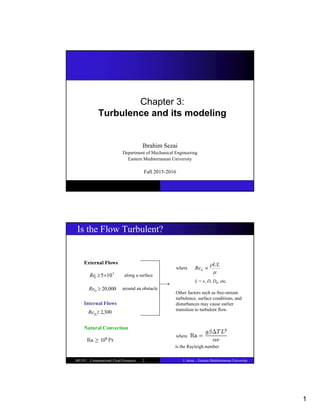
  • 1. 1 Chapter 3: Turbulence and its modeling Ibrahim Sezai Department of Mechanical Engineering Eastern Mediterranean University Fall 2015-2016 I. Sezai – Eastern Mediterranean University ME555 : Computational Fluid Dynamics 2 Is the Flow Turbulent? External Flows Internal Flows Natural Convection 5 10 5  x Re along a surface around an obstacle where  UL ReL  where Other factors such as free-stream turbulence, surface conditions, and disturbances may cause earlier transition to turbulent flow. L = x, D, Dh, etc. ,300 2  h D Re 20,000  D Re is the Rayleigh number
  • 2. 2 I. Sezai – Eastern Mediterranean University ME555 : Computational Fluid Dynamics 3 Introduction For Re > Recritical => Flow becomes Turbulent. Chaotic and random state of motion develops. Velocity and pressure change continuously with time The velocity fluctuations give rise to additional stresses on the fluid => these are called Reynolds stresses We will try to model these extra stress terms I. Sezai – Eastern Mediterranean University ME555 : Computational Fluid Dynamics 4 3.1 What is turbulence? ( ) ( ) u t U u t   
  • 3. 3 I. Sezai – Eastern Mediterranean University ME555 : Computational Fluid Dynamics 5 Two Examples of Turbulent Flow Larger Structures Smaller Structures In turbulent flows there are rotational flow structures called turbulent eddies, which have a wide range of length scales. I. Sezai – Eastern Mediterranean University ME555 : Computational Fluid Dynamics 6 In turbulent flow: A streak of dye which is introduced at a point will rapidly break up and dispersed  effective mixing Give rise to high values of diffusion coefficient for; - Mass - Momentum - and heat All fluctuating components contain energy across a wide range of frequencies or wave numbers 2 f wavenumber f frequency U   
  • 4. 4 I. Sezai – Eastern Mediterranean University ME555 : Computational Fluid Dynamics 7 Fig.3.3 Energy Spectrum of turbulence behind a grid I. Sezai – Eastern Mediterranean University ME555 : Computational Fluid Dynamics 8 Scales of turbulence 8  Largest eddies break up due to inertial forces  Smallest eddies dissipate due to viscous forces  Richardson Energy Cascade (1922)
  • 5. 5 I. Sezai – Eastern Mediterranean University ME555 : Computational Fluid Dynamics 9 Large Eddies: - have large eddy Reynolds number, - are dominated by inertia effects - viscous effects are negligible - are effectively inviscid Small Eddies: - motion is dictated by viscosity - Re ≈ 1 - length scales : 0.1 – 0.01 mm - frequencies : ≈ 10 kHz Energy associated with eddy motions is dissipated and converted into thermal internal energy  increases energy losses. - Largest eddies  anisotropic - Smallest eddies  isotropic vl  I. Sezai – Eastern Mediterranean University ME555 : Computational Fluid Dynamics 10 3.2 Transition from laminar to turbulent flow Can be explained by considering the stability of laminar flows to small disturbances  Hydrodynamic instability Hydrodynamic stability of laminar flows; a) Inviscid instability: flows with velocity profile having a point of inflection. 1. jet flows 2. mixing layers and wakes 3. boundary layers with adverse pressure gradients b) Viscous instability: flows with laminar profile having no point of inflection - occurs near solid walls
  • 6. 6 I. Sezai – Eastern Mediterranean University ME555 : Computational Fluid Dynamics 11 Fig. 3.4 Velocity profiles susceptible to a) Inviscid instability and b) Viscous instability I. Sezai – Eastern Mediterranean University ME555 : Computational Fluid Dynamics 12 Transition to Turbulence Jet flow: (example of a flow with point of inflection in velocity profile) Fig. 3.5. transition in a jet flow
  • 7. 7 I. Sezai – Eastern Mediterranean University ME555 : Computational Fluid Dynamics 13 Boundary layers on a flat plate (Example with no inflection point in the velocity profile) The unstable two-dimensional disturbances are called Tolmien- Schlichting (T-S) waves Fig. 3.6 plan view sketch of transition processes in boundary layer flow over a flat plate I. Sezai – Eastern Mediterranean University ME555 : Computational Fluid Dynamics 14 Fig. 3.7 merging of turbulent spots and transition to turbulence in a natural flat plate boundary layer
  • 8. 8 I. Sezai – Eastern Mediterranean University ME555 : Computational Fluid Dynamics 15 Common features in the transition process: (i) The amplification of initially small disturbances (ii) The development of areas with concentrated rotational structures (iii) The formation of intense small scale motions (iv) The growth and merging of these areas of small scale motions into fully turbulent flows Transition to turbulence is strongly affected by: - Pressure gradient - Disturbance levels - Wall roughness - Heat transfer The transition region often comprises only a very small fraction of the flow domain  Commercial CFD packages often ignore transition entirely (classify the flow as only laminar or turbulent) I. Sezai – Eastern Mediterranean University ME555 : Computational Fluid Dynamics 16 3.3Effect of turbulence on time-averaged Navier-Stokes eqns In turbulent flow there are eddying motions of a wide range of length scales A domain of 0.1×0.1m contains smallest eddies of 10-100 μm size We need mesh points The frequency of fastest events ≈ 10 kHz Δt ≈ 100μs needed DNS of turbulent pipe flow of Re = 105 requires a computer which is 10 million times faster than CRAY supercomputer Engineers need only time-averaged properties of the flow Let’s see how turbulent fluctuations effect the mean flow properties 9 12 10 10 
  • 9. 9 I. Sezai – Eastern Mediterranean University ME555 : Computational Fluid Dynamics 17 Descriptors of Turbulent Flow Time average or mean First we define the mean Φ of a flow property φ as follows: The property φ can be thought of as the sum of a steady mean component Φ and fluctuation component φ' The time average of the fluctuations φ' is , by definition, zero: 0 1 ( ) t t dt t       (3.2) ( ) ( ) t t      0 1 ( ) 0 t t dt t          (3.3) I. Sezai – Eastern Mediterranean University ME555 : Computational Fluid Dynamics 18 Variance, r.m.s. and turbulence kinetic energy The spread of the fluctuations φ' about the mean Φ are measured by     1/2 2 2 0 1 t rms dt t                 The rms values of velocity components can be measured (e.g. by hot- wire anemometer) The kinetic energy k (per unit mass) associated with the turbulence is defined as 2 2 2 1 ( ) 2 k u v w       The turbulence intensity Ti is linked to the kinetic energy and a reference mean flow velocity Uref as follows: 1/ 2 (2/3 ) i ref k T U  (3.4a) (3.5) (3.6)     2 2 0 1 t dt t         variance and root mean square (r.m.s.) (3.4b)
  • 10. 10 I. Sezai – Eastern Mediterranean University ME555 : Computational Fluid Dynamics 19 Moments of different fluctuating variables The variance is also called the second moment of the fluctuations. If and with 0                   Their second moment is defined as 0 1 t dt t             If velocity fluctuations in different directions were independent random fluctuations, then would be equal to zero. However, although are chaotic, they are not independent. As a result the second moments are non-zero. , and u v u w v w       , and u v w    , and u v u w v w       (3.7) I. Sezai – Eastern Mediterranean University ME555 : Computational Fluid Dynamics 20 Higher order moments Third moment is related to skewness (asymmetry) of the distribution of the fluctuations: Third moment: 3 3 0 1 ( ) ( ) t dt t         Fourth moment: 4 4 0 1 ( ) ( ) t dt t         Fourth moment is related to kurtosis (peakedness) of the distribution of the fluctuations: (3.8) (3.9)
  • 11. 11 I. Sezai – Eastern Mediterranean University ME555 : Computational Fluid Dynamics 21 Correlation functions – time and space The autocorrelation function based on two measurements shifted by time τ is defined as ( ) R    ξ 0 1 ( ) ( ) ( ) ( ) ( ) t R t t t t dt t                       Similarly, the autocorrelation function based on two measurements shifted by a certain distance in function space is defined as 1 ( ) ( , ) ( , ) ( , ) ( , ) t t t R t t t t dt t                        x x ξ x x ξ ( ) R     (3.10) (3.11) I. Sezai – Eastern Mediterranean University ME555 : Computational Fluid Dynamics 22 When τ = 0, or ξ = 0 and it is maximum because the two correlations are perfectly correlated. Since φ' is chaotic we expect that the fluctuations become increasingly decorrelated as τ or ξ → ∞ so, Rφ'φ'(∞) → 0. The eddies at the root of turbulence cause a certain degree of local structure in the flow, so there will be a correlation between the values of φ' at time t and a short time later or at a given location x and a small distance away. The decorrelation process will take place gradually over the lifetime (or size scale) of a typical eddy. The integral time and length scale represent concrete measures of the average period or size of a turbulent eddy. They can be computed from integrals of the autocorrelation functions Rφ'φ'(τ) or Rφ'φ'(ξ). By analogy it is also possible to define cross-correlation functions Rφ'ψ'(τ) or Rφ'ψ'(ξ) between pairs of different fluctuations. 2 (0) R      
  • 12. 12 I. Sezai – Eastern Mediterranean University ME555 : Computational Fluid Dynamics 23 Probability density function Probability density function P(φ*) is related to the fraction of time that a fluctuating signal spends between φ* and φ*+d φ*: * * * * * ( ) Prob( ) P d d           The average, variance and higher moments of the variables and its fluctuations are related to the probability density functions as follows: ( ) P d         ( ) ( ) ( ) n n P d             If n = 2  we get variance, if n = 3, 4,… we get higher order moments. (3.12) (3.13a) (3.13b) I. Sezai – Eastern Mediterranean University ME555 : Computational Fluid Dynamics 24 3.4. Characteristics of simple turbulent flows In turbulent thin shear layers, The following 2D incompressible turbulent flows with constant P will be considered: Free turbulent flows - Mixing layers - Jet - Wake Boundary layer near solid walls - Flat plate boundary layer - Pipe flow Data for U, will be reviewed. These can be measured by 1) Hot wire anemometry 2) Laser doppler anemometers This image cannot currently be displayed. 1 x y L        2 2 2 , , u v w and u v             
  • 13. 13 I. Sezai – Eastern Mediterranean University ME555 : Computational Fluid Dynamics 25 3.4.1 Free turbulent flows b= cross sectional layer width, y=distance in cross-stream direction x=distance downstream the source max min max max min max min for jets for mixinglayers for wakes U U U U U y y y g f h U b U U b U U b                          I. Sezai – Eastern Mediterranean University ME555 : Computational Fluid Dynamics 26 Eddies of a wide range of length scales are visible Fluid from surroundings is entrained into the jet.
  • 14. 14 I. Sezai – Eastern Mediterranean University ME555 : Computational Fluid Dynamics 27 If x is large enough  functions f, g and h are independent of x.  such flows are called self – preserving. The turbulence structure also reaches a self-preserving state albeit after a greater distance from the flow source than the mean velocity. Then Uref= Umax – Umin for a mixing layer and wakes Uref= Umax for jets Form of functions f, g, h and fi varies from flow to flow See Fig.3.10 2 2 2 1 2 3 4 2 2 2 2 ref ref ref ref u y v y w y uv y f f f f U b U b U b U b                                  I. Sezai – Eastern Mediterranean University ME555 : Computational Fluid Dynamics 28 Fig. 3.10 mean velocity distributions and turbulence properties for (a) two- dimensional mixing layer, (b) planar turbulent jet and (c) wake behind a solid strip
  • 15. 15 I. Sezai – Eastern Mediterranean University ME555 : Computational Fluid Dynamics 29 In Fig.3.10: are maximum when is maximum u' gives the largest of the normal stresses (v´and w´) .  Fluctuating velocities are not equal anisotropic structure of turbulence As mean velocity gradients tend to zero turbulence quantities tend to zero turbulence can’t be sustained in absence of shear The mean velocity gradient is also zero at the centerline of jets and wakes.No turbulence there. The value of is zero at the centerline of a jet and wake since shear stress must change sign here. u y   2 2 2 , u v and w and u v       2 max 0.15 0.40 u u    u v    I. Sezai – Eastern Mediterranean University ME555 : Computational Fluid Dynamics 30 3.4.2 Flat plate boundary and pipe flow y: distance away from the wall Near the wall (y small) is small viscous forces dominate Away from the wall (y large) is large inertia forces dominate. Near the wall U only depends on y, ρ, μ and τ (wall shear stress), so Dimensional analysis shows that Formula (3.18) is called the law of the wall Re inertia forces viscous forces  Re Uy v  Rey Rey ( , , , ) w U f y     ( ) u y U u f f y u                (3.16)   1/2 1/2 ( / 2) friction velocity w f u V C      
  • 16. 16 I. Sezai – Eastern Mediterranean University ME555 : Computational Fluid Dynamics 31 Far away from the wall: Dimensional analysis yields The most useful form emerges if we view the wall shear stress as the cause of a velocity deficit Umax – U which decreases the closer we get to the edge of the boundary layer or the pipe centerline. Thus This formula is called the velocity – defect law. ( , , , ) w U g y independent of      U y u g u           max U U y g u          (3.17) I. Sezai – Eastern Mediterranean University ME555 : Computational Fluid Dynamics 32 Linear sub layer – the fluid layer in contact with smooth wall Very near the wall there is no turbulent (Reynolds) shear stresses  flow is dominated by viscous shear For shear stress is approximately constant, Integrating and using U = 0 at y = 0, After some simple algebra and making use of the definitions of u+ and y+ this leads to Because of the linear relationship between velocity and distance from the wall the fluid layer adjacent to the wall is often known as the linear sub-layer ( 5) y  ( ) w U y y        w y U    u y    (3.18)
  • 17. 17 I. Sezai – Eastern Mediterranean University ME555 : Computational Fluid Dynamics 33 Log-law layer – the turbulent region close to smooth wall Outside the viscous sublayer (30 < y+ < 500) a region exists where viscous and turbulent effects are both important. The shear stress τ varies slowly with distance; it is assumed to be constant and equal to τw Assuming a length scale of turbulence lm = κy where lm is mixing length, the following relationship can be derived: κ = 0.4, B=5.5, E=9.8; (for smooth walls) B decreases with roughness κ and B are universal constants valid for all turbulent flows past smooth walls at high Reynolds numbers. (30 < y+ < 500)  log – law layer 1 1 ln ln( ) u y B Ey         (3.19) I. Sezai – Eastern Mediterranean University ME555 : Computational Fluid Dynamics 34 Outer layer – the inertia dominated region far from the wall Experimental measurements show that the log-law is valid in the region 0.02 < y ⁄ δ < 0.2. For larger values of y the velocity-defect law (3.19) provides the correct form. In the overlap region the log-law and velocity-defect law have to become equal. Tennekes and Lumley (1972) show that a matched overlap is obtained by assuming the following logarithmic form: where A is constant See Fig.3.11 max 1 ln U U y A Law of the Wake u            (3.20)
  • 18. 18 I. Sezai – Eastern Mediterranean University ME555 : Computational Fluid Dynamics 35 - The inner region: 10 to 20% of the total thickness of the wall layer; the shear stress is (almost) constant and equal to the wall shear stress τw. Within this region there are three zones - the linear sub-layer: viscous stresses dominate the flow adjacent to the surface - the buffer layer: viscous and turbulent stresses are of similar magnitude - the log-law layer: turbulent (Reynolds) stresses dominate. - The outer region or law-of-the-wake layer: inertia dominated core flow far from wall; free from direct viscous effects. Fig.3.11 I. Sezai – Eastern Mediterranean University ME555 : Computational Fluid Dynamics 36 For y ⁄ δ > 0.8 fluctuating velocities become almost equal isotropic turbulence structure here. (far away the wall) For y ⁄ δ < 0.2 large mean velocity gradients high values of .(high turbulence production) . Turbulence is anisotropic near the wall. 2 2 2 , u v and w and u v      
  • 19. 19 I. Sezai – Eastern Mediterranean University ME555 : Computational Fluid Dynamics 37 Rules which govern the time averages of fluctuation properties and : . 0; ; ; ; ; ; 0 ds ds s s                                                       Control volume in a 2D turbulent shear flow Fluid entering from top into the CV will bring in higher momentum fluid and will accelerate the slower moving layer. As a result, the fluid layer will experience additional turbulent shear stresses which are known as the Reynolds stresses. I. Sezai – Eastern Mediterranean University ME555 : Computational Fluid Dynamics 38 Since div and grad are both differentiations the above rules can be extended to a fluctuating vector quantity a = A + a' and its combinations with a fluctuating scalar : To illustrate the influence of turbulent fluctuations on mean flow we consider Substitute         ; ; div div div div div div div grad div grad              a A a a a (3.22)       0 1 1 1 div u p div u v div grad u t x v p div v vdiv grad v t y w p div w vdiv grad w t z                             u u u u (3.24a) (3.23) (3.24b) (3.24c ) ; ; ; ; u U u v V v w W w p P p                u U u     
  • 20. 20 I. Sezai – Eastern Mediterranean University ME555 : Computational Fluid Dynamics 39 Consider continuity equation: note that this yields the continuity equation A similar process is now carried out on the x-momentum equation (3.9a). The time averages of the individual terms in this equation can be written as follows: Substitution of these results gives the time-average x-momentum equation     ; ( ) 1 1 ; u U div u div U div u t t p P vdiv grad u vdiv gradU x x                    u U u 0 div  U (3.25) div div  u U 1 ( ) ( ) ( ) ( ) ( ) ( ) ( ) U P div U div u vdiv gradU t x I II III IV V             U u (3.26a) I. Sezai – Eastern Mediterranean University ME555 : Computational Fluid Dynamics 40 Repetition of this process on equations (3.9b) and (3.9c) yields the time-average y-momentum and z-momentum equations The process of time averaging has introduced new terms (III). Their role is additional turbulent stresses on the mean velocity components U, V and W. 1 ( ) ( ) (I) (II) (III) (IV) (V) 1 ( ) ( ) (I) (II) (III) (IV) (V) V P div V div v vdiv gradV t y W P div W div w vdiv gradW t z                         U u U u (3.26b) (3.26c)
  • 21. 21 I. Sezai – Eastern Mediterranean University ME555 : Computational Fluid Dynamics 41 Placing these terms on the rhs: 2 1 ( ) U P u u v u w div U v div gradU t x x y z                                 U (3.27a) 2 1 ( ) V P u v v v w div V v div gradV t y x y z                                 U (3.27b) 2 1 ( ) W P u w v w w div W v div gradW t z x y z                                 U (3.27c) Reynolds equations I. Sezai – Eastern Mediterranean University ME555 : Computational Fluid Dynamics 42 The extra stress terms result from six additional stresses, three normal stresses and three shear stresses: -These extra turbulent stresses are termed the Reynolds stresses. -The normal stresses are always non-zero -The shear stresses are also non-zero If, for example, u' and v' were statistically independent fluctuations, the time average of their product would be zero Similar extra turbulent transport terms arise when we derive a transport equation for an arbitrary scalar quantity. The time average transport equation for scalar φ is 2 2 2 xx yy zz xy yx xz zx yz zy u v w u v u w v w                                        (3.28a) * ( ) ( ) u v w div div grad S t x y z                                    U (3.29) 2 2 2 , and u v w          , and u v u w v w             u v   (3.28b)
  • 22. 22 I. Sezai – Eastern Mediterranean University ME555 : Computational Fluid Dynamics 43 In compressible flow density fluctuations are usually negligible The density-weighted averaged (or Favre-averaged) form of the compressible turbulent flow are: I. Sezai – Eastern Mediterranean University ME555 : Computational Fluid Dynamics 44 Closure problem – the need for turbulence modeling In the continuity and Navier – Stokes equations (3.8) and (3.9 a-c) there are 6 additional unknowns  the Reynolds stresses Similarly in scalar transport eqn (3.14) there are 3 extra unknowns: Main task of turbulence modeling: is to develop computational procedures to predict the 9 extra terms. (Reynolds stresses and scalar transport terms). , u v and w         
  • 23. 23 I. Sezai – Eastern Mediterranean University ME555 : Computational Fluid Dynamics 45 3.5 Turbulence models We need expressions for : - Reynolds stresses: - Scalar transport terms : 2 2 2 ' , , , , , u u v u w v v w w         , u v and w          I. Sezai – Eastern Mediterranean University ME555 : Computational Fluid Dynamics 46 Classical models: use the Reynolds eqn’s.(all commercial CFD codes) Large eddy simulation: the flow eqn’s are solved for the - mean flow and largest eddies - but the effect of the smaller eddies are modeled - are at the research state - calculations are too costly for engineering use.
  • 24. 24 I. Sezai – Eastern Mediterranean University ME555 : Computational Fluid Dynamics 47 energy cascade (Richardson, 1922) Turbulence Scales and Prediction Methods I. Sezai – Eastern Mediterranean University ME555 : Computational Fluid Dynamics 48 The mixing length and k-ε models are the most widely used and validated. They are based on the presumption that “there exists an analogy between the action of viscous stresses and Reynolds stresses on the mean flow” Viscous stresses are proportional to the rate of deformation. For incompressible flow: Notation: i = 1 or j = 1  x-direction i = 2 or j = 2  y-direction i = 3 or j = 3  z-direction 2 j i ij ij j i u u s x x                   (2.31)
  • 25. 25 I. Sezai – Eastern Mediterranean University ME555 : Computational Fluid Dynamics 49 For example Turbulent stresses are found to increase as the mean rate of deformation increases. It was proposed by Boussinesq in 1877 that Reynolds stress could be linked to mean rate of deformation where This is similar to viscous stress equation except that μ is replaced by μt, where μt = turbulent (eddy) viscosity 1 2 12 2 1 xy u u u v x x y x                              2 3 j i ij i j t ij j i U U u u k x x                         (3.33) 2 j i ij ij j i U U s x x                   2 2 2 0.5( ) k u v w       I. Sezai – Eastern Mediterranean University ME555 : Computational Fluid Dynamics 50 Similarly; kinematic turbulent or eddy viscosity. Turbulent momentum transport is assumed to be proportional to mean gradients of velocity By analogy turbulent transport of a scalar is taken to be proportional to the gradient of the mean value of the transported quantity. In suffix notation we get where Γt is the turbulent diffusivity. We introduce a turbulence Prandtl / Schmidt number as / t t v    i t i u x          (3.34) t t t     (3.35)
  • 26. 26 I. Sezai – Eastern Mediterranean University ME555 : Computational Fluid Dynamics 51 Experiments in many flows have shown that Most CFD procedures use Mixing length models: Attempts to describe the turbulent stresses by means of simple algebraic formulae for μt as a function of position The k-ε models: Two transport eqn’s (PDE’s) are solved: 1. For the turbulent kinetic energy, k 2. For the rate of dissipation of turbulent kinetic energy, ε. Both models assume that μt is isotropic (same for u, v, and w equations) (i.e. the ratio between Reynolds stresses and mean rate of deformation is the same in all directions) 1 t   1 t   2 / ( constant) t C C k C           I. Sezai – Eastern Mediterranean University ME555 : Computational Fluid Dynamics 52 This assumption fails in many categories of flow. It is necessary to derive and solve transport eqn’s for the 6 Reynolds stresses themselves. ( ). These eqn’s contain: 1. Diffusion 2. Pressure strain 3. Dissipation terms whose individual effects are unknown and cannot be measured Reynolds stress equation models: Solves the 6 transport equations (PDE’s) for the Reynolds stress terms together with k and ε eqn’s., by making assumptions about - diffusion - pressure strain - and dissipation terms. 2 2 2 ' , , , , , u u v u w v v w w        
  • 27. 27 I. Sezai – Eastern Mediterranean University ME555 : Computational Fluid Dynamics 53 Algebraic stress models: Approximate the Reynolds stresses in terms of algebraic equations instead of PDE type transport equations. Is an economical form of Reynolds stress model. Is able to introduce anisotropic turbulence effects into CFD simulations I. Sezai – Eastern Mediterranean University ME555 : Computational Fluid Dynamics 54 3.5.1 Mixing length model where C is a dimensionless constant of proportionality. Turbulent viscosity is given by This works well in simple 2-D turbulent flows where the only significant Reynolds stress is and only significant velocity gradient is For such flows where c is dimensionless constant xy yx u v         t v C   (3.36) t C     U y   U c y      (3.37) 2 : turbulent velocity scale : length scale of largest eddies t m m m s s        
  • 28. 28 I. Sezai – Eastern Mediterranean University ME555 : Computational Fluid Dynamics 55 Combining (3.26) and (3.27) and absorbing C and c into a new length scale This is Prandtl’s mixing length model. The Reynolds stress is (3.38) 2 t m U v y     m  2 xy yx m U U u v y y                (3.39) I. Sezai – Eastern Mediterranean University ME555 : Computational Fluid Dynamics 56 The transport of scalar quantity φ is modeled as where Γt = μt ⁄ σt and vt is found from (3.28). σt = 0.9 for near wall flows σt = 0.5 for jets and mixing layers Rodi(1980) σt = 0.7 in axisymmetric jets In Table 3.3: y : distance from the wall κ = 0.41 von Karman’s constant (3.40) t v y         
  • 29. 29 I. Sezai – Eastern Mediterranean University ME555 : Computational Fluid Dynamics 57 I. Sezai – Eastern Mediterranean University ME555 : Computational Fluid Dynamics 58
  • 30. 30 I. Sezai – Eastern Mediterranean University ME555 : Computational Fluid Dynamics 59 3.5.2. The k – ε model If convection and diffusion of turbulence properties are not negligible (as in the case of recirculating flows), then the mixing length model is not applicable. The k-ε model focuses on the mechanisms that affect the turbulent kinetic energy. Some preliminary definitions:     2 2 2 2 2 2 1 mean kinetic energy 2 1 turbulent kineticenergy 2 ( ) instantaneous kinetic energy K U V W k u v w k t K k            I. Sezai – Eastern Mediterranean University ME555 : Computational Fluid Dynamics 60 To facilitate the subsequent calculations it is common to write the components of the rate of deformation sij and the stresses τij in tensor (matrix) form: - Using gives and xx xy xz xx xy xz ij yx yy yz ij yx yy yz zx zy zz zx zy zz s s s s s s s s s s                                 ( ) ij ij ij s t S s   ( ) ; ( ) ; ( ) ; 1 1 ( ) ( ) 2 2 1 ( ) ( ) 2 xx xx xx yy yy yy zz zz zz xy xy xy yx yx yx xz xz xz zx zx zx U u V v s t S s s t S s x x y y W w s t S s z z U V u v s t S s s t S s y x y x U W s t S s s t S s z x                                                                                    1 2 1 1 ( ) ( ) 2 2 yz yz yz zy zy zy u w z x V W v w s t S s s t S s z y z y                                              
  • 31. 31 I. Sezai – Eastern Mediterranean University ME555 : Computational Fluid Dynamics 61 The product of a vector a and a tensor bij is a vector c The scalar product of two tensors aij and bij is evaluated as follows Suffix notation: 1 x – direction 2 y – direction 3 z – direction   11 12 13 1 2 3 21 22 23 31 32 33 1 11 2 21 3 31 1 1 12 2 22 3 32 2 1 13 2 23 3 33 3 ij i ij T T j b b b b a b a a a b b b b b b a b a b a b c a b a b a b c c a b a b a b c                                           a c 11 11 12 12 13 13 21 21 22 22 23 23 31 31 32 32 33 33 ij ij a b a b a b a b a b a b a b a b a b a b           I. Sezai – Eastern Mediterranean University ME555 : Computational Fluid Dynamics 62 Governing equation for mean flow kinetic energy K Reynolds equations: (3.27a), (3.27b), (3.27c) Multiply x – component Reynolds eqn. (3.27a) by U Multiply y – component Reynolds eqn. (3.27b) by V Multiply z – component Reynolds eqn. (3.27c) by W Then add the result together. After some algebra the time-average eqn. for mean kinetic energy of the flow is
  • 32. 32 I. Sezai – Eastern Mediterranean University ME555 : Computational Fluid Dynamics 63 Or in words, for the mean kinetic energy K, we have   ( ) ( ) 2 2 ( ) ( ) ( ) ( ) ( ) ( ) ( ) ij i j ij ij i j ij K div K div P S u u S S u u S t I II III IV V VI VII                      U U U U (3.41) I. Sezai – Eastern Mediterranean University ME555 : Computational Fluid Dynamics 64 Governing equation for turbulent kinetic energy k 1- Multiply x, y and z momentum eqns (3.24a-c) by u´, v´ and w´,respectively 2- Multiply x, y and z Reynolds eqns (3.27a-c) by u´, v´ and w´, respectively 3- subtract the two of the resulting equations Rearrange:  yields the equation for turbulent kinetic energy k: ( ) 1 ( ) 2 2 2 ( ) ( ) ( ) ( ) ( ) ( ) ( ) ij i i j ij i j ij ij k div k div p s u u u s s u u S t I II III IV V VI VII                                    U u u (3.42)
  • 33. 33 I. Sezai – Eastern Mediterranean University ME555 : Computational Fluid Dynamics 65 The viscous term (VI) Gives a negative contribution to (3.32) due to the appearance of the sum of squared fluctuating deformation rate s'ij The dissipation of turbulent kinetic energy is caused by work done by the smallest eddies against viscous stresses. The rate of dissipation per unit mass (m2/s3) is denoted by The k – ε model equations: It is possible to develop similar transport eqns. for all other turbulence quantities The exact ε – equation, however, contains many unknown and unmeasurable terms The standard k – ε model(Launder and Spalding,1974) has two model eqns (a) one for k and (b) one for ε   2 2 2 2 2 2 11 22 33 12 13 23 2 2 2 2 2 ij ij s s s s s s s s                    2 ij ij vs s      (3.43) I. Sezai – Eastern Mediterranean University ME555 : Computational Fluid Dynamics 66 We use k and ε to define velocity scale and length scale representative of the large scale turbulence as follows: Applying the same approach as in the mixing length model we specify the eddy viscosity as follows where Cμ is a dimensionless constant  3/ 2 1/ 2 k k       2 t k C C        (3.44)
  • 34. 34 I. Sezai – Eastern Mediterranean University ME555 : Computational Fluid Dynamics 67 The standard model uses the following transport equations used for k and ε In words the equations are The equations contain five adjustable constants . The standard k – ε model employs values for the constants that are arrived at by comprehensive data fitting for a wide range of turbulent flows: ( ) ( ) 2 k t t ij ij k P k div k div grad k S S t                    U     (3.45) 2 1 2 ( ) ( ) 2 t t ij ij div div grad C S S C t k k                          U (3.46) 1 2 0.09; 1.00; 1.30; 1.44; 1.92 k C C C            (3.47) 1 2 , , , and k C C C       I. Sezai – Eastern Mediterranean University ME555 : Computational Fluid Dynamics 68 To compute the Reynolds stresses with the k – ε model (3.44-3.46), Boussinesq relationship is used: δij = 1 if i = j, δij = 0 if i ≠ j Contraction gives Using Then which is the definition of k. So an equal 1/3 is allocated to each normal stress component in eqn (3.48) to have –2ρk when summed. This implies an isotropic assumption for the normal Reynolds stresses. 2 2 2 3 3 j i i j t ij t ij ij j i U U u u k S k x x                            (3.48) 2 2 2 2 3 3 i i i i t ii t i i U U u u k k x x                  3 1 2 1 2 3 0 due to continuity i i U U U U x x x x             3 1 2 i i i u u k        1 1 2 2 3 3 1 where 2 i i i i k u u u u u u u u u u                    
  • 35. 35 I. Sezai – Eastern Mediterranean University ME555 : Computational Fluid Dynamics 69 B.C.’s for high Re model k and ε-equations The following boundary conditions are needed For inlet, if no k and ε is available crude approximations can be obtained from the - Turbulence intensity, Ti - Characteristic length, L (equivalent pipe diameter) : The formulae are closely related to the mixing length formulae in section 3.5.1 and the universal distributions near a solid wall given below.   3/ 2 2 3/4 2 ; ; 0.07 3 ref i k k U T C L        I. Sezai – Eastern Mediterranean University ME555 : Computational Fluid Dynamics 70 Wall boundary conditions for high Re models Near the wall, at high Reynolds numbers, equations (3.44-3.46) of the standard k – ε model are not integrated right to the wall. Instead, universal behaviour of near wall flows is used. In this region measurements of the budgets indicates that: the rate of turbulence production = rate of dissipation Using this assumption and , the following wall functions can be derived for a grid point P, which is nearest to the wall, in the region 30 < y+ < 500: where κ = 0.41 (Von Karman’s constant) E = 9.8 (wall roughness parameter) for smooth walls 1 ln for 30 500 u Ey y        (3.19)   2 3 1 ln ; ; for 30 500 P P P u u U u Ey k y u y C                 (3.49) 2 / t C k        1/2 friction velocity, w u y u y         
  • 36. 36 I. Sezai – Eastern Mediterranean University ME555 : Computational Fluid Dynamics 71 Wall b.c.’s for high Re models: Momentum Eqns Using k from Eqn. (3.49), 2 1/2 1/4 P P u k u k C C        1/2 1/4 P P P P k C y u y y          In the viscous sublayer, near the wall (y+ < 5) the flow is laminar and the velocity is given by u y    The position of the interface between the laminar sublayer and the log law layer can be found by equating Eqns. (3.18) and (3.19): (3.18) int int int 1 ln( ), 11.63 y Ey y        if 11.63 1 ln( ) if 11.63 P P P P P y y u Ey y               Then, the velocity at a point P near the wall is found from I. Sezai – Eastern Mediterranean University ME555 : Computational Fluid Dynamics 72 Wall b.c.’s for high Re models: k and ε-Eqns k-equation, Eqn. (3.45), is integrated right to the wall. However, the source term of the k-equation given by 2 k t ij ij k s S S P         is calculated at a near wall point P by assuming local equilibrium. Under this assumption, the rate of turbulence production = rate of dissipation. Thus, the rate of turbulence production is calculated from 2 1/2 1/4 1/4 1/2 , where , w k w w w P P P U P u u k C y C k y                 and ε is calculated from 3/4 3/2 P P P C k y    
  • 37. 37 I. Sezai – Eastern Mediterranean University ME555 : Computational Fluid Dynamics 73 Wall b.c.’s for high Re models: k and ε-Eqns The boundary condition for k imposed at the wall is / 0 k n    where n is normal to the wall. The ε-equation is not solved at the wall-adjacent cells but is computed from 3/4 3/2 P P P C k y     I. Sezai – Eastern Mediterranean University ME555 : Computational Fluid Dynamics 74 Wall b.c.’s for high Re models: Energy equation The wall heat flux is given by where T+ is calculated from the universal near wall temperature distribution valid at high Reynolds numbers (Launder and Spalding, 1974): Finally P is the “pee-function”, a correction function dependent on the ratio of laminar to turbulent Prandtl numbers (Launder and Spalding, 1974)   , , , , , with temperature at near wall point turbulent Prandtl number wall temperature / Prandtl number wall heat flux thermal conducti T l w P T t w T t p P T t w T l P T w T T T C u T u P q T y T C q                                         vity fluid specific heat and constant pressure p C  (3.50) 1/4 1/2 ( ) / w P P P w q C C k T T T      
  • 38. 38 I. Sezai – Eastern Mediterranean University ME555 : Computational Fluid Dynamics 75 Low Reynolds number k-ε models At low Reynolds numbers (which is the case near the wall) the constants Cμ, C1ε and C2ε in Eqns. (3.51–3.53) are not valid so these equations cannot be integrated right to the wall. To integrate the governing equations right to the wall, modifications to the standard k-ε model is necessary. The equations of the low Reynolds number k – ε model, which replace (3.44-3.46), are given below: ( ) ( ) 2 t t ij ij k k div k div grad k S S t                              U 2 t k C f       2 1 1 2 2 ( ) ( ) 2 t t ij ij div div grad t C f S S C f k k                                    U (3.51) (3.53) (3.52) I. Sezai – Eastern Mediterranean University ME555 : Computational Fluid Dynamics 76 Modifications: A viscous contribution is included Cμ, C1ε and C2ε are multiplied by wall damping functions fμ, f1 , f2 which are functions of turbulence Reynolds number or similar functions As an example we quote the Lam and Bremhorst (1981) wall- damping functions which are particularly successful: In function the parameter is defined by . Lam and Bremhorst use as a boundary condition. 0 y     2 3 2 1 2 20.5 1 exp( 0.0165Re ) 1 ; Re 0.05 1 ; 1 exp( Re ) y t t f f f f                              (3.54) 1/2 / k y v f Rey
  • 39. 39 I. Sezai – Eastern Mediterranean University ME555 : Computational Fluid Dynamics 77 Assessment of performance Table 3.4 k-ε model assessment I. Sezai – Eastern Mediterranean University ME555 : Computational Fluid Dynamics 78 k-ε Model Implementation Details The flow equations (3.27) can be written in tensor notation as       j i i i j i j j j j i j i j i i j j j i i U U U P U U u u t x x x x x x U U P u u x x x x                                                                          Inserting the Boussinesq relation (3.38) 2 3 j i ij i j t ij j i U U u u k x x                             * ( ) j i i i j t j j j i i U U U P U U t x x x x x                                      where P* = P + (2/3)ρk (3.54a) (3.54b) Note that Eqn. (3.54b) is the same as that of Navier-Stokes Eqns. given by (2.32a,b,c) with μ replaced by (μ + μt) and p by P*.
  • 40. 40 I. Sezai – Eastern Mediterranean University ME555 : Computational Fluid Dynamics 79 Rearranging     * * ( ) ( ) ( ) ( j i i i j t j j j i i j i t t j j j i i t j U U U P U U t x x x x x U U P x x x x x x                                                                             * * source term ) ( ) ( ) ( ) ( ) j j i t j j i j i i j i t t j j j i i U U U P x x x x x x U U P x x x x x                                                                      Note that we have used:   ( ) 0 0 (due to continuity if = constant, and the fluid is incompressible) j j j j i j i i j i U U U x x x x x x x                                            (3.54c) The terms after the first parenthesis on the RHS of Eqn. (3.54c) are treated as a source . I. Sezai – Eastern Mediterranean University ME555 : Computational Fluid Dynamics 80 k-ε Model Equations in Generic Form * ( ) ( ) ( ) Equation Continuity 1 0 0 x-Momentum y-Momentum eff eff eff eff eff eff eff div div grad s t s U V W P U x x y x z x x U V V x y y                                                                        U * * 2 1 1 2 2 z-Momentum Energy 0 Turbulence ke Dissipation of ke eff eff eff eff eff t t t k k t k ij ij W P y z y y U V W P W x z y z z z z T k P C f P C f k k U S S x                                                                                          2 2 2 2 2 2 3 * 2 1 1 1 1 1 , 2 2 2 2 (2 / 3) , , / , 1 0.05 / , 2 j i ij j i eff t t k t U U V W U V W U V W S y z y x x z z y x x P P k C f k f f P                                                                                                 2 2 2 2 1/2 1 exp 0.0165Re 1 20.5 / Re , 1 exp( Re ), Re / , = minimum distance to the nearest wall Re / , 0.09, 1.00, 1.30, j i i ij ij t j i j y t t t y k t U U U S S x x x f f k y k y C                                             1 2 0.9, 1.44, 1.92, Pr C C       The low Reynolds number k-ε model equations can be written in generic form as
  • 41. 41 I. Sezai – Eastern Mediterranean University ME555 : Computational Fluid Dynamics 81 Source term linearization in k-ε models When the source term is linearized as C P P s s s    1) sP must be negative for a convergent iterative solution, which ensures diagonal dominance of the coefficient matrix. This is a requirement for the boundedness criteria discussed in chapter 5. 2) sC must be positive (and sP must be negative ) to obtain all positive  values. (Patankar, 1980) Both k and ε are strictly positive quantities. So, to obtain always positive results for k and ε, the source terms should be formulated such that sC is positive and sP is negative for k and ε equations. I. Sezai – Eastern Mediterranean University ME555 : Computational Fluid Dynamics 82 Source term linearization in k equation k-equation: Consider first term, ρPk. Inserting into Pk k k s P    2 / t C f k       2 2 3 2 2 k t ij ij ij ij k P S S C f S S C k         Linearization of ρPk in the form of sk = sPP + sC would give . However, since C3 > 0 and k > 0, then sP > 0, which violates the boundedness criteria. We can conclude that positive terms (e.g. Pk) cannot be linearized using such an implicit manner. As a result, Pk should be put into sC. Consider the second term, –ρε. From . Inserting Pk and ε into the source term , gives: 3 and 0 P C s C k s   2 / t C f k       2 / t C f k       k k s P   
  • 42. 42 I. Sezai – Eastern Mediterranean University ME555 : Computational Fluid Dynamics 83 Source term linearization in k-equation k-equation: 2 2 2 2 , , k k k k t t C f C f s P P k b ak b P a                  For the second term, ak2, the linearization proposed by Patankar (1980) can be used:       * * * * 2 * * * 2 * ( ) 2 ( ) 2 P P P P P P P P P ds s s k k b a k ak k k b a k ak k dk                     2 2 * 2 * 2 * * ( ) ( ) and 2 2 C P k P P P P t t C f C f s b a k P k s ak k                 Then, where the superscript * refers to the previous iteration values. However, this linearization does not yield a robust algorithm. A better approach is to put the coefficient of k to the sP term. Comparing sk relation with gives: C P P s s s     2 * * ( ) ( ) C k k P k t s b P C f s ak k           I. Sezai – Eastern Mediterranean University ME555 : Computational Fluid Dynamics 84 Positivity of sC term in k-equation For consistency, the turbulent viscosity, t, should be a positive quantity. However, t may become negative if ε becomes negative during iterations. t should be enforced to take positive values during iterations. The limiter used for enforcing positive values for t is given later in Eqn. (3.51b). 2 t C f k      
  • 43. 43 I. Sezai – Eastern Mediterranean University ME555 : Computational Fluid Dynamics 85 Source term linearization in ε-equation ε-equation: 2 2 1 1 2 2 1 1 2 2 where , / k k s C f P C f b a k k b C f P a C f k k                  Note that, since b > 0, it cannot be linearized impicitly as it gives a positive sP. The second term, aε2, can be linearized by transferring the coefficient of the variable ε to the sP term, in accordance with Then, for  =  we obtain: where the superscript * refers to the previous iteration values. C P P s s s     * 1 1 * * 2 2 * ( ) ( ) C k P s b C f P k s a C f k               I. Sezai – Eastern Mediterranean University ME555 : Computational Fluid Dynamics 86 Source term linearization in ε-equation The source terms sP and sC of the ε-equation can be written in terms of eddy viscosity μt using 2 t t C f k C f k k              which yields * 1 1 * 2 2 ( ) ( ) C k t P t C f k s b C f P C f k s a C f                    
  • 44. 44 I. Sezai – Eastern Mediterranean University ME555 : Computational Fluid Dynamics 87 Positivity of sC term in k- and ε-equations sC term should be positive to obtain positive values during the iteration of a general variable . Rewriting the sC term for the k- equation: We observe that, (sC)k is positive if μt is enforced to take positive values since Pk is always positive. Rewriting the sC term for the -equation: Again, we observe that, (sC) is positive if μt is enforced to take positive values. Then, enforcing μt to take positive values is necessary to obtain positive results during iterations of both k- and -equations. ( ) 2 C k k t ij ij s P S S    * 1 1 ( ) C k t C f k s C f P        I. Sezai – Eastern Mediterranean University ME555 : Computational Fluid Dynamics 88 Limiting of eddy viscosity μt Note that both k and ε are strictly positive quantities. However, during iterations, undershoots may develop which will result in negative values for either k or ε which will give negative μt values in accordance with Eqn. (3.51):. (3.51) Also if ε → 0, division by zero will occur in accordance with Eqn. (3.51). Also, sP and sC terms of both k and ε-equations contain 1/μt term so that if μt → 0, division by zero will occur. To overcome these difficulties μt is limited to a small fraction of laminar viscosity μl by using (3.51b) 2 / t C f k       2 4 max ,10 t l k C f              
  • 45. 45 I. Sezai – Eastern Mediterranean University ME555 : Computational Fluid Dynamics 89 3.5.3 Reynolds stress equation models The most complex classical turbulence model is Reynolds stress equation model (RSM), Also called : - second order - or second – moment closure model Drawbacks of k – ε model emerge when it is attempted to predict - flows with complex strain field - flows with significant body forces The exact Reynolds stress transport eqn can account for the directional effects of the Reynolds stress field. Let (Reynolds stress) ij ij i j R u u        I. Sezai – Eastern Mediterranean University ME555 : Computational Fluid Dynamics 90 The exact solution for the transport of takes the following form Equation (3.45) describes six partial differential equations: one for the transport of each of the six independent Reynolds stresses ( ) Two new terms appear compared with ke eqn (3.32) 1. . : pressure strain correction term 2. . : rotation term ij ij ij ij ij ij DR P D Dt         (3.55) 2 2 2 1 2 3 1 2 1 3 2 3 2 1 1 2 3 1 1 3 3 2 2 3 , , , , ,since , u u u u u u u and u u u u u u u u u u and u u u u                         ij  ij  ij R
  • 46. 46 I. Sezai – Eastern Mediterranean University ME555 : Computational Fluid Dynamics 91 The convective term is The production term is The rotation term is where ( ) ( ) k i j ij i j k U u u C div u u x           U (3.56) (3.57) (3.58) j i ij im jm m m U U P R R x x              2 ( ) ij k j m ikm i m jkm u u e u u e          rotation vector 1 if , and are different and in cyclic order 1 if , and are different and in anti-cyclic order 0 if any two indices are the same k ijk ijk ijk e i j k e i j k e        I. Sezai – Eastern Mediterranean University ME555 : Computational Fluid Dynamics 92 The diffusion term Dij can be modelled by the assumption that the rate of transport of Reynolds stresses by diffusion is proportional to gradient of Reynolds stress. The dissipations rate εij is modeled by assuming isotropy of the small dissipative eddies. It is set so that it effects the normal Reynolds stresses (i = j) only and in equal measure. This can be achieved by where ε is the dissipation rate of turbulent kinetic energy defined by (3.43). The Kronecker delta, δij is given by δij = 1 if i = j and δij = 0 if i ≠ j   2 with ; 0.09 1.0 ij t t ij ij m k m k t k R v v D div grad R x x k v C C and                            (3.59) 2 3 ij ij    (3.60)
  • 47. 47 I. Sezai – Eastern Mediterranean University ME555 : Computational Fluid Dynamics 93 For Πij term: The pressure – strain interactions are the most difficult to model Their effect on the Reynolds stresses is caused by two distinct physical processes: 1. Pressure fluctuations due to two eddies interacting with each other 2. Pressure fluctuations due to the interactions of an eddy with a region of flow of different mean velocity Its effect is to make Reynolds stresses more isotropic and to reduce the Reynolds shear stresses Measurements indicate that; The wall effect increases the isotropy of normal Reynolds stresses by damping out fluctuations in the directions normal to the wall and decreases the magnitude of the Reynolds shear stresses. I. Sezai – Eastern Mediterranean University ME555 : Computational Fluid Dynamics 94 A comprehensive model that accounts for all these effects is given in Launder et al (1975). They also give the following simpler form favoured by some commercial available CFD codes: Turbulent kinetic energy k is 1 2 1 2 2 2 3 3 with 1.8; 0.6 ij ij ij ij ij C R k C P P k C C                            2 2 2 11 22 33 1 2 3 1 1 2 2 k R R R u u u          (3.61)
  • 48. 48 I. Sezai – Eastern Mediterranean University ME555 : Computational Fluid Dynamics 95 The six equations for Reynolds stress transport are solved along with a model equation for the scalar dissipation rate ε. Again a more exact form is found in Launder et al (1975), but the equation from the standard k – ε model is used in commercial CFD for the sake of simplicity (3.62) 2 1 1 2 1 2 2 where 1.44 and 1.92 t t ij ij v D div grad C f v S S C Dt k k C C                       I. Sezai – Eastern Mediterranean University ME555 : Computational Fluid Dynamics 96 Boundary conditions for the RSM model The usual boundary conditions for elliptic flows are required for the solution of the Reynolds stress transport equations: inlet: specified distributions of Rij and ε outlet and symmetry: ∂Rij /∂n = 0 and ∂ ε/∂n = 0 free stream: Rij = 0 and ε = 0 are given or, ∂Rij /∂n = 0 and ∂ ε/∂n = 0 solid wall: use wall functions relating Rij to either k or (uτ)2 e.g. In the absence of any information, inlet distributions are calculated from where ℓ is the characteristic length of the equipment (e.g. pipe diameter) 2 2 2 1 2 3 1 2 1.1 , 0.25 , 0.66 , 0.26 u k u k u k u u k             3 / 2 2 3 / 4 2 2 2 1 2 3 2 ; ; 0.07 ; 3 1 ; ; 0 ( ) 2 ref i i j k k U T C L u k u u k u u i j                 
  • 49. 49 I. Sezai – Eastern Mediterranean University ME555 : Computational Fluid Dynamics 97 Boundary conditions for RSM model For computations at high Reynolds numbers wall-function-type boundary conditions can be used which are very similar to those of the k-ε model . Near wall Reynolds stress values are computed from formulae such as where cij are obtained from measurements. Low Reynolds number modifications to the model can be incorporated to add the effects of molecular viscosity to the diffusion terms and to account for anisotropy in the dissipation rate in the Rij-equations. Wall damping functions to adjust the constants of the ε-equation and a modified dissipation rate variable give more realistic modeling near solid walls. ij i j ij R u u c k     1/ 2 2 ( 2 ( / ) ) v k y        I. Sezai – Eastern Mediterranean University ME555 : Computational Fluid Dynamics 98 Similar models exist for the 3 scalar transport terms of eqn (3.32) in the form of PDE’s. In commercial CFD codes a turbulent diffusion coefficient is added to the laminar diffusion coefficient, where for all scalars. / t t      0.7    i u  
  • 50. 50 I. Sezai – Eastern Mediterranean University ME555 : Computational Fluid Dynamics 99 Assessment of RSM model Table 3.6 Reynolds stress equation model assessment. I. Sezai – Eastern Mediterranean University ME555 : Computational Fluid Dynamics 100 Asssesment of performance of RSM model Figure 3.16 Comparison of predictions of RSM and standard k-ε model with measurements on a high-lift Aerospatiale aerofoil: (a) pressure coefficient; (b) skin friction coefficient Source: Leschziner, in Peyret and Krause (2000)
  • 51. 51 I. Sezai – Eastern Mediterranean University ME555 : Computational Fluid Dynamics 101 Incorrect usage of the terms: High and low Reynolds number High or low Reynolds number turbulence models do not necessarily refer to models which are used to simulate flows having high or low speeds. In this usage of the term, the Reynolds number is based on the distance from the wall. In the near-wall region the flow velocity and distance to the wall is low so that the Reynolds number is low. Then, low Reynolds number models refer to turbulence models which can simulate the flow in near-wall region where the viscous effects dominate, by integrating the equations right to the wall, without resorting to wall functions. High Reynolds number models on the other hand refer to models which can simulate the flow in the fully turbulent region only, where the Reynolds number is high. In this region the turbulence effects dominate over the viscous effects. The model equations are not valid in the near wall region. As a result, high Reynolds number model equations are not integrated right to the wall. These models use wall functions to find the variables in the near wall region. I. Sezai – Eastern Mediterranean University ME555 : Computational Fluid Dynamics 102 Shortcomings of two-equation models such as k-ε model Low Reynolds number flows: Very rapid changes occur in the distribution of k and ε as we reach the buffer layer between the fully turbulent region and the viscous sublayer. To force the rapid changes to k and ε, the constants of the high Reynolds number model are multiplied by exponential damping functions which require large number of grid points to resolve the changes. As a result, the system of equations become stiff which makes the numerical solution difficult to converge. Rapidly changing flows: The Reynolds stress is proportional to Sij in two-equation models. This only holds in equilibrium flows where the rates of production and dissipation of k are roughly in balance. In rapidly changing flows this is not true. i j u u    
  • 52. 52 I. Sezai – Eastern Mediterranean University ME555 : Computational Fluid Dynamics 103 Shortcomings of two-equation models such as k-ε model Stress anisotropy: Two equation model predicts normal stresses which are all approximately equal to –⅔ρk if a thin shear layer is simulated. Experimental data presented in section 3.4 showed that this is not correct. In spite of this the k-e model performs well in such flows because the gradients of normal turbulent stresses are small compared with the gradient of the dominant turbulent shear stress . In more complex flows the gradients of normal turbulent stresses are not negligible and can drive significant flows. These effects can not be predicted by the two equation models. Strong adverse pressure gradients and recirculation regions: This problem is also attributable to the isotropy of the predicted normal stresses of the k-ε model. The k-ε model overpredicts the shear stress and suppresses separation in flows over curved walls. This is a significant problem in flows over airfoils, e.g. in aerospace applications. 2 i u    2 i u    u v     I. Sezai – Eastern Mediterranean University ME555 : Computational Fluid Dynamics 104 Shortcomings of two-equation models such as k-ε model Extra strains: Streamline curvature, rotation and extra body forces all give rise to additional interactions between the mean strain rate and the Reynolds stresses. These physical effects are not captured by standard two-equation models. RSM model addresses most of these problems adequately, but at the cost of additional storage and computer time. Below we consider some of the more recent advances in turbulence modeling that seek to address some or all of the above problems.
  • 53. 53 I. Sezai – Eastern Mediterranean University ME555 : Computational Fluid Dynamics 105 Advanced turbulence models Advanced treatment of the near-wall region: two-layer k-ε model The numerical instability problems associated with the wall damping functions used in low Reynolds number k-ε models are avoided by subdividing the boundary layer into two regions (Jongen,1997): 1) Fully turbulent region: In this region the standard k-ε model is used where the eddy viscosity is defined by Eqn. (3.44); 2) Viscous region, Red < Red *: Only the momentum equations and the k-equation is solved (Eqn.3.45). Turbulent viscosity in this viscous region is calculated from and ε is calculated from where * * Re / Re , Re 50 200 d d d y k      2 , / t t C k      3/2 / k     1/2 , t v C k      I. Sezai – Eastern Mediterranean University ME555 : Computational Fluid Dynamics 106 Two-layer k-ε model The length scales ℓμ and ℓε contain necessary damping effects in the near wall region and are taken from the one–equation model of Wolfshtein (1969): where y is the normal distance to the wall. In order to avoid instabilities associated with differences between μt,t and μt,v at the join between the fully turbulent and viscous regions, a blending formula is used to evaluate the eddy viscosity in   1 exp( Re / 1 exp( Re / l d l d C y A C y A                 3/4 1/2 , 2 , Re / l l d C C A C k d         2 2 / 3 ij i j t ij ij u u S k           
  • 54. 54 I. Sezai – Eastern Mediterranean University ME555 : Computational Fluid Dynamics 107 The turbulent viscosity is calculated from where The blending function λε is zero at the wall and tends to 1 in the fully turbulent region when Red >> Red *. The constant A can be adjusted in order to control the sharpness of the transition from one model to the other. For example A =1,…,10 leads to transitions occurring within a few cells, smaller values giving sharper transitions. , , (1 ) t t t t v           * Re Re 1 1 tanh 2 d d A                  I. Sezai – Eastern Mediterranean University ME555 : Computational Fluid Dynamics 108 Comparison of two-layer k-ε model with various turbulence models in predicting Cp = (P2–P1) / (ρU1 2) in a 2-D diffuser, (Jongen, 1997). Geometry of the diffuser. (Jongen, 1997) Profiles of ε at the exit section of the diffuser (θ = 10), for different values of the switching parameter Red * between the two layers, (Jongen, 1997).
  • 55. 55 I. Sezai – Eastern Mediterranean University ME555 : Computational Fluid Dynamics 109 Strain sensitivity: RNG k-ε model RNG k - ε model (Renormalization Group). The RNG procedure: systematically removes the small scales of motion from the governing equations by expressing their effects in terms of large scale motions and a modified viscosity. (Yakhot et al 1992): RNG k-ε model equations for high Reynolds number flows:   ( ) ( ) k eff ij ij k div k div grad k S t              U   2 * 1 1 2 2 2 1 ( ) ( ) with 2 2 / 3 and ; and 0.0845; 1.39; 1.42; eff ij ij ij i j t ij ij eff t t k div div grad C f S C f t k k u u S k k C C C                                                  U 2 1.68 C   (3.65) (3.67) (3.66)     1/2 0 * 1 1 0 3 1 / and ; 2 ; 4.377; 0.012 1 ij ij k C C S S                   I. Sezai – Eastern Mediterranean University ME555 : Computational Fluid Dynamics 110 Only the constant β is adjustable; the above value is calculated from near wall turbulent data. All other constants are explicitly computed as part of the RNG process. The ε-equation has long been suspected as one of the main sources of accuracy limitations for the standard version of the k-ε model and the RSM. It is, therefore, interesting to note that the model contains a strain-dependent correction term in the constant C1ε of the production term in the RNG model ε-equation. Its performance is better than the k-ε model for an expanding duct, but actually worse for a contraction with the same ratio.
  • 56. 56 I. Sezai – Eastern Mediterranean University ME555 : Computational Fluid Dynamics 111 Spalart-Allmaras model Has only one transport equation for kinematic eddy viscosity parameter . Turbulent eddy viscosity is computed from (3.68) where fv1 is the wall damping function given by which tends to unity for high Reynolds number flows ( ). and fv1 → 0 at the wall. The Reynolds stresses are computed from (3.69)  1 t v f     3 1 3 3 1 ; v v f c          t     1 2 j i ij i j t ij v j i U U u u S f x x                         I. Sezai – Eastern Mediterranean University ME555 : Computational Fluid Dynamics 112 The transport equation for is as follows:  2 2 1 1 ( ) ( ) ( ) ( ) (I) (II) (III) (IV) (V) (VI) b b w w k k div div grad C C C f t x x y                                      U          Transport Transport of Rate of Rate of Rate of change of by byturbulent production dissipation of convection diffusion of of               (3.70) 2 2 ( ) where 2 mean vorticity 1 mean vorticity tensor 2 v ij ij j i ij j i f y U U x x                              1/6 6 3 2 6 6 1 3 1 1 , wall damping functions 1 w v w v w c f f g f g c              
  • 57. 57 I. Sezai – Eastern Mediterranean University ME555 : Computational Fluid Dynamics 113 In the k-ε model the length scale is ℓ = k3/2/ε. In a one-equation model ℓ cannot be computed since there is no transport equation for k and ε. However, ℓ should be specified to determine the dissipation rate. Inspection of Eqn. (3.70) reveals that ℓ = κy has been used as a length scale. This is also the mixing length used in developing the log-law for wall boundary layers. The constants are: The model gives good performance for flows with adverse pressure gradients. In complex geometries it is difficult to determine the length scale, so the model is unsuitable for more general internal flows. 2 2 1 2 1 1 6 2 2 3 2 2 1 2 / 3, 0.4187, 0.1355, 0.622, ( ), min ,10 , 0.3, 2 b v b b w b v w w w C C C C C g r C r r r C C y                             I. Sezai – Eastern Mediterranean University ME555 : Computational Fluid Dynamics 114 Wilcox k-ω model In the k-ε model the kinematic eddy viscosity is expressed as However, ε is not the only possible length scale determining variable. In fact, k-ω model (Wilcox,1994) uses ω = ε / k as the second variable. Then, the length scale is ℓ = (k)1/2 / ε and (3.71) The Reynolds stresses are computed from Boussinesq expression: (3.72) The transport equation for k and ω for turbulent flow at high Reynolds is: 3/2 , velocity scale, / length scale t k k          / t k     2 2 2 3 3 j i ij i j t ij ij t ij j i U U u u S k k x x                              * ( ) ( ) ( ) t k k k div k div grad k P k t                            U
  • 58. 58 I. Sezai – Eastern Mediterranean University ME555 : Computational Fluid Dynamics 115 where and (3.74) The model constants are 2 2 3 i k t ij ij ij j U P S S k x         2 1 1 ( ) ( ) ( ) 2 2 3 t i ij ij ij j div div grad t U S S x                                             U Transport Transport of Rate of Rate of Rate of change of or by or by turbulent production dissipation of or convection diffusion of or of or k k k k k          * 1 1 2.0, 2.0, 0.553, 0.075, 0.09 k            I. Sezai – Eastern Mediterranean University ME555 : Computational Fluid Dynamics 116 The k-ω model initially attracted attention because integration to the wall does not require wall-damping functions in low Reynolds number applications. The value of k is set to zero at the wall. ω tends to infinity at the wall, → use very large value or use at the near wall grid point P. At inlet boundaries k and ω must be specified. At outlet boundaries zero gradient conditions are used. In a free stream k→0 and ω→0, then μt→∞ from Eqn. (3.71). This causes problems in free stream regions. So a non-zero value of ω should be specified. Unfortunately, results of the model tend to be dependent on the assumed free stream value of ω. 2 1 6 / ( ) P P y    
  • 59. 59 I. Sezai – Eastern Mediterranean University ME555 : Computational Fluid Dynamics 117 Menter SST k-ω model Menter (1992) noted that the results of the k-ε model are much less sensitive to the (arbitrary) assumed values in the free stream, but its near-wall performance is unsatisfactory for boundary layers with adverse pressure gradients. He suggested a hybrid model using (i) a transformation of the k-ε model into k-ω model in the near-wall region (ii) the standard k-ε model in the fully turbulent region far from the wall. The calculation of τij and the k-equation are the same as in Wilcox’s original k-ω model, but the ε-equation is transformed into an ω- equation by substituting ε = kω. This yields 2 2 2 ,1 ,2 ( ) 2 ( ) ( ) 2 2 3 t i ij ij ij j k k U k div div grad S S t x x x                                                           U I. Sezai – Eastern Mediterranean University ME555 : Computational Fluid Dynamics 118 (3.75) Comparison with Eqn. (3.74) shows that (3.75) has an extra source term (VI): the cross-diffusion term, which arises during the ε = kω transformation of the diffusion term in the ε-equation. ,1 (II) (I) (III) 2 2 2 ,2 (V) (VI) (IV) ( ) ( ) ( ) 2 2 2 3 t i ij ij ij j k k div div grad t U k S S x x x                                                           U                 
  • 60. 60 I. Sezai – Eastern Mediterranean University ME555 : Computational Fluid Dynamics 119 Revised Menter SST k-ω model (2003) Model constants: Blending functions: The differences between the μt values computed from the standard k-ε model in the far field and the k-ω model near the wall may cause instabilities. To prevent this, blending functions are introduced in the equation to modify the cross diffusion term. Blending functions are also used for model constants such as σω, γ and β: (3.76) where C1 = constants in original k-ω model (inner constants) C2 = constants in Menter’s transformed k-ε model (outer constants) F1 = a blending function * ,1 ,2 2 2 1.0, 2.0, 1.17, 0.44, 0.083, 0.09 k               1 1 1 2 (1 ) C FC F C    I. Sezai – Eastern Mediterranean University ME555 : Computational Fluid Dynamics 120 e.g. FC = FC(ℓt / y, Rey) is a function of the ratio of turbulence ℓt = (k)1/2/ω and distance y to the wall and a turbulence Reynolds number Rey = y2ω/ν. The functional form of FC is chosen such that (i) it is zero at the wall (ii) tends to 1 in the far field (iii) produces a smooth transition around a distance half way between the wall and the edge of the boundary layer. In this way, the model combines the good near-wall behaviour of the k-ω model with the robustness of the k-ε model in the far field.
  • 61. 61 I. Sezai – Eastern Mediterranean University ME555 : Computational Fluid Dynamics 121 Limiters Eddy viscosity models tend to overpredict k in regions where Sij is high. This problem is sometimes referred to as “stagnation point anomaly” [Durbin, 1996]. To avoid such overprediction, turbulent viscosity μt should be limited. The limiter proposed by Medic and Durbin [2002] is min , 6 t k C k C S                where α = 0.6 1/2 ( ) ij ij S S S  I. Sezai – Eastern Mediterranean University ME555 : Computational Fluid Dynamics 122 Limiter in SST k-ω model Limiters: The eddy viscosity in SST k-ω model is limited to give improved performance in flows with adverse pressure gradients and wake regions: (3.77a) The k-production, Pk, is limited to prevent the build-up of turbulence in stagnation regions: (3.77b) 1 1 2 1 2 max( , ) where 2 , a constant, a blending function t ij ij a k a SF S S S a F        * 2 min 10 ,2 3 i k t ij ij ij j U P k S S k x                   
  • 62. 62 I. Sezai – Eastern Mediterranean University ME555 : Computational Fluid Dynamics 123 Menter SST k-ω model: summary I. Sezai – Eastern Mediterranean University ME555 : Computational Fluid Dynamics 124 Menter SST k-ω model: summary C1 = 5/9, C2 = 0.44
  • 63. 63 I. Sezai – Eastern Mediterranean University ME555 : Computational Fluid Dynamics 125 Menter SST k-ω model: summary Each of the constants is a blend of an inner (1) and outer (2) constants, blended via: where C1 → inner (1) constants, and C2 → outer (2) constants. Note that it is generally recommended to use a production limiter where P in the k-equation is replaced with The boundary conditions recommended are: 1 1 1 2 (1 ) C FC F C      * min ,10 P P k    2 1 1 6 10 ( ) 0 wall wall y k       I. Sezai – Eastern Mediterranean University ME555 : Computational Fluid Dynamics 126 Assessment of turbulence models for aerospace applications External Aerodynamics: The Spalart-Allmaras, k-ω and SST k-ω models are all suitable The SST k-ω model is most general; it gives superior performance for zero pressure gradient and adverse pressure gradient boundary layers. General purpose CFD: The Spalart-Allmaras model is unsuitable, but the k-ω and SST k-ω models can both be applied. They both have a similar range of strengths and weaknesses as the k-ε model and fail to include accounts of more subtle interactions between turbulent stresses and mean flow compared with RSM.
  • 64. 64 I. Sezai – Eastern Mediterranean University ME555 : Computational Fluid Dynamics 127 The k-ε-v2-f turbulence model In the k-ε-v2-f model of Durbin, (1991, 1993, 1995) two additional equations, apart from the k and ε-equations, are solved: (i) the normal stress, (ii) a relaxation function f for the production of k, (f = Pk /k) In usual eddy-viscosity models wall effects are accounted for through wall functions. In the k-ε-v2-f model the problem of accounting for the wall damping of is simply resolved by solving its transport equation similar to RSM model: 2 2 v 2 2 v 2 2 2 2 2 2 2 2 ( ) ( ) t k v v div v div grad v kf t k                                U I. Sezai – Eastern Mediterranean University ME555 : Computational Fluid Dynamics 128 An equation for the production of k is formulated in terms of a function f = Pk /k: where Note that: The eddy viscosity is given by: Constants: Boundary conditions at the wall: 2 2 2 1 2 2 / 3 / ( ( )) (1 ) k v k P L div grad f f C C T k           1/2 max ,6 time scale k T                   1/2 3 3 2 2 2 , max , , length scale L k L C C                        2 2 / t C v T        1 2 0.19, 1.4, 0.3, 0.3, 70.0 L C C C C C        2 2 2 2 2 2 4 20 0, 0, 2 / , , normal distance to the wall v k v k y f y y             2 2 2 2 / / / divgrad x y z             
  • 65. 65 I. Sezai – Eastern Mediterranean University ME555 : Computational Fluid Dynamics 129 A variant of the k-ε-v2-f turbulence model: ς-f model In the k-ε-v2-f model of Durbin (1995), f is proportional to y4 near the wall. As a result, the boundary condition for f makes the equation system numerically unstable. An eddy-viscosity model based on k-ε-v2-f model of Durbin is proposed by Hanjalic et.al. (2004), which solves a transport equation for the velocity scales ratio instead of Thus, the resulting model is more robust and less sensitive to grid non-uniformities. Eddy viscosity is defined as where can be interpreted as the ratio of the wall-normal velocity time scale Tv and the general (scalar) turbulence time scale T: 2 2 / v k    2 2 v t C kT      2 2 / v k    2 2 / and / v T v T k      I. Sezai – Eastern Mediterranean University ME555 : Computational Fluid Dynamics 130 A variant of the k-ε-v2-f turbulence model: ς-f model The complete set of the model equations are:       ( ) ( ) 0 ( ) ( ) ( ) ( ) ( ) ( ) ( ) ( ) ( ) ( ) eff Mx eff My eff Mz t k t k div t U div U div gradU s t V div V div gradV s t W div W div gradW s t div div grad f P t k k div k div t                                                                             U U U U U U 1 2 2 1 2 ( ) ( ) 1 2 ( ( )) 1 3 k t k k grad k P C P C div div grad t T P L div grad f f C C T                                                             U
  • 66. 66 I. Sezai – Eastern Mediterranean University ME555 : Computational Fluid Dynamics 131 where 1/2 1/4 3/2 1/2 3 1 2 2 max min , , 6 max min , , 6 0.6, =0.22, =1.4(1+0.012/ ), =1.9, =0.65, =1, =1.3, 1 t T L k C kT k a T C C S k k L C C C S a C C C C                                                                               * * .2, 6.0, 0.36, 85 T L Mx eff eff eff My eff eff eff Mz eff eff C C C U V W P s x x y x z x x U V W P s x y y y z y y U V s x z y z                                                                                                              * * 2 2 2 2 2 2 , (2 / 3) , 2 , 2 1 1 1 2 2 2 eff eff t k t ij ij ij ij ij ij W P z z z P P k P S S S S S U V W U V W U V W S S x y z y x x z z y                                                                                       I. Sezai – Eastern Mediterranean University ME555 : Computational Fluid Dynamics 132 Boundary conditions at the wall: Note that both the nominator and the denominator of fw ( f at the wall) are proportional to y2 instead of y4 as in the Durbin’s v2-f model. This brings improved stability to computational scheme. 2 2 2 0, 0, 2 / , , normal distance to the wall k k y f y y          
  • 67. 67 I. Sezai – Eastern Mediterranean University ME555 : Computational Fluid Dynamics 133 3.5.4 Algebraic stress equation models (ASM) - ASM is an economical way of accounting for the anisotropy of Reynolds stresses. - Avoids solving the Reynolds stress transport eqns. - Instead, uses algebraic eqns to model Reynolds stresses. The Simplest method is: To neglect the convection and diffusion terms, Cij and Dij in the Reynolds stress equations (3.55). A more generally applicable method is: To assume that the sum of the convection and diffusion terms of the Reynolds stresses is proportional to the sum of the convection and diffusion terms of turbulent kinetic energy I. Sezai – Eastern Mediterranean University ME555 : Computational Fluid Dynamics 134 Introducing approximation (3.78) into the Reynolds stress transport equation (3.55) with production term Pij (3.57), modeled dissipation rate term (3.60) and pressure – strain correction term (3.61) on the right hand side yields after some arrangement the following algebraic stress model: - appear on both sides (on rhs within Pij ). For swirling flows, CD=0.55, C1= 2.2 - eqn(3.79) is a set of 6 simultaneous algebraic eqns. for 6 unknowns, - solved iteratively if k and ε are known. - The standard k-ε model eqns has to be solved also (3.44 - 3.47) i j u u       transport of ( . . ) i j i j ij i j i j ij Du u u u Dk D k i e div terms Dt k Dt u u u u S k                         (3.78) 1 2 2 3 1 / 3 D ij i j ij ij ij C k R u u k P P C P                       (3.79) i j u u  
  • 68. 68 I. Sezai – Eastern Mediterranean University ME555 : Computational Fluid Dynamics 135 Algebraic stress model assessment I. Sezai – Eastern Mediterranean University ME555 : Computational Fluid Dynamics 136 Non-linear k-ε models The standard k-ε model uses the Boussinesq approximation (3.33) (3.33) and eddy viscosity expression (3.44). (3.44) Hence (8.80) This relationship implies that the turbulence adjusts itself instantaneously as it is convected through the flow domain. However, the viscoelastic analogy holds that the adjustment does not take place immediately. → τij should also be a function DSij / Dt. So, In RSM, τij is actually regarded as a transported quantity. Bringing in a dependence on DSij /Dt can be regarded as a partial account of Reynolds stress transport, which recognises that the state of turbulence lags behind the rapid changes. 2 3 j i ij i j t ij j i U U u u k x x                         2 / t C C k         ( , , , ) i j ij ij ij u u S k           ( , , , , ) ij i j ij ij ij DS u u S k Dt          
  • 69. 69 I. Sezai – Eastern Mediterranean University ME555 : Computational Fluid Dynamics 137 Elaborating this idea, a non-linear k-ε model is proposed. This approach involves the derivation of asymptotic expansions for the Reynolds stresses which maintain terms that are quadratic in velocity gradients. The nonlinear k-ε model (Speziale, 1987): The nonlinear k - ε model accounts for anisotropy. Accounts for the secondary flow in non-circular duct flows. 2 3 2 2 2 2 3 1 1 4 3 3 where ( ) and 1.68 ij i j ij ij o o D im mj mn mn ij ij mm ij ij j o i ij ij mj mi D m m k u u k C S k C C S S S S S S S U U S grad S S S C t x x                                                   U (3.82) I. Sezai – Eastern Mediterranean University ME555 : Computational Fluid Dynamics 138 The simplest non-linear eddy viscosity model The simplest non-linear eddy viscosity model relates the Reynolds stresses to quadratic tensor products of Sij and Ωij: (3.83) where Quadratic terms allow Reynolds stresses to be different. The model has the potential to capture anisotropy effects. C1, C2 and C3 are constants in addition to the 5 constants of the original k-ε model.   1 2 3 2 2 3 1 3 quadratic terms 1 3 ij i j t ij ij t ik jk kl kl ij t ik jk jk ik t ik jk kl kl ij u u S k k C S S S S k C S S k C                                                       1/ 2( / / ), 1/ 2( / / ) ij i j j i ij i j j i S U x U x U x U x             
  • 70. 70 I. Sezai – Eastern Mediterranean University ME555 : Computational Fluid Dynamics 139 Cubic k-ε model Craft et al. (1996) demonstrated that it is necessary to introduce cubic tensor products to obtain the correct sensitising effect for interactions between Reynolds stress production and streamline curvature. They also included: Variable Cμ with functional dependence on Sij and Ωij Ad hoc modification of the ε-equation to reduce the overprediction of the length scale, leading to poor shear stress predictions in separated flows. Wall damping functions to enable integration of the k- and ε-equations to the wall through the viscous sub-layer. The performance of cubic k-ε model is very close to that of RSM. I. Sezai – Eastern Mediterranean University ME555 : Computational Fluid Dynamics 140 Large Eddy Simulation (LES) Up to now, developing a general-purpose RANS turbulence model suitable for a wide range of practical applications have not been possible. This is due to differences in the behaviour of large and small eddies. Small eddies are nearly isotropic, but large eddies are anisotropic and their behaviour is dictated by the geometry, boundary conditions and body forces. Problem dependence of the largest eddies complicates the search for widely applicable models using RANS. An alternative approach to the problem is large eddy simulation (LES) which computes the larger eddies with a time dependent simulation, but tries to model only the smaller eddies. The universal behaviour of the smaller eddies is easier to capture with a compact model.
  • 71. 71 I. Sezai – Eastern Mediterranean University ME555 : Computational Fluid Dynamics 141 Instead of time averaging, LES uses a spatial filtering operation to separate the larger and smaller eddies. To resolve all those eddies with a length scale greater than a certain width, the method selects a filtering function and a certain cutoff width. Then, the filtering operation is performed on the time-dependent flow equations. During spatial filtering, information relating to the smaller, filtered- out turbulent eddies is destroyed. This, and interaction effects between the larger, resolved eddies and the smaller unresolved ones, gives rise to sub-grid-scale stresses or SGS stresses. Their effect on the resolved flow must be described by means of an SGS model. I. Sezai – Eastern Mediterranean University ME555 : Computational Fluid Dynamics 142 In LES, - the time-dependent, space filtered flow equations - together with the SGS model of the unresolved stresses are solved on a grid of control volumes The solution gives: - the mean flow and - all turbulent eddies at scales larger than the cutoff width.
  • 72. 72 I. Sezai – Eastern Mediterranean University ME555 : Computational Fluid Dynamics 143 Spatial filtering of unsteady Navier-Stokes equations Filters are familiar separation devices in electronics that are designed to split an input into a desirable, retained part and an undesirable, rejected part. Filtering Functions: In LES spatial filtering is done by using a filter function G(x, x′,Δ): (3.84) In this section overbar indicates spatial filtering, not time averaging. Only in LES, the integration is not carried out in time but in three- dimensional space. 1 2 3 ( , ) ( , , ) ( , ) where ( , ) filtered function ( , ) original (unfiltered) function filter cutoff width t G t dx dx dx t t                         x x x x x x I. Sezai – Eastern Mediterranean University ME555 : Computational Fluid Dynamics 144 Common filtering functions in LES Top hat filter: (3.85a) Gaussian filter: (3.85b) Spectral cutoff: (3.85c) 3 1/ if / 2 ( , , ) 0 if / 2 G                  x x x x x x 2 3/2 2 2 ( , , ) exp , 6 G                            x x x x 3 1 sin[( ) / ( , , ) ( ) i i i i i x x G x x           x x
  • 73. 73 I. Sezai – Eastern Mediterranean University ME555 : Computational Fluid Dynamics 145 The top-hat filter is used in finite volume implementations of LES. Gaussian and spectral cutoff filters are preferred in research. Δ is intended as an indicative measure of the size of eddies that are retained in the computations and the eddies that are rejected. In principle we can choose Δ to be any size, but in finite volume method it is pointless to choose Δ < grid size, since only a single nodal value of the variable is retained over the control volume, so all finer detail is lost anyway. The most common selection is (3.86) where Δx, Δy and Δz are the length of a cubic cell in x, y and z- directions. 1/3 3 ( ) cell x y z V       I. Sezai – Eastern Mediterranean University ME555 : Computational Fluid Dynamics 146 Filtering in 1-D In LES we filter (volume average) the equations. In 1-D we get 0.5 0.5 1 ( , ) ( , ) x x x x x t t d x           
  • 74. 74 I. Sezai – Eastern Mediterranean University ME555 : Computational Fluid Dynamics 147 Filtered unsteady Navier-Stokes equations The unsteady Navier-Stokes equations for a fluid with constant viscosity μ are (2.4) (2.37a) (2.37b) (2.37c) If the flow is also incompressible → div(u) = 0, → Su, Sv, Sw = 0       ( ) 0 ( ) ( ( )) ( ) ( ( )) ( ) ( ( )) u v w div t u p div u div grad u S t x v p div v div grad v S t y w p div w div grad w S t z                                           u u u u I. Sezai – Eastern Mediterranean University ME555 : Computational Fluid Dynamics 148 Filtering of the equations (2.4) and (2.37) yields: (3.87) (3.88a) (3.88b) (3.88c) The overbar indicates a filtered flow variable. The problem is, how to compute The second term on the rhs is modeled.       ( ) 0 ( ) ( ( )) ( ) ( ( )) ( ) ( ( )) div t u p div u div grad u t x v p div v div grad v t y w p div w div grad w t z                                        u u u u ( ) div u ( ) ( ) [ ( ) ( )] div div div div        u u u u
  • 75. 75 I. Sezai – Eastern Mediterranean University ME555 : Computational Fluid Dynamics 149 Substitution of the modeled into (3.88a-c) yields the LES momentum equations: (3.89a) (3.89b) (3.89c) The filtered momentum eqns. are similar to RANS momentum eqns. (3.26a-c) or (3.27a-c). The last terms (V) are caused by the filtering operation similar to the Reynolds stresses in RANS equations that arose as a result of time averaging. They can be considered as a divergence of a set of stresses τij ( ) div u       ( ) ( ( )) ( ( ) ( )) ( ) ( ( )) ( ( ) ( )) ( ) ( ( )) ( ( ) ( )) (I) (II) (III) u p div u div grad u div u div u t x v p div v div grad v div v div v t y w p div w div grad w div w div w t z                                              u u u u u u u u u (IV) (V) I. Sezai – Eastern Mediterranean University ME555 : Computational Fluid Dynamics 150 The i-component of these terms can be written as follows: (3.90a) (3.90b) τij are termed as sub-grid-scale stresses. Remembering that a flow variable (x, t) can be decomposed as the sum of (i) the filtered function with spatial variations that are larger than the cutoff width and are resolved by the LES computations and (ii) ′(x, t), which contains unresolved spatial variations at length scales smaller than the filter cutoff width, we can write: ( ) ( ) ( ) ( ) where i i i i i i i i ij j ij i i i j i j u u u u u v u v u w u w div u u x y z x u u u u u u                                   u u u u ( , ) t  x
  • 76. 76 I. Sezai – Eastern Mediterranean University ME555 : Computational Fluid Dynamics 151 (3.91) Using this decomposition in eqn. (3.90b) we can write the first term on the far rhs as Then, we can write SGS stresses as (3.92) Leonard stresses, Lij, are due to effects at resolved scale. They are caused due to the fact that for space filtered variables, unlike in time averaging, where ( , ) ( , ) ( , ) t t t      x x x ( )( ) ( ) i j i i j j i j i j i j i j i j i j i j i j i j i j u u u u u u u u u u u u u u u u u u u u u u u u u u                                     LES Reynolds Leonard stresses, cross-stresses, stresses, ( ) ij ij ij ij i j i j i j i j i j i j i j L C R u u u u u u u u u u u u u u                               ( ) ( ) t t        I. Sezai – Eastern Mediterranean University ME555 : Computational Fluid Dynamics 152 The cross stresses Cij are due to interactions between the SGS eddies and the resolved flow. LES Reynolds stresses Rij are caused by convective momentum transfer due to interactions of SGS eddies and are modeled with a so- called SGS turbulence model. The SGS stresses (3.92) must be modeled.