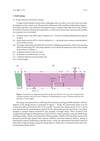
This document summarizes a study that used computational fluid dynamics (CFD) modeling and Taguchi-Grey relational analysis to optimize the design of flow control devices in a single-strand tundish. The study aimed to maximize the inclusion removal rate and minimize the dead volume fraction by optimizing the positions of the weir and dam. A Taguchi orthogonal array was used to analyze the effects of design factors on the responses. Grey relational analysis and analysis of variance were then used to determine the optimum positions of the weir and dam based on the multiple design targets of high inclusion removal rate and low dead volume fraction.

1. metals
Article
Design Optimization of a Single-Strand Tundish
Based on CFD-Taguchi-Grey Relational Analysis
Combined Method
Dong-Yuan Sheng 1,2
1 Department of Materials Science and Engineering, Royal Institute of Technology, 10044 Stockholm, Sweden;
shengdy@kth.se
2 Westinghouse Electric Sweden AB, 72163 Västerås, Sweden
Received: 18 October 2020; Accepted: 16 November 2020; Published: 19 November 2020
Abstract: A novel digital design methodology that combines computational fluid dynamics (CFD)
modelling and Taguchi-Grey relational analysis method was presented for a single-strand tundish.
The present study aimed at optimizing the flow control device in the tundish with an emphasis on
maximizing the inclusion removal rate and minimizing the dead volume fraction. A CFD model
was employed to calculate the fluid flow and the residence-time distribution of liquid steel in the
tundish. The Lagrangian approach was applied to investigate the behavior of non-metallic inclusions
in the system. The calculated residence-time distribution curves were used to analyze the dead
volume fraction in the tundish. A Taguchi orthogonal array L9(3ˆ4) was used to analyze the effects
of design factors on both single and multiple responses. Moreover, for the purpose of meeting
the multi-objective target functions, grey relational analysis and analysis of variance were used.
The optimum positions of the weir and the dam were obtained based on the design targets. A special
focus of this study was to demonstrate the capabilities of the Taguchi-Grey relational analysis method
as a powerful means of increasing the effectiveness of CFD simulation.
Keywords: clean steel; tundish; computational fluid dynamics (CFD); Taguchi; gray relational
analysis (GRA); digital design
1. Introduction
The tundish, working as a buffer and distributor of liquid steel between ladle and continuous
casting (CC) molds, plays a key role in affecting the performance of the CC machine, solidification of
liquid steel, quality, and productivity [1,2]. Tundish design varies widely from plant to plant, owing to
the differences in the end products, number of strands, and operating parameters. An optimum tundish
design aims at providing maximum opportunity for the control of liquid steel flow, heat transfer,
mixing, and inclusion removal. Considerable efforts have been made in both academia and industry
over many decades to fully exploit and enhance the metallurgical performance of the tundish [3,4].
Among this, computational fluid dynamics (CFD) and water model experiments have been considered
as useful and promising tools that can accurately predict many phenomena of practical interest in
tundish. A summary of the previous published modelling works can be found in the references [5,6].
The Taguchi method is a broadly accepted method of design of experiments (DOE), which has
been proven in producing high-quality products at subsequently low cost. It is considered to be
highly effective through following two aspects: (i) robust design—the approach of finding optimum
design factors that lead to economic designs with low variability; (ii) parameter design—the process
of identifying the settings of the design factors that reduce the design sensitivity due to the source
variation. Taguchi designs use orthogonal arrays to estimate the factors’ effect on the response mean
Metals 2020, 10, 1539; doi:10.3390/met10111539 www.mdpi.com/journal/metals

2. Metals 2020, 10, 1539 2 of 22
and variation. An orthogonal array means the design is balanced so that factor levels are equally
weighted. Thus, each factor can be assessed independent from the other factors. It reduces both time
and cost associated with the design trials when fractional factorial designs are used [7,8].
With the emphasis on superior steel quality, two indexes can be applied to evaluate the tundish
design: (i) inclusion remove rate (IRR); (ii) dead volume fraction (DVF). Dead zones can slowly mix
and contaminate the newly incoming steel. The inclusion removal rate is an index related to the steel
quality. The proper implementation of flow control devices (FCD) ensures the homogeneity of liquid
steel and enhances the inclusion removal. More specifically, it is necessary to obtain the optimum FCD
designs in tundish with high IRR and low DVF.
With focus on optimization of FCD design within the tundish, engineers have carried out a large
number of investigations using experimental and numeric approaches in order to address the relevant
design parameters that govern the desirable performance features. The literature on tundish design is
summarized in Table 1 [9–24]. The aforementioned studies have led to considerable improvements in
understanding various transport processes associated with tundish operations, aiming for the optimal
tundish design. However, few studies have employed a systematic approach to analyze how the
multiple design targets can be assessed simultaneously.
Normally, engineers can only simulate the process response through a one design factor at a
time strategy, while holding other parameters at a constant level. Thus, interaction effects between
dependent design factors are disregarded. Recently, attention has been drawn to systematic design
optimization with multiple design factors. This systematic approach is called design of experiments.
It allows explaining the interaction of design factors and the way the total system works by using
statistical analyses [25].
The objective of this study was to develop a digital design methodology that combined CFD
modelling and the Taguchi method for a single-strand tundish. A Taguchi orthogonal array L9(3ˆ4)
was used to analyze the effects of design parameters on both single (IRR, DVF) and multiple responses
(IRR + DVF). Grey relation analysis (GRA) was used for the multiple-response optimization. Analysis
of variance (ANOVA) was also carried out for finding out the contribution and impact of each design
factor towards the responses. The hydrodynamic modeling result allows to optimize flow control
device in the tundish with the emphasis on high IRR and low DVF. The optimum positions of the weir
and the dam were obtained based on the design targets. This study demonstrated that the digital
design, using the advanced computational methods, can be a significant technology for particles of
industrial design. Moreover, the digital design will become an important part for the digitalization
process in the steel industry.

3. Metals 2020, 10, 1539 3 of 22
Table 1. Summary of investigations modelling the optimum tundish design.
Reference Code Study 1
Strand 1 Turb. 2
Tundish Design
Case Method 3 FCD 4 Design Factors 5 Perform. Feature 6
Joo (1993) [9] METFLO n 2 k − ε 13 - D, W SFR, WAI, CFCD, WL, DL, FP, IRR
Craig (2001) [10] FLUENT n 1 k − ε 20 RSM TI, B, D, W, S WL, DL BL, BHA, FT FP, RTD
Jha(2004) [11] - N 6 (vari.) 6 - TI TM, OL, TIH, ID RTD
Hülstrung (2005) [12] - N 2 k − ε 10 - S, TI SFR, ID, IFR, CFCD V, IRR, RTD
Wei (2007) [13] - P 6 - 25 Taguchi B BD, HL RTD
Kumar (2008) [14] FLUENT N/P 2–6 k − ε 3 - D, TI CFCD V, RTD
Singh (2008) [15] FLUENT N/P 6 k − ε 6 - TI WAC, WAIA, TW V, WSS, RTD
Yang (2009) [16] FLUENT N/P/I 2 k − ε 5 - TI, IL, B, D DH, ILT
FP, RTD, V, WSS, T,
IRR, TO, TN
Cwudziński (2010) [17] FLUENT N/I 1 k − ε 12 - S, TI, D, GPB CFCD, GPBL, GFR FP, RTD
Tripathi (2012) [18] FLUENT N 1 k − ε 9 - ED EDL, MS V, RTD
Shukla (2013) [19] CFX N/P 1 k − ε - Taguchi D, W DH, DT, DL, WD, WT, WL, SFR RTD, IRR
Anapagaddi (2014) [20] CFX N 1 k − ε 7 RSM D, W IT, SFR, WL, WD, WT, DL, DH, DT RTD, IRR
Cloete (2015) [21] FLUENT N/P 4 k − ε 4 - TI, D CFCD, TIS, DH V, KE, RTD
He (2016) [22] FLUENT N/P 5 k − ε 3 - TI, B CFCD FS, V, T
Bul’ko (2018) [23] FLUENT N/P 2 k − ε 6 - TI TIS, SFR RTD, V
Sousa Rocha (2019) [24] CFX N/P 2 k − ε/SST 3 - D, W CFCD, ID RTD, IRR, FP, T
1 N: numerical model; P: physical model; I: industrial trials; 2 Turb.: turbulence model; vari.: turbulence model as variables; 3 Method.: Optimization or design method; RSM: response surface
models; 4 FCD: flow control devices; B: baffle; D: dam; ED: electromagnetic dam; GPB: gas permeable barrier; IL: inlet lauder; S: stopper; TI: turbulence inhibitor; W: weir; 5 BD: bath depth;
BL: baffle location; BHA: baffle hole angle; CFCD: combination of flow control devices; DL: dam location; DH: dam height; DT: dam thickness; EDL: electromagnetic dam location;
FT: fluid type; HL: hole location; IT: inlet temperature; ID: inlet depth; ILT: inlet lauder type; ID: inclusion diameter; IFR: inclusion flow rate; GPBL: gas permeable barrier location;
GFR: gas flow rate; MS: magnetic strength; OL: outlet location; SFR: steel flow rate; TM: Turbulence Model; TW: tundish width; TIS: turbulence inhibitor shape; TIH: turbulence inhibitor
height; WL: weir location; WD: weir depth; WT: weir thickness; WAC: wall curvature; WAI: wall inclination; WAIA: wall inclination angle; 6 Perform. Feature: performance feature;
FS: flow streamline; FP: flow pattern; IRR: inclusion removal rate; KE: kinetic energy RTD: residence time distribution parameter; T: temperature; TO: total oxygen measurement in steel
sample; TN: total nitrogen measurement in steel sample; V: velocity; WSS: wall shear stress.

4. Metals 2020, 10, 1539 4 of 22
2. Methodology
2.1. Design Objectives and Solution Strategy
A single-strand tundish (14 tons) with a submerged inlet, an outlet, a weir, and a dam was under
investigation in the current work. The geometric dimensions of the tundish are illustrated in Figure 1.
The liquid steel flow rate remained unchanged to keep a constant steel bath level in the tundish.
To maintain chemical and thermal homogeneity, as well as promote inclusion removal in the tundish,
two responses were considered:
(i) inclusion remove rate (IRR), which is defined as (1 − inclusions reaching outlet/inclusions injected
at inlet);
(ii) dead volume fraction (DVF), which is defined as (1 − calculated mean residence time/theoretical
mean residence time).
(iii) The design optimization should be able to meet the conflicting requirements, which are maximizing
IRR and minimizing DVF. The design objective was to obtain the optimized values of four design
factors (shown in Figure 1):
(iv) A (distance between inlet and weir),
(v) B (distance of tundish bottom to weir),
(vi) C (distance between weir and dam), and
(vii) D (dam height).
Metals 2020, 10, x FOR PEER REVIEW 4 of 21
2. Methodology
2.1. Design Objectives and Solution Strategy
A single-strand tundish (14 tons) with a submerged inlet, an outlet, a weir, and a dam was under
investigation in the current work. The geometric dimensions of the tundish are illustrated in Figure
1. The liquid steel flow rate remained unchanged to keep a constant steel bath level in the tundish.
To maintain chemical and thermal homogeneity, as well as promote inclusion removal in the tundish,
two responses were considered:
(i) inclusion remove rate (IRR), which is defined as (1 − inclusions reaching outlet/inclusions
injected at inlet);
(ii) dead volume fraction (DVF), which is defined as (1 − calculated mean residence time/theoretical
mean residence time).
(iii) The design optimization should be able to meet the conflicting requirements, which are
maximizing IRR and minimizing DVF. The design objective was to obtain the optimized values
of four design factors (shown in Figure 1):
(iv) A (distance between inlet and weir),
(v) B (distance of tundish bottom to weir),
(vi) C (distance between weir and dam), and
(vii) D (dam height).
Figure 1. Dimensions of a single-strand tundish: (a) side view (b) front view (unit: mm). Design
factors: A (distance between inlet and weir); B (distance of tundish bottom to weir); C (distance
between weir and dam); D (dam height).
The design was optimized by combining CFD simulation and Taguchi DOE methods. The flow
diagram of the design process is presented in Figure 2. Firstly, the optimization goals were set to
maximize IRR and minimize DVF in the tundish. Secondly, four design factors (A, B, C, and D) were
selected based on metallurgical expertise for the optimization process. Each factor was further
assigned a variation domain bounded by low, medium, and high values. These variations were
arranged through Taguchi orthogonal array (OA) L9(3^4) to create parametric computer-aided
design (CAD) geometries, which were utilized for CFD simulations. Thirdly, CFD simulation results
were post-processed through Taguchi data analysis, ANOVA, and Grey relational analysis, aiming
at selecting the optimal combination of design factors. Lastly, the optimization terminated when the
data-analyzed optimal design reached the design objective. Otherwise, it continued to loop with a
new set of proposed design factors.
Figure 1. Dimensions of a single-strand tundish: (a) side view (b) front view (unit: mm). Design factors:
A (distance between inlet and weir); B (distance of tundish bottom to weir); C (distance between weir
and dam); D (dam height).
The design was optimized by combining CFD simulation and Taguchi DOE methods. The flow
diagram of the design process is presented in Figure 2. Firstly, the optimization goals were set
to maximize IRR and minimize DVF in the tundish. Secondly, four design factors (A, B, C, and D)
were selected based on metallurgical expertise for the optimization process. Each factor was further
assigned a variation domain bounded by low, medium, and high values. These variations were
arranged through Taguchi orthogonal array (OA) L9(3ˆ4) to create parametric computer-aided design
(CAD) geometries, which were utilized for CFD simulations. Thirdly, CFD simulation results were
post-processed through Taguchi data analysis, ANOVA, and Grey relational analysis, aiming at
selecting the optimal combination of design factors. Lastly, the optimization terminated when the
data-analyzed optimal design reached the design objective. Otherwise, it continued to loop with a new
set of proposed design factors.

5. Metals 2020, 10, 1539 5 of 22
Metals 2020, 10, x FOR PEER REVIEW 5 of 21
Figure 2. Flow diagram of design process to optimize flow control device in tundish.
2.2. Design of Experiment
Minitab V.18 (Minitab, LLC, State College, Pennsylvania, PA, USA) software was used for DOE
analysis in this study [26]. The DOE consists of four phases: planning, characterization, optimization,
and verification. The multi-objective optimization was built by combining CFD simulation and
design of experiment.
2.2.1. Taguchi Design
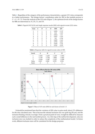
Taguchi analysis uses a classical signal-to-noise (S/N) ratio as a numerical measurement for
deciding the optimal circumstances. Noise (N) is the set of uncontrolled parameters that influences
the result or response. Signal (S) is the output variable or response. The S/N ratio indicates robustness
of an experiment. There are three categories of S/N ratios: (i) smaller-is-better, (ii) larger-is-better, and
(iii) nominal-is-best. The three S/N ratios are described in Equations (1)–(3). Depending on the
application, one should firstly identify the objective function to be optimized.
smaller-is-better: 2
1
1
/ 10log
n
i
i
S N y
n =
 
= −  
 
 
 (1)
larger-is-better: 2
1
1 1
/ 10log
n
i
i
S N
n y
=
 
= −  
 
 
 (2)
normal-is-best:
2
2
/ 10log
y
S N
s
 
 
=
 
 
(3)
where y is the performance characteristic value, n is the observation repeat number, and s2 is the
variance.
In this work, the Taguchi orthogonal array L9(3^4) was applied to define the optimum designs
regarding the selected factors. In Table 2, four factors with high, medium, and low values were
considered in DOE. As suggested by the Taguchi orthogonal array, nine CFD cases (cases 1–9) were
proposed with different combinations of the factor levels and displayed in Table 3. Case 0 (bare
tundish) was added as a reference case.
Figure 2. Flow diagram of design process to optimize flow control device in tundish.
2.2. Design of Experiment
Minitab V.18 (Minitab, LLC, State College, Pennsylvania, PA, USA) software was used for DOE
analysis in this study [26]. The DOE consists of four phases: planning, characterization, optimization,
and verification. The multi-objective optimization was built by combining CFD simulation and design
of experiment.
2.2.1. Taguchi Design
Taguchi analysis uses a classical signal-to-noise (S/N) ratio as a numerical measurement for
deciding the optimal circumstances. Noise (N) is the set of uncontrolled parameters that influences the
result or response. Signal (S) is the output variable or response. The S/N ratio indicates robustness of
an experiment. There are three categories of S/N ratios: (i) smaller-is-better, (ii) larger-is-better, and (iii)
nominal-is-best. The three S/N ratios are described in Equations (1)–(3). Depending on the application,
one should firstly identify the objective function to be optimized.
smaller-is-better : S/N = −10 log







1
n
n
X
i=1
y2
i






 (1)
larger-is-better : S/N = −10 log







1
n
n
X
i=1
1
y2
i






 (2)
normal-is-best : S/N = 10 log






y2
s2





 (3)
where y is the performance characteristic value, n is the observation repeat number, and s2 is the variance.
In this work, the Taguchi orthogonal array L9(3ˆ4) was applied to define the optimum designs
regarding the selected factors. In Table 2, four factors with high, medium, and low values were
considered in DOE. As suggested by the Taguchi orthogonal array, nine CFD cases (cases 1–9)
were proposed with different combinations of the factor levels and displayed in Table 3. Case 0
(bare tundish) was added as a reference case.

6. Metals 2020, 10, 1539 6 of 22
Table 2. Controlled factors and levels.
Factor Unit Level 1 Level 2 Level 3
A mm 640 840 1040
B mm 180 230 280
C mm 230 430 630
D mm 220 280 340
Table 3. Orthogonal array L9(3ˆ4).
Case A B C D
Case 0 - - - -
Case 1 1 1 1 1
Case 2 1 2 2 2
Case 3 1 3 3 3
Case 4 2 1 2 3
Case 5 2 2 3 1
Case 6 2 3 1 2
Case 7 3 1 3 2
Case 8 3 2 1 3
Case 9 3 3 2 1
2.2.2. Analysis of Variance
Analysis of variance (also referred to F-test) was developed by Ronald Fisher, the pioneer and
innovator of the use and application of statistical methods in experimental design [27]. The criteria
for determining the design factor’s effect on response function mainly rely on the magnitude of the
F-value, defined in Equation (4). The design factor with the highest F-value represents the factor with
the most significant effect on the response function.
F = MST/MSE (4)
where, MST is the mean square for treatments, and MSE is the mean square for error.
2.2.3. Grey Relational Analysis
Grey relational analysis (GRA), one of the most widely used models of Grey system theory, was
initially proposed by Deng [28]. GRA defines situations with no information as black and those with
perfect information as white. However, neither of these idealized situations occurs in real-world
problems. In fact, situations between these extremes, containing partial information, are described as
being grey. A variant of the GRA model, the Taguchi-based GRA model, is nowadays very popular in
engineering [29].
A multi-objective target is needed in the tundish design. To overcome the limitation of using
a single response by the Taguchi method, the GRA method [30] is here employed to convert the
multi-objective target into a single target optimization problem. The criteria of larger-is-better
and smaller-is-better have been used to describe the inclusion removal rate and the dead volume
fraction, respectively.
These factors are standard-transformed by Equations (5)–(7).
For the benefit-type factor : xi(k) =
xi(k) − minxi(k)
maxxi(k) − minxi(k)
(5)
For the defect-type factor : xi(k) =
maxxi(k) − xi(k)
maxxi(k) − minxi(k)
(6)

7. Metals 2020, 10, 1539 7 of 22
For the medium-type factor : xi(k) =
xi(k) − x0(k)
maxxi(k) − x0(k)
(7)
The grey relational grade (GRG) is calculated by the following steps:
(i) The absolute difference of the compared series and the referential series should be obtained by
Equation (8). The maximum and the minimum differences are obtained.
∆xi(k) = x0(k) − xi(k) (8)
(ii) Calculation of the relational coefficient and relational grade by Equation (9). The distinguishing
coefficient p is between 0 and 1. Typically, the distinguishing p value is set to be 0.5.
ξi(k) =
∆min + p∆max
∆xi(k) + p∆max
(9)
(iii) The grey relational grade is defined in Equation (10):
ri =
X
[w(k)ξ(k)] (10)
where ξ is the Grey relational coefficient, w(k) is the weight factor; w(k) is set as 0.5 in this study.
2.3. CFD Model
2.3.1. Model Description
CFD software STAR-CCM + V.13 (Siemens PLM software, Plano, TX, USA) was used to simulate
the fluid flow, the inclusion removal, and the residence-time distribution [31]. The assumptions made
for the mathematical model are described below:
• The model is based on a 3D standard set of the Navier–Stokes equations.
• Isothermal and steady-state liquid flow is considered.
• The motion of inclusions is simulated by solving the force balance equations.
• The realizable k-ε model is used to describe the turbulence.
• The free surface is flat and is kept at a fixed level. The tundish slag layer is not included.
• The surface tension and wettability at slag/steel/inclusion interphase boundaries are not included.
2.3.2. Governing Equations
The molten steel flow is defined as a three-dimensional flow with constant density. The calculation
of single-phase incompressible flow is accomplished by solving the mass and momentum conservation
equations. The equations solved in CFD code are written in a general form as
ρ
∂φ
∂t
+ ρuj
∂φ
∂xj
−
∂
∂xj





Γφ,ef f
∂φ
∂xj





 = Sφ (11)
where φ represents the solved variable, Γφ,eff is the effective diffusion coefficient, Sφ is the source term,
xj are the Cartesian coordinates, uj are the corresponding average velocity components, t is the time,
and ρ is the density. The first term expresses the rate of change of φ with respect to time, the second
term expresses the convection (transport due to fluid-flow), the third term expresses the diffusion
(transport due to the variation of φ from point to point), and the fourth term expresses the source terms
(associated with the creation or destruction of variable φ).

8. Metals 2020, 10, 1539 8 of 22
An Eulerian–Lagrangian approach was used to investigate the inclusion behavior in the tundish.
One-way coupling approach is considered, where the influence of the inclusion on the molten steel
flow is neglected. The transport equation for each inclusion particle is given as [31]
mi
dVp
∂t
= Fd + Fp + Fvm + Fg + Fl + Ftd (12)
where mi and Vp stand for the mass and velocity of a particle. On the right side of Equation (12),
the particle–fluid interaction forces are drag force (Fd), pressure gradient force (Fp), virtual mass forces
(Fvm), gravitational force (Fg), lift force (Fl), and turbulent dispersion (Ftd), respectively.
To calculate the residence-time distribution (RTD), a passive scalar transport equation is solved at
each time step [32,33].
ρ
∂C
∂t
+ ρuj
∂C
∂xj
−
∂
∂xj
Def f
∂C
∂xj
#
= 0 (13)
where the effective diffusivity, Deff, is the sum of the molecular and turbulent diffusivity. The velocity
field is solved obtained from a steady-state simulation and remained constant during the calculation of
the passive scalar.
In the tundish, the dead volume fraction was calculated with Equation (14):
Vd/Vt = 1 −
τ
τ
(14)
where τ is the calculated mean residence time, and τ is the theoretical mean residence time.
2.3.3. Numerical Modelling Details
The CFD mesh was generated using the trimmer and prism layer meshing options. Three prism
layers were generated next to all the walls. A reference mesh size of 0.006 m was used. The input
parameters for the CFD simulation are listed in Table 4. The surface average y + value is 2. The final
CFD model possesses a total of 2 million trimmer cells in the computing domain. The details of setting
up the CFD model and numerical solution procedure can be found in reference [6].
Table 4. Parameters and boundary conditions used for CFD simulations.
Parameter Value
Inlet velocity 1 m/s
Steel density 7020 kg/m3
Steel viscosity 0.006 Pa s
Reference pressure 101325 Pa
Inclusion velocity 1 m/s
Inclusion size 50 µm
Inclusion density 5000 kg/m3
Outlet (outflow ratio) 1
Wall No slip
Top surface Free slip
Tracer inlet (E-curve) 1 (t ≤ 0–2 s), 0 (t 2 s)
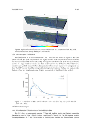
To simplify the model, those inclusion particles reaching the top surface and the outlet are regarded
as removal, while the rest are considered as rebound. In total, around 9500 inclusion particles are
injected through the inlet. Inclusion properties are listed in Table 4. It should be mentioned that
modelling the inclusion behavior is a task requiring comprehensive, multidisciplinary research. A large
number of particle interactions need to be considered in order to obtain the inclusion population
during the tundish casting process. As a first step of the modelling development, research work in this

9. Metals 2020, 10, 1539 9 of 22
paper was confined to describing only the simplified features of the inclusion removal. The growth
and collision mechanisms of inclusions were not considered.
3. Results
3.1. Validation of CFD Model
The CFD model was validated against the water model experiments reported in the literature by
Chen et al. [34]. The geometrical scale of the water model is 1:2. The experiment was carried out with
the dispersion of NaCl tracers. The pulse stimulus–response technique was employed to measure the
RTD E-curves. The NaCl solution was infused through the tracer inlet in 2 s. The change of tracer
concentration was registered continuously at the outlet.
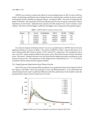
The RTD curves calculated from the CFD model are shown in Figure 3 along with the water
model results. The detailed input data for CFD calculations, including hydrodynamic parameters
and material properties, can be found in [34]. Figure 3 shows that the peak time in the bare tundish
(about 0.15 dimensionless time) was shorter than that in the gas curtain case (about 0.5 dimensionless
time). This indicates that in the bare tundish most liquid flowed directly to the outlet, leading to
a short residence time and large dead volume fraction. The gas curtain in tundish eliminated the
short-circuit flow, increased the residence time, and decreased the dead volume fraction. There is good
matching of the breakthrough time between the calculated and the measured results. The peak values
also agreed well with the experiment. The slopes of E-curves after the peak were close to each other.
Thus, the overall comparison between the simulation and the experiment is satisfactorily close.
Metals 2020, 10, x FOR PEER REVIEW 9 of 21
measure the RTD E-curves. The NaCl solution was infused through the tracer inlet in 2 s. The change
of tracer concentration was registered continuously at the outlet.
The RTD curves calculated from the CFD model are shown in Figure 3 along with the water
model results. The detailed input data for CFD calculations, including hydrodynamic parameters and
material properties, can be found in [34]. Figure 3 shows that the peak time in the bare tundish (about
0.15 dimensionless time) was shorter than that in the gas curtain case (about 0.5 dimensionless time).
This indicates that in the bare tundish most liquid flowed directly to the outlet, leading to a short
residence time and large dead volume fraction. The gas curtain in tundish eliminated the short-circuit
flow, increased the residence time, and decreased the dead volume fraction. There is good matching
of the breakthrough time between the calculated and the measured results. The peak values also
agreed well with the experiment. The slopes of E-curves after the peak were close to each other. Thus,
the overall comparison between the simulation and the experiment is satisfactorily close.
Figure 3. RTD curves of physical modelling and numerical modelling results (bare tundish and
tundish with gas curtain).
3.2. CFD Simulation Results
3.2.1. Fluid Flow
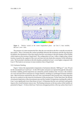
Figure 4 shows the predicted flow characteristics for Case 0 (bare tundish) and Case 1 (weir +
dam). The entering liquid jet flows down to the bottom of the tundish and spreads rapidly in the right
chamber. The flow is driven along the walls, then moves back to the entering jet. It forms counter
flows near the inlet region. A part of the incoming stream is confined within the region near the inlet
owing to the presence of the weir. Meanwhile, another part flow with high momentum moves
underneath the weir and downstream towards the outlet direction.
The presence of a dam reorients the flow after the weir and drives the flow vertically towards
the top surface. Thus, it increases the contact possibility between the inclusions and the top slag layer.
In addition, the interference of the dam impairs the flow recirculation in the left chamber of the
tundish, which improves the mixing of liquid steel. The configuration of Case 1 offers a higher plug
volume fraction caused by the support of the weir and dam and also limits the extension of the
turbulence zone. The horizontal velocities in the left chamber, predicted in Case 1, were higher
compared with Case 0. This leads to an increase in mean residence time of liquid steel.
Figure 3. RTD curves of physical modelling and numerical modelling results (bare tundish and tundish
with gas curtain).
3.2. CFD Simulation Results
3.2.1. Fluid Flow
Figure 4 shows the predicted flow characteristics for Case 0 (bare tundish) and Case 1 (weir + dam).
The entering liquid jet flows down to the bottom of the tundish and spreads rapidly in the right
chamber. The flow is driven along the walls, then moves back to the entering jet. It forms counter flows
near the inlet region. A part of the incoming stream is confined within the region near the inlet owing
to the presence of the weir. Meanwhile, another part flow with high momentum moves underneath
the weir and downstream towards the outlet direction.

10. Metals 2020, 10, 1539 10 of 22
Metals 2020, 10, x FOR PEER REVIEW 10 of 21
Figure 4. Velocity vectors at the center longitudinal plane: (a) Case 0, bare tundish; (b) Case 1, weir +
dam.
3.2.2. Inclusion Tracking
Figure 5 shows the representative trajectories of inclusions (density: 5000 kg·m−3, size: 50 μm) for
the simulated Case 0 and Case 1. In the CFD model, inclusions are injected through the inlet plane.
For better visibility, particle trajectories are colored by particle residence time. In Case 1, the existence
of a weir and dam drives inclusions to a longer distance, resulting in a prolonged inclusion retention
time. Most inclusions restricted by the weir were concentrated in the pouring area, indicating that
the weir is conducive to the removal of inclusions in the pouring area. At the same time, the density
of inclusion trajectories of the downstream area and the number of trajectories reaching the outlet in
Case 1 were significantly lower than those in Case 0. It illustrates that the weir and dam could greatly
improve the overall inclusion remove rate. The floating inclusions on the top surface of the tundish
are presented in Figure 5. It shows that Case 1 had more entrapped particles at the top surface than
Case 0.
Figure 5. Representative trajectories of inclusions in the tundish: (a) Case 0, bare tundish; (b) Case 1,
weir + dam (inclusion density: 5000 kg·m−3, size: 50 μm).
Figure 4. Velocity vectors at the center longitudinal plane: (a) Case 0, bare tundish;
(b) Case 1, weir + dam.
The presence of a dam reorients the flow after the weir and drives the flow vertically towards the
top surface. Thus, it increases the contact possibility between the inclusions and the top slag layer.
In addition, the interference of the dam impairs the flow recirculation in the left chamber of the tundish,
which improves the mixing of liquid steel. The configuration of Case 1 offers a higher plug volume
fraction caused by the support of the weir and dam and also limits the extension of the turbulence
zone. The horizontal velocities in the left chamber, predicted in Case 1, were higher compared with
Case 0. This leads to an increase in mean residence time of liquid steel.
3.2.2. Inclusion Tracking
Figure 5 shows the representative trajectories of inclusions (density: 5000 kg·m−3, size: 50 µm)
for the simulated Case 0 and Case 1. In the CFD model, inclusions are injected through the inlet plane.
For better visibility, particle trajectories are colored by particle residence time. In Case 1, the existence
of a weir and dam drives inclusions to a longer distance, resulting in a prolonged inclusion retention
time. Most inclusions restricted by the weir were concentrated in the pouring area, indicating that
the weir is conducive to the removal of inclusions in the pouring area. At the same time, the density
of inclusion trajectories of the downstream area and the number of trajectories reaching the outlet in
Case 1 were significantly lower than those in Case 0. It illustrates that the weir and dam could greatly
improve the overall inclusion remove rate. The floating inclusions on the top surface of the tundish are
presented in Figure 5. It shows that Case 1 had more entrapped particles at the top surface than Case 0.

11. Metals 2020, 10, 1539 11 of 22
the weir is conducive to the removal of inclusions in the pouring area. At the same time, the density
of inclusion trajectories of the downstream area and the number of trajectories reaching the outlet in
Case 1 were significantly lower than those in Case 0. It illustrates that the weir and dam could greatly
improve the overall inclusion remove rate. The floating inclusions on the top surface of the tundish
are presented in Figure 5. It shows that Case 1 had more entrapped particles at the top surface than
Case 0.
Figure 5. Representative trajectories of inclusions in the tundish: (a) Case 0, bare tundish; (b) Case 1,
weir + dam (inclusion density: 5000 kg·m−3, size: 50 μm).
Figure 5. Representative trajectories of inclusions in the tundish: (a) Case 0, bare tundish; (b) Case 1,
weir + dam (inclusion density: 5000 kg·m−3, size: 50 µm).
3.2.3. Residence-Time Distribution
The comparison of RTD curves between Case 1 and Case 0 is shown in Figure 6. For Case
0, bare tundish, the peak concentration was higher and the peak concentration time was shorter.
This means more tracer left the tundish quickly after injection into the tundish. Such flow characteristics
resulted in a large dead flow volume and short residence time. The RTD curve of Case 1 reveals a
smoother curve, which means the flow characteristics in Case 1 were improved by using a weir and
dam. The RTD curve in Case 0 has a long tail, indicating that a fraction of the fluid was retained in the
dead zone for a very long time, causing the poor homogeneity of liquid steel in the tundish.
Metals 2020, 10, x FOR PEER REVIEW 11 of 21
3.2.3. Residence-Time Distribution
The comparison of RTD curves between Case 1 and Case 0 is shown in Figure 6. For Case 0, bare
tundish, the peak concentration was higher and the peak concentration time was shorter. This means
more tracer left the tundish quickly after injection into the tundish. Such flow characteristics resulted
in a large dead flow volume and short residence time. The RTD curve of Case 1 reveals a smoother
curve, which means the flow characteristics in Case 1 were improved by using a weir and dam. The
RTD curve in Case 0 has a long tail, indicating that a fraction of the fluid was retained in the dead
zone for a very long time, causing the poor homogeneity of liquid steel in the tundish.
Figure 6. Comparison of RTD curves between Case 1 and Case 0 (Case 0, bare tundish; Case 1, weir +
dam).
3.3. Optimization Analysis
3.3.1. Single Response Optimization-Inclusion Remove Rate
The IRR values were calculated from the CFD particle tracking results, and their corresponding
S/N ratios are listed in Table 5. The IRR values varied from 74.7% to 87.6%. The IRR response table
for the design factors A, B, C, and D was created in the integrated manner, and the results are given
in Table 6. Regardless of the category of the performance characteristics, a greater S/N value
corresponds to a better performance. The design factors’ contribution order for IRR in the tundish
process is C A B D. From the analysis of the S/N ratio (Figure 7), the optimum levels of the design
factors for IRR are determined as A1, B1, C1, and D3.
Figure 6. Comparison of RTD curves between Case 1 and Case 0 (Case 0, bare tundish;
Case 1, weir + dam).
3.3. Optimization Analysis
3.3.1. Single Response Optimization-Inclusion Remove Rate
The IRR values were calculated from the CFD particle tracking results, and their corresponding
S/N ratios are listed in Table 5. The IRR values varied from 74.7% to 87.6%. The IRR response table for
the design factors A, B, C, and D was created in the integrated manner, and the results are given in

12. Metals 2020, 10, 1539 12 of 22
Table 6. Regardless of the category of the performance characteristics, a greater S/N value corresponds
to a better performance. The design factors’ contribution order for IRR in the tundish process is
C A B D. From the analysis of the S/N ratio (Figure 7), the optimum levels of the design factors
for IRR are determined as A1, B1, C1, and D3.
Table 5. Taguchi L9(3ˆ4) OA and single response results (IRR) with signal-to-noise (S/N) ratios.
Case A B C D IRR S/N
1 1 1 1 1 0.876 −1.15
2 1 2 2 2 0.81 −1.83
3 1 3 3 3 0.813 −1.8
4 2 1 2 3 0.827 −1.65
5 2 2 3 1 0.8 −1.94
6 2 3 1 2 0.829 −1.63
7 3 1 3 2 0.793 −2.01
8 3 2 1 3 0.839 −1.52
9 3 3 2 1 0.747 −2.53
Table 6. Response table for signal-to-noise ratios of IRR.
Level A B C D
1 −1.593 −1.605 −1.435 −1.874
2 −1.739 −1.764 −2005 −1.825
3 −2.024 −1.987 −1.917 −1.658
Delta 0.431 0.382 0.570 0.216
Rank 2 3 1 4
Metals 2020, 10, x FOR PEER REVIEW 12 of 21
7 3 1 3 2 0.793 −2.01
8 3 2 1 3 0.839 −1.52
9 3 3 2 1 0.747 −2.53
Table 6. Response table for signal-to-noise ratios of IRR.
Level A B C D
1 −1.593 −1.605 −1.435 −1.874
2 −1.739 −1.764 −2005 −1.825
3 −2.024 −1.987 −1.917 −1.658
Delta 0.431 0.382 0.570 0.216
Rank 2 3 1 4
Figure 7. Mean of S/N ratio (IRR) for each factor at levels 1–3.
ANOVA was chosen to analyze the effects of various design factors on IRR. It comes with two
merits: (1) obtaining contribution rate of design factors by analyzing the variation in factors, and (2)
verifying the results’ reliability by Taguchi analysis. As listed in Table 7, the term DF represents the
degree of freedom. The sequential (Seq SS) and adjusted (Adj SS) sums of squares indicate the relative
importance of each factor. Adjusted mean squares (Adj MS) measure how much variation a term
explains. The factor with the biggest coefficient and biggest sum of squares has the greatest impact.
To avoid zero degrees of freedom, factor D was set as a pooled factor in ANOVA due to its
lowest significant influence, as shown in Table 6. The results of ANOVA in Table 7 indicate that
factors A, B, and C influenced the IRR values by 24.64%, 19.18%, and 50.15%, respectively. The
contribution rate of error was 6.03%, which comprises different error parts, such as the external
sources and the calculation errors. The factor C (distance between weir and dam) had the highest
Figure 7. Mean of S/N ratio (IRR) for each factor at levels 1–3.
It should be mentioned here that the variation of IRR value is quite small, about 13% difference
for the nine calculated cases. This is because the selected inclusion size was quite big (50 µm), and the
inclusion floating velocity was high. From a practical point of view, it might be difficult to measure
such a small difference in the real tundish process. As a first step of the method development, only one
inclusion size was studied in order to reduce the complexity of the mathematical model. In future
work, different inclusion sizes will be considered for the design purposes.

13. Metals 2020, 10, 1539 13 of 22
ANOVA was chosen to analyze the effects of various design factors on IRR. It comes with two
merits: (1) obtaining contribution rate of design factors by analyzing the variation in factors, and (2)
verifying the results’ reliability by Taguchi analysis. As listed in Table 7, the term DF represents the
degree of freedom. The sequential (Seq SS) and adjusted (Adj SS) sums of squares indicate the relative
importance of each factor. Adjusted mean squares (Adj MS) measure how much variation a term
explains. The factor with the biggest coefficient and biggest sum of squares has the greatest impact.
Table 7. ANOVA table for inclusion removal rate.
Source DF Seq SS Contribution Adj SS Adj MS F-Value
A 2 0.002464 24.64% 0.002464 0.001232 4.09
B 2 0.001918 19.18% 0.001918 0.000959 3.18
C 2 0.005014 50.15% 0.005014 0.002507 8.32
Error 2 0.000603 6.03% 0.000603 0.000301 -
Total 8 0.009999 100.00% - - -
To avoid zero degrees of freedom, factor D was set as a pooled factor in ANOVA due to its lowest
significant influence, as shown in Table 6. The results of ANOVA in Table 7 indicate that factors A, B,
and C influenced the IRR values by 24.64%, 19.18%, and 50.15%, respectively. The contribution rate of
error was 6.03%, which comprises different error parts, such as the external sources and the calculation
errors. The factor C (distance between weir and dam) had the highest percentile contribution on the
inclusion removal rate. The significance of the design factors is determined as C A B, which is
consistent with the results from the Taguchi method.
3.3.2. Single Response Optimization-Dead Volume Fraction
Nine CFD cases of the transient RTD simulations were performed based on the Taguchi L9(3ˆ4)
OA. Figure 8 and Table 8 show the predicted E-curve and RTD parameters. It was found that the
selected design factors made a significant difference to the flow performance in the tundish, where the
predicted dead volume fraction varied from 9% to 26%.
Metals 2020, 10, x FOR PEER REVIEW 13 of 21
Error 2 0.000603 6.03% 0.000603 0.000301 -
Total 8 0.009999 100.00% - - -
3.3.2. Single Response Optimization-Dead Volume Fraction
Nine CFD cases of the transient RTD simulations were performed based on the Taguchi L9(3^4)
OA. Figure 8 and Table 8 show the predicted E-curve and RTD parameters. It was found that the
selected design factors made a significant difference to the flow performance in the tundish, where
the predicted dead volume fraction varied from 9% to 26%.
Figure 8. RTD curves of nine simulated cases based on Taguchi L9(3^4) OA.
Table 8. RTD analysis of nine simulated cases.
Case ttheo (s) tmin (s) tmax (s) tmean (s) Vd/V % Vp/V % Vm/V %
Case 0 742 100 251 629 15 24 61
Case 1 729 365 396 599 18 52 30
Case 2 729 92 165 591 19 18 63
Case 3 729 99 197 543 26 20 54
Case 4 729 95 382 584 20 33 47
Case 5 729 103 195 597 18 20 61
Case 6 729 224 452 603 17 46 36
Figure 8. RTD curves of nine simulated cases based on Taguchi L9(3ˆ4) OA.

14. Metals 2020, 10, 1539 14 of 22
Table 8. RTD analysis of nine simulated cases.
Case ttheo (s) tmin (s) tmax (s) tmean (s) Vd/V % Vp/V % Vm/V %
Case 0 742 100 251 629 15 24 61
Case 1 729 365 396 599 18 52 30
Case 2 729 92 165 591 19 18 63
Case 3 729 99 197 543 26 20 54
Case 4 729 95 382 584 20 33 47
Case 5 729 103 195 597 18 20 61
Case 6 729 224 452 603 17 46 36
Case 7 729 76 485 637 13 38 49
Case 8 729 134 338 588 19 32 48
Case 9 729 83 157 661 9 16 74
The DVF values calculated from the E-curves and their corresponding S/N ratio values are listed
in Table 9. The IRR response table for factors A, B, C, and D were created in an integrated manner,
and the results are given in Table 10. The optimal level of the DVF is the level with the greatest S/N
value. The order of importance of the design factors to the DVF is A D C B. From the analysis of
the S/N ratio (Figure 9), the optimum levels of the design factors for DVF are determined as A3, B3, C2,
and D1.
Table 9. Taguchi L9(3ˆ4) OA and S/N ratio of DVF (single response).
Case A B C D DVF S/N
1 1 1 1 1 0.179 14.933
2 1 2 2 2 0.190 14.447
3 1 3 3 3 0.255 11.869
4 2 1 2 3 0.199 14.033
5 2 2 3 1 0.182 14.796
6 2 3 1 2 0.174 15.195
7 3 1 3 2 0.126 17.966
8 3 2 1 3 0.194 14.230
9 3 3 2 1 0.094 20.579
Table 10. Response table for S/N ratios of DVF.
Level A B C D
1 13.75 15.64 14.79 16.77
2 14.67 14.49 16.35 15.87
3 17.59 15.88 14.88 13.38
Delta 3.84 1.39 1.57 3.39
Rank 1 4 3 2

15. Metals 2020, 10, 1539 15 of 22
Level A B C D
1 13.75 15.64 14.79 16.77
2 14.67 14.49 16.35 15.87
3 17.59 15.88 14.88 13.38
Delta 3.84 1.39 1.57 3.39
Rank 1 4 3 2
Figure 9. Mean of S/N ratio (DVF) for each factor at levels 1–3.
The results of ANOVA in Table 11 indicate that factors A, C. and D influenced the DVF values
by 45.82%, 7.52%, and 42.64%, respectively. The contribution rate of error was 4.02%. To avoid zero
degrees of freedom in the ANOVA analysis, factor B was set as a pooled factor due to the lowest
significant influence, as shown in Table 10. Factor A (distance between inlet and weir) had the highest
percentile contribution on the dead volume fraction in the tundish. The significance of the design
factors is determined as A D C, which is consistent with the results acquired from the Taguchi
method.
Table 11. ANOVA table for dead volume fraction.
Source DF Seq SS Contribution Adj SS Adj MS F-Value
A 2 0.007597 45.82% 0.007597 0.003798 11.39
C 2 0.001247 7.52% 0.001247 0.000623 1.87
D 2 0.007070 42.64% 0.007070 0.003535 10.60
Error 2 0.000667 4.02% 0.000667 0.000333 -
Total 8 0.016580 100.00% - - -
Figure 9. Mean of S/N ratio (DVF) for each factor at levels 1–3.
The results of ANOVA in Table 11 indicate that factors A, C and D influenced the DVF values by
45.82%, 7.52%, and 42.64%, respectively. The contribution rate of error was 4.02%. To avoid zero degrees
of freedom in the ANOVA analysis, factor B was set as a pooled factor due to the lowest significant
influence, as shown in Table 10. Factor A (distance between inlet and weir) had the highest percentile
contribution on the dead volume fraction in the tundish. The significance of the design factors is
determined as A D C, which is consistent with the results acquired from the Taguchi method.
Table 11. ANOVA table for dead volume fraction.
Source DF Seq SS Contribution Adj SS Adj MS F-Value
A 2 0.007597 45.82% 0.007597 0.003798 11.39
C 2 0.001247 7.52% 0.001247 0.000623 1.87
D 2 0.007070 42.64% 0.007070 0.003535 10.60
Error 2 0.000667 4.02% 0.000667 0.000333 -
Total 8 0.016580 100.00% - - -
3.3.3. Multiple Response Optimization Using the Grey Relational Grade
Data pre-processing by GRA was performed on the CFD simulation results of the responses
in Table 12, namely IRR and DVF. The multiple responses obtained were firstly normalized.
Subsequently, the deviation sequences were computed. Then, the grey relational coefficient (GRC)
for each value of the response was calculated. Finally, the average of the GRC was computed
to determine the grey relational grade (GRG). The overall evaluation of the multiple performance
characteristics was based on the GRG data. The grade with highest value was assigned the highest rank.

16. Metals 2020, 10, 1539 16 of 22
Table 12. Data processing of grey relational analysis.
Case A B C D IRR DVF
Normalization
Deviation
Sequence
Gray
Relational
Coefficient GRG Rank
IRR DVF IRR DVF IRR DVF
1 1 1 1 1 87.6 18 1.000 0.469 0.000 0.531 1.000 0.485 0.743 1
2 1 2 2 2 81.0 19 0.488 0.406 0.512 0.594 0.494 0.457 0.476 7
3 1 3 3 3 81.3 26 0.512 0.000 0.488 1.000 0.506 0.333 0.420 9
4 2 1 2 3 82.7 20 0.620 0.348 0.380 0.652 0.568 0.434 0.501 6
5 2 2 3 1 80.0 18 0.411 0.452 0.589 0.548 0.459 0.477 0.468 8
6 2 3 1 2 82.9 17 0.636 0.502 0.364 0.498 0.578 0.501 0.540 5
7 3 1 3 2 79.3 13 0.357 0.797 0.643 0.203 0.437 0.711 0.574 3
8 3 2 1 3 83.9 19 0.713 0.376 0.287 0.624 0.635 0.445 0.540 4
9 3 3 2 1 74.7 9 0.000 1.000 1.000 0.000 0.333 1.000 0.667 2
The GRG values and their corresponding S/N ratio values are listed in Table 13. The GRG response
table for factors A, B, C, and D were created in an integrated manner, and the results are given in
Table 14. The optimal level of the GRG is the level with the greatest S/N value. The order of importance
of the design factors to the GRG in the tundish process is D C B A. From the analysis of the S/N
ratio of GRG (Figure 10), the optimum levels of the design factors are determined as A3, B1, C1, and D1.
Table 13. Taguchi L9(3ˆ4) OA and S/N ratio of GRG (multiple responses).
Case A B C D GRG S/N
1 1 1 1 1 0.743 −2.585
2 1 2 2 2 0.476 −6.456
3 1 3 3 3 0.420 −7.543
4 2 1 2 3 0.501 −5.999
5 2 2 3 1 0.468 −6.594
6 2 3 1 2 0.540 −5.355
7 3 1 3 2 0.574 −4.821
8 3 2 1 3 0.540 −5.350
9 3 3 2 1 0.667 −3.522
Table 14. Response table for S/N ratios of GRG.
Level A B C D
1 −5.528 −4.468 −4.430 −4.234
2 −5.983 −6.133 −5.326 −5.544
3 −4.564 −5.473 −6.319 −6.297
Delta 1.419 1.665 1.890 2.064
Rank 4 3 2 1

17. Metals 2020, 10, 1539 17 of 22
Metals 2020, 10, x FOR PEER REVIEW 16 of 21
Figure 10. Mean of S/N ratio (GRG) for each factor at levels 1-3.
As listed in Table 15, the results of ANOVA indicate that factors C, D, and B influenced the GRG
by 26.13%, 36.48%, and 22.56%, respectively. Factor A was set as a pooled factor due to the lowest
significant influence, as shown in Table 14. The contribution rate of error was 14.83%, which was
quite large. This means that the pooled factor A had a relatively high contribution (shown in Figure
9). According to the ANOVA analysis, dam height had the highest percentile contribution on the
DVF. The significance of the design factors is determined as D C B, which is consistent with the
results acquired from the Taguchi method.
Table 15. ANOVA table for grey relational grade.
Source DF Seq SS Contribution Adj SS Adj MS F-Value
C 2 0.02171 26.13% 0.02171 0.010853 1.76
D 2 0.03030 36.48% 0.03030 0.015150 2.46
B 2 0.01874 22.56% 0.01874 0.009372 1.52
Error 2 0.01232 14.83% 0.01232 0.006160 -
Total 8 0.08307 100.00% - - -
3.4. Confirmation Tests
The purpose of the confirmation tests was to validate the conclusion drawn during the analysis
phase. A new CFD simulation case, Case 10, was created with the newest optimum levels of the
design factors for inclusion removal rate; it is the combination of A1, B1, C1, and D3, as suggested in
Section 3.3.1. According to the analysis from Section 3.3.2., the optimum levels of the control factors
for DVF consisted of A3, B3, C2 and D1, which was exactly the same as Case 9 in the Taguchi L9(3^4)
OA. In terms of gray relational grade, a new simulation case (Case 11) was created with the optimum
levels of the control factors. It combines A3, B1, C1, and D1 in the design based on the analysis in
Section 3.3.3.
Figure 11a gives the simulated IRR value of Case 10 and Case 11, as well as the nine cases from
Taguchi L9(3^4) array described in Table 4. The inclusion removal of proposed optimum case (Case
10) was about 1% higher than that of Case 1 (87.6%), which had the highest inclusion removal in
Taguchi OA. Furthermore, the simulated IRR (88.6%) of Case 10 was in good agreement with the
predicted IRR value (89.4%) through DOE analysis, as shown in Table 16. Thus, the optimum case of
IRR (Case 10) was verified. The suggested the optimum case of DVF from statistical analysis was also
Figure 10. Mean of S/N ratio (GRG) for each factor at levels 1-3.
As listed in Table 15, the results of ANOVA indicate that factors C, D, and B influenced the GRG
by 26.13%, 36.48%, and 22.56%, respectively. Factor A was set as a pooled factor due to the lowest
significant influence, as shown in Table 14. The contribution rate of error was 14.83%, which was quite
large. This means that the pooled factor A had a relatively high contribution (shown in Figure 9).
According to the ANOVA analysis, dam height had the highest percentile contribution on the DVF.
The significance of the design factors is determined as D C B, which is consistent with the results
acquired from the Taguchi method.
Table 15. ANOVA table for grey relational grade.
Source DF Seq SS Contribution Adj SS Adj MS F-Value
C 2 0.02171 26.13% 0.02171 0.010853 1.76
D 2 0.03030 36.48% 0.03030 0.015150 2.46
B 2 0.01874 22.56% 0.01874 0.009372 1.52
Error 2 0.01232 14.83% 0.01232 0.006160 -
Total 8 0.08307 100.00% - - -
3.4. Confirmation Tests
The purpose of the confirmation tests was to validate the conclusion drawn during the analysis
phase. A new CFD simulation case, Case 10, was created with the newest optimum levels of the
design factors for inclusion removal rate; it is the combination of A1, B1, C1, and D3, as suggested in
Section 3.3.1. According to the analysis from Section 3.3.2, the optimum levels of the control factors
for DVF consisted of A3, B3, C2 and D1, which was exactly the same as Case 9 in the Taguchi L9(3ˆ4)
OA. In terms of gray relational grade, a new simulation case (Case 11) was created with the optimum
levels of the control factors. It combines A3, B1, C1, and D1 in the design based on the analysis in
Section 3.3.3.
Figure 11a gives the simulated IRR value of Case 10 and Case 11, as well as the nine cases from
Taguchi L9(3ˆ4) array described in Table 4. The inclusion removal of proposed optimum case (Case 10)
was about 1% higher than that of Case 1 (87.6%), which had the highest inclusion removal in Taguchi
OA. Furthermore, the simulated IRR (88.6%) of Case 10 was in good agreement with the predicted IRR
value (89.4%) through DOE analysis, as shown in Table 16. Thus, the optimum case of IRR (Case 10)

18. Metals 2020, 10, 1539 18 of 22
was verified. The suggested the optimum case of DVF from statistical analysis was also Case 9 from
Taguchi OA. It had the best performance of dead volume fraction with 9.4%. It is interesting to observe
that Case 9 showed the best performance in minimizing dead volume, but behaved worst in removing
inclusion particles. This can infer that the two DVF and IRR responses in this study are in conflict with
each other. It is therefore of importance to develop a design optimization process considering multiple
responses simultaneously.
Metals 2020, 10, x FOR PEER REVIEW 17 of 21
Case 9 from Taguchi OA. It had the best performance of dead volume fraction with 9.4%. It is
interesting to observe that Case 9 showed the best performance in minimizing dead volume, but
behaved worst in removing inclusion particles. This can infer that the two DVF and IRR responses in
this study are in conflict with each other. It is therefore of importance to develop a design
optimization process considering multiple responses simultaneously.
Figure 11. Simulated IRR and DVF values by CFD: (a) IRR; (b) DVF.
Table 16. Results of confirmation tests.
Response Design Case CFD Prediction
IRR A1B1C1D3 10 88.6% 89.4%
DVF A3B3C2D1 9 9.4% 9.35%
GRG A3B1C1D1 11 0.798 0.790
Case 11- IRR: 86.8%; and DVF: 12.7% (CFD calculated)
The proposed optimum case of GRG, Case 11, is a compromised design with the concern of two
responses (IRR and DVF). Figure 12 gives the simulated GRG value of Case 11 together with the nine
cases from Taguchi OA described in Table 4. Case 11 showed the highest gray relational grade with
a value of 0.798. The design performance affirmed the validity of the Taguchi-GRA method for the
multi-response optimization of IRR and DVF. A good conformity was obtained by comparing the
simulated GRG value (0.798) by CFD and the predicted GRG value (0.79) by Taguchi-GRA, as shown
in Table 16.
Figure 12. Simulated GRG values by CFD.
Figure 11. Simulated IRR and DVF values by CFD: (a) IRR; (b) DVF.
Table 16. Results of confirmation tests.
Response Design Case CFD Prediction
IRR A1B1C1D3 10 88.6% 89.4%
DVF A3B3C2D1 9 9.4% 9.35%
GRG A3B1C1D1 11 0.798 0.790
Case 11- IRR: 86.8%; and DVF: 12.7% (CFD calculated)
The proposed optimum case of GRG, Case 11, is a compromised design with the concern of two
responses (IRR and DVF). Figure 12 gives the simulated GRG value of Case 11 together with the nine
cases from Taguchi OA described in Table 4. Case 11 showed the highest gray relational grade with
a value of 0.798. The design performance affirmed the validity of the Taguchi-GRA method for the
multi-response optimization of IRR and DVF. A good conformity was obtained by comparing the
simulated GRG value (0.798) by CFD and the predicted GRG value (0.79) by Taguchi-GRA, as shown in
Table 16.
Metals 2020, 10, x FOR PEER REVIEW 17 of 21
Case 9 from Taguchi OA. It had the best performance of dead volume fraction with 9.4%. It is
interesting to observe that Case 9 showed the best performance in minimizing dead volume, but
behaved worst in removing inclusion particles. This can infer that the two DVF and IRR responses in
this study are in conflict with each other. It is therefore of importance to develop a design
optimization process considering multiple responses simultaneously.
Figure 11. Simulated IRR and DVF values by CFD: (a) IRR; (b) DVF.
Table 16. Results of confirmation tests.
Response Design Case CFD Prediction
IRR A1B1C1D3 10 88.6% 89.4%
DVF A3B3C2D1 9 9.4% 9.35%
GRG A3B1C1D1 11 0.798 0.790
Case 11- IRR: 86.8%; and DVF: 12.7% (CFD calculated)
The proposed optimum case of GRG, Case 11, is a compromised design with the concern of two
responses (IRR and DVF). Figure 12 gives the simulated GRG value of Case 11 together with the nine
cases from Taguchi OA described in Table 4. Case 11 showed the highest gray relational grade with
a value of 0.798. The design performance affirmed the validity of the Taguchi-GRA method for the
multi-response optimization of IRR and DVF. A good conformity was obtained by comparing the
simulated GRG value (0.798) by CFD and the predicted GRG value (0.79) by Taguchi-GRA, as shown
in Table 16.
Figure 12. Simulated GRG values by CFD.
Figure 12. Simulated GRG values by CFD.

19. Metals 2020, 10, 1539 19 of 22
4. Summary and Conclusions
A novel digital design methodology that combined CFD simulation and Taguchi-Grey relational
analysis was presented with the aim of optimizing the design of flow control devices (weir and dam)
in a single-strand tundish. The design targets are set to maximize the inclusion removal rate and
minimize the dead volume fraction in the tundish. Four design factors were selected, including
distance between inlet and weir (A), distance of tundish bottom to weir (B), distance between weir
and dam (C), and dam height (D). From the CFD simulation results and the DOE analysis, the main
conclusions of this study can be drawn.
(1) The fluid pattern and the residence-time distribution were improved in the tundish furnished
with the weir and dam, in comparison with that in the bare tundish. The weir confined high
turbulent flow in the entry zone and increased the inclusion removal possibility by the top
surface. In addition, the dam drove the flow vertically towards the top surface and enhanced the
inclusion removal.
(2) With regard to the design optimization for the single response of IRR, the importance order of the
design factors was concluded as C A B D. The optimum levels of the control factors for IRR
were determined as the combination of A1, B1, C1, and D3. The reliability of the Taguchi analysis
results was verified by ANOVA.
(3) In terms of single response of DVF, the importance order of the design factors was considered
as A D C B. The optimum levels of the control factors for DVF were predicted as the
combination of A3, B3, C2, and D1. It was found that the optimum case of DVF had the best
performance in minimizing dead volume, but the worst performance in removing inclusion
particles. The conflicting responses suggests the necessity of developing a compromised
optimization process of multiple objectives. The evaluation of the multiple responses was
based on the grey relational grade. The importance order of the design factors for GRG is termed
as D C B A. The dam height was the most important factor affecting the GRG. The optimum
levels of the control factors were termed as the mixture of A3, B1, C1, and D1.
(4) The confirmation tests with regards to the different responses (IRR, DVF, and GRG) were performed.
The optimum results from CFD simulations revealed the increased performance of the responses.
An excellent agreement was observed between the CFD simulations and the DOE predictions.
(5) The present study demonstrated that the application of CFD combined with the Taguchi-GRA
method was effective in finding the optimal design that improved the tundish performance.
The developed method may provide both time and cost savings not only for researchers but also
for the steel industry. As shown in this study, a full design space (four design factors and three
levels) requires a total of 81 (3 × 3 × 3 × 3) computer runs. By applying the Taguchi orthogonal
arrays method, the computer runs can be significantly reduced to 9. Furthermore, the conclusions
drawn from small-scale experiments are valid over the entire experimental region spanned by the
design factors and their levels. Future work should test the applicability of the developed design
methodology in a wider range of experiment conditions.
Funding: This paper was supported by the Swedish Foundation for Strategic Research (SSF)—Strategic Mobility
Program (2019).
Acknowledgments: The author would like to acknowledge the Swedish Foundation for Strategic Research (SSF)
for their financial support via Strategic Mobility Program (2019).
Conflicts of Interest: The author declares no conflict of interest.
Nomenclature
Adj SS Adjusted sums of squares
Adj MS Adjusted mean squares
Deff Effective diffusivity
Fd Drag force

20. Metals 2020, 10, 1539 20 of 22
Fp Pressure gradient force
Fvm Virtual mass forces
Fg Gravitational force
Fl Lift force
Ftd Turbulent dispersion
g Gravity
Gk Turbulent kinetic energy
k Turbulent kinetic energy
mi Mass
n observation repeat number
SF Source term
s2 the variance
Seq SS Sequential sums of squares
u Velocity of the flow field
vl The velocity of liquid
vp The velocity of particle
Vp Velocity of particle i
υ Kinematic viscosity
xi(k) sequence for the ith experiment
x0(k) reference sequence
y performance characteristic value
ξ Grey relational coefficient
µ Molecular viscosity
µt Turbulent viscosity
ρ Density
w(k) weight factor of the number k influence
∆ deviation
Abbreviations
ANOV
A Analysis of Variance
CC Continuous Casting
CAD Computational Aided Design
CFD Computational Fluid Dynamics
DOE Design of Experiment
DVF Dead Volume Fraction
FCD Flow Control Device
GRA Grey Relational Analysis
GRC Grey Relational Coefficient
GRG Grey Relational Grade
IRR Inclusion Removal Rate
OA Orthogonal Array
RTD Residence-time distribution
S/N Signal-to-noise ratio
MST mean square for treatments
MSE mean square for error
References
1. Szekely, J.; Ilegbusi, O.J. The Physical and Mathematical Modeling of Tundish Operations; Springer Science and
Business Media LLC: New York, NY, USA, 1989.
2. Mazumdar, D.; Guthrie, R.I.L. The Physical and Mathematical Modelling of Continuous Casting Tundish
System. ISIJ Int. 1999, 39, 524–547. [CrossRef]
3. Chattopadhyay, K.; Isac, M.; Guthrie, R.I.L. Physical and Mathematical Modelling of Steelmaking Tundish
Operations: A Review of the Last Decade (1999–2009). ISIJ Int. 2010, 50, 331–348. [CrossRef]

21. Metals 2020, 10, 1539 21 of 22
4. Mazumdar, D. Review, Analysis, and Modeling of Continuous Casting Tundish Systems. Steel Res. Int.
2019, 90, 1800279. [CrossRef]
5. Sheng, D.-Y.; Yue, Q. Modeling of Fluid Flow and Residence-Time Distribution in a Five-strand Tundish.
Metals 2020, 10, 1084. [CrossRef]
6. Sheng, D.-Y. Mathematical Modelling of Multiphase Flow and Inclusion Behavior in a Single-Strand Tundish.
Metals 2020, 10, 1213. [CrossRef]
7. Taguchi, G.; Chowdhury, S.; Wu, Y. Taguchi’s Quality Engineering Handbook; John Wiley Sons Inc.:
Hoboken, NJ, USA, 2005.
8. Taguchi, G. Off-line and On-line Quality Control Systems. In Proceedings of the International Conference on
Quality Control, Tokyo, Japan, 17–20 October 1978.
9. Joo, S.; Han, J.W.; Guthrie, R.I.L. Inclusion behavior and heat-transfer phenomena in steelmaking tundish
operations: Part III. applications—Computational approach to tundish design. Met. Mater. Trans. A 1993, 24,
779–788. [CrossRef]
10. Craig, K.J.; De Kock, D.J.; Makgata, K.W.; De Wet, G.J. Mathematical Modeling of Iron and Steel Making
Processes. Design Optimization of a Single-strand Continuous Caster Tundish Using Residence Time
Distribution Data. ISIJ Int. 2001, 41, 1194–1200. [CrossRef]
11. Jha, P.K.; Dash, S.K. Employment of different turbulence models to the design of optimum steel flows in a
tundish. Int. J. Numer. Methods Heat Fluid Flow 2004, 14, 953–979. [CrossRef]
12. Hülstrung, J.; Zeimes, M.; Au, A.; Oppermann, W.; Radusch, G. Optimization of the Tundish Design to
Increase the Product Quality by means of Numerical Fluid Dynamics. Steel Res. Int. 2005, 76, 59–63.
[CrossRef]
13. Wei, Z.; Bao, Y.; Liu, J.; Gong, W.; Wang, B. Orthogonal analysis of water model study on the optimization of
flow control devices in a six-strand tundish. J. Univ. Sci. Technol. Beijing Miner. Met. Mater. 2007, 14, 118–124.
[CrossRef]
14. Kumar, A.; Mazumdar, D.; Koria, S.C. Modeling of Fluid Flow and Residence Time Distribution in a
Four-strand Tundish for Enhancing Inclusion Removal. ISIJ Int. 2008, 48, 38–47. [CrossRef]
15. Singh, V.; Pal, A.R.; Panigrahi, P. Numerical Simulation of Flow-induced Wall Shear Stress to Study a Curved
Shape Billet Caster Tundish Design. ISIJ Int. 2008, 48, 430–437. [CrossRef]
16. Yang, S.; Zhang, L.; Li, J.; Peaslee, K. Structure Optimization of Horizontal Continuous Casting Tundishes
Using Mathematical Modeling and Water Modeling. ISIJ Int. 2009, 49, 1551–1560. [CrossRef]
17. Cwudziñski, A. Numerical Simulation of Liquid Steel Flow in Wedge-type One-strand Slab Tundish with a
Subflux Turbulence Controller and an Argon Injection System. Steel Res. Int. 2010, 81, 123–131. [CrossRef]
18. Tripathi, A. Numerical Investigation of Electro-magnetic Flow Control Phenomenon in a Tundish. ISIJ Int.
2012, 52, 447–456. [CrossRef]
19. Shukla, R.; Anapagaddi, R.; Mangal, S.; Singh, A.K. Exploring the Design Space of a Continuous Casting
Tundish for Improved Inclusion Removal and Reduced Dead Volume. In Proceedings of the Science and
Technology of Ironmaking and Steelmaking, Jamshedpur, India, 16–18 December 2013.
20. Anapagaddi, R.; Shukla, R.; Goyal, S.; Singh, A. Exploration of the Design Space in Continuous Casting
Tundish. In Proceedings of the ASME 2014 International Design Engineering Technical Conference,
New York, NY, USA, 17–20 August 2014.
21. Cloete, J.; Akdogan, G.; Bradshaw, S.; Chibwe, D. Physical and numerical modelling of a four-strand
steelmaking tundish using flow analysis of different configurations. J. S. Afr. Inst. Min. Met. 2015, 115,
355–362. [CrossRef]
22. He, F.; Zhang, L.-Y.; Xu, Q.-Y. Optimization of flow control devices for a T-type five-strand billet caster
tundish: Water modeling and numerical simulation. China Foundry 2016, 13, 166–175. [CrossRef]
23. Bul’ko, B.; Priesol, I.; Demeter, P.; Gašparovič, P.; Baricová, D.; Hrubovčáková, M. Geometric Modification of
the Tundish Impact Point. Metals 2018, 8, 944. [CrossRef]
24. Rocha, J.R.D.S.; De Souza, E.E.B.; Marcondes, F.; De Castro, J.A. Modeling and computational simulation
of fluid flow, heat transfer and inclusions trajectories in a tundish of a steel continuous casting machine. J.
Mater. Res. Technol. 2019, 8, 4209–4220. [CrossRef]
25. Anthony, J. Design of Experiments for Engineers and Scientists; Elsevier: Amsterdam, The Netherlands, 2003.
26. Minitab 18 Statistical Software; Minitab, Inc.: State College, PA, USA, 2017. Available online: www.minitab.com
(accessed on 7 June 2017).

22. Metals 2020, 10, 1539 22 of 22
27. Fisher, R.A. Statistical Methods for Research Workers; Oliver Boyd: Edinburgh, UK, 1925.
28. Deng, J.-L. Control Problems of Grey Systems. Syst. Control Lett. 1982, 1, 288–294.
29. Wikipedia. Available online: https://en.wikipedia.org/wiki/Grey_relational_analysis
(accessed on 27 June 2020).
30. Yin, M.-S. Fifteen years of grey system theory research: A historical review and bibliometric analysis.
Expert Syst. Appl. 2013, 40, 2767–2775. [CrossRef]
31. Siemens. STAR-CCM + Version 13.04 User Guide; Siemens PLM Software: Munich, Germany, 2019.
32. Ghirelli, F.; Hermansson, S.; Thunman, H.; Leckner, B. Reactor residence time analysis with CFD.
Prog. Comput. Fluid Dyn. Int. J. 2006, 6, 241. [CrossRef]
33. Spalding, D. A note on mean residence-times in steady flows of arbitrary complexity. Chem. Eng. Sci. 1958, 9,
74–77. [CrossRef]
34. Chen, D.; Xie, X.; Long, M.; Zhang, M.; Zhang, L.; Liao, Q. Hydraulics and Mathematics Simulation on the
Weir and Gas Curtain in Tundish of Ultrathick Slab Continuous Casting. Met. Mater. Trans. A 2013, 45,
392–398. [CrossRef]
Publisher’s Note: MDPI stays neutral with regard to jurisdictional claims in published maps and institutional
affiliations.
© 2020 by the author. Licensee MDPI, Basel, Switzerland. This article is an open access
article distributed under the terms and conditions of the Creative Commons Attribution
(CC BY) license (http://creativecommons.org/licenses/by/4.0/).