SlideShare a Scribd company logo
1 of 118
Steel supply chain management
by simulation modelling
Maqsood Ahmad Sandhu
University of United Arab Emirates, Al-Ain, United Arab
Emirates, and
Petri Helo and Yohanes Kristianto
Logistic Research Group, University of Vaasa, Vaasa, Finland
Abstract
Purpose – The aim of this paper is to propose a simulation study
of the “steel supply chain” to
demonstrate the effect of inventory management and demand
variety on the bullwhip effect mitigation.
Design/methodology/approach – The relevant literature is
reviewed, and then the simulation
model proposed.
Findings – This study identifies reasons for sharing information
under varying levels of demand
and some variants, and demonstrates the benefits of mitigating
the bullwhip effect by applying a
design of experiment. It is shown that the information sharing is
able to mitigate the bullwhip effect in
the steel supply chain by extending the order interval and
minimising the order batch size.
Research limitations/implications – This study explores the
factors associated with the bullwhip
effect. This research is focused on built-to-order simulation, so
the results are only oriented on the basis of
orders; hence a simultaneous order- and forecast-based steel
supply chain should be carried out in the future.
Practical implications – This framework is expected to provide
a convenient way to measure the
optimum inventory level against a limited level of demand
uncertainty, and thus enterprises can
promote the supply chain coordination.
Originality/value – An innovative simulation model of the
“steel supply chain” is proposed, which
includes information sharing in the simulation model.
Furthermore, dynamic scheduling is shown by
applying a continuous ordering and order prioritization rule to
replace traditional scheduling methods.
Keywords Simulation, Modelling, Steel supply simulation,
Supply chain management
Paper type Research paper
1. Introduction
The pace of change and growing uncertainty about the way in
which markets will
evolve has made it increasingly important for companies to be
aware of supply chain
management (SCM). In general, SCM can be defined as a
process of integrating a chain
of entities (such as suppliers, manufacturers, warehouses, and
retailers) in a manner
which ensures the production and delivery of goods in the right
quantities and at the
right time, while minimising costs and satisfying customers.
The supply chain itself can be understood as a network of
autonomous
(or semi-autonomous) business entities involved in various
business activities which
produce and deliver, through upstream and downstream links,
goods and/or services
to customers. Lin and Shaw (1998) emphasised the notion of
value in seeing a supply chain
The current issue and full text archive of this journal is
available at
www.emeraldinsight.com/1463-5771.htm
The authors are most grateful to the anonymous referees for
their constructive and helpful
comments that helped to improve the presentation of the paper
considerably. Further, authors
are thankful to the European Union for funding this project:
SIMUSTEEL (optimization of stocks
management and production scheduling by simulation of
continuous casting, rolling and
finishing department). Contract No. RFSR-CT-2005-00046.
Steel supply
chain
management
45
Received 29 October 2010
Revised 2 May 2011
19 July 2011
Accepted 20 July 2011
Benchmarking: An International
Journal
Vol. 20 No. 1, 2013
pp. 45-61
q Emerald Group Publishing Limited
1463-5771
DOI 10.1108/14635771311299489
as a series of activities which delivers value to its customers, in
the form of a product or a
service (or a combination of the two), whereas Moon and Kim
(2005) emphasised the notion
of core flows, describing a supply chain in terms of flows (of
information, cash, and
materials) through a series of processes, beginning with
suppliers of raw materials and
finishing with the end customers.
If a supply chain is understood in the second sense (that is, in
terms of information
and material flows), a so-called “bullwhip effect” can occur
over time as the dynamics
of the flows change. The “bullwhip effect” is a phenomenon
whereby a small change in
demand among end customers is amplified as it progresses
upstream along the supply
chain. This has the potential to cause cycles of excess
inventory, severe backlogs,
inadequate product forecasts, unbalanced capacities, poor
customer service, uncertain
production plans, high backlog costs, and lost sales (Lee et al.,
1997; Zhang et al., 2004;
Law and Ngai, 2007; Hong et al., 2010).
The successful management of a supply chain is thus essentially
concerned with the
management of flows among entities, with a view to delivering
value. Indeed, Christopher
(1998) defined SCM as simply being the management of
upstream and downstream
relationships with suppliers and customers in such a way as to
deliver superior value to
customers at less cost to the supply chain as a whole. SCM thus
involves an integration
of various business processes. Many systems have been
developed in an attempt to
integrate business processes in various sectors of industry, for
example, enterprise
resource planning (ERP) is one such attempt to integrate several
data sources and
processes into a unified database system within an organisation.
By analogy, it might be
supposed that the integration of individual resource entities
within a supply chain could
provide overall integration of the supply chain itself. However,
resource planning of the
various organisational components that constitute a supply
chain is inherently likely to
be more demanding than a similar process within a single
organisation – simply because
resource planning would be need to be carried out
simultaneously within (and between)
all the entities in the supply chain.
There are many examples of business process improvement
through radical changes
(Hammer and Champy, 1993; Davenport, 1994; Levine, 2001;
Sandhu and Gunasekaran,
2004; Sandhu, 2005). However, there are also many reports of
the failure of attempts
to produce radical business process improvement – mainly due
to lack of tools for
evaluating the effectiveness of the designed solutions before
their implementation
(Tumay, 1996; Paolucci etal., 1997; Barber etal., 2003;
Greasley, 2003). There are also some
studies to improve supply chain process in the steel industry,
like Xiong and Helo (2008)
discuss supply chain and win-win path in visibility across all
participants, from steel
producers to customer demand. However, the benefits of
simulation modeling have been
ignored. In this regard, simulation modelling appears to have
great potential for analysing
business processes in a variety of industries (Hlupic and
Vreede, 2005). Simulation models
can incorporate the changing levels of such dynamic parameters
as demand variation,
production variation, arrival rates, and service intervals; these
can be used to
identify process bottlenecks and to assess suitable alternatives.
Simulation models can
also provide graphical displays of process models which can be
interactively edited
and animated to show the process dynamics of such phenomena
as the “bullwhip effect”.
Simulation has been applied to multi-agent supply chains to
investigate the dynamics
of the systems against sudden deviations in parameters, with a
view to optimising lead
times and minimising total costs (Swaminathan etal., 1998).
Similarly, Wilkner et al. (2007)
BIJ
20,1
46
used simulation to investigate order book effectiveness against
demand uncertainty,
and Towill (1996) studied the “bullwhip effect” by applying
control theory to inventory
and lead time minimisation. Our arguments are in line with Dale
(2001), who indicated
that simulation modelling has helped the aerospace industry.
Some guidelines for supply chain simulation have been
suggested for application in
the steel industry (Naylor et al., 2007; Dawande et al., 2004).
However, the authors focus
on production scheduling to minimise the on-hand inventory.
Other contributions, for
instance, Djamila (2003) add a multi-agent simulation into the
steel supply chain in order
to improve the design and performance of steel production and
scheduling. Hafeez et al.
(1996) use a system dynamic simulation to control the material
inventory. However,
fewer data are available on the use of information sharing by
means of simulation
analysis in the steel industry. Indeed, the failure to share
information tends to retain
greater inventory than is required for actual demand (Holweg
and Bicheno, 2002).
In view of this, the objective of the present study is to offer a
simulation tool which
management can use as a guide in determining inventory levels
and the “bullwhip
effect” at each level in the supply chain. The present study thus
extends previous theory
in SCM by using a simulation modelling approach to
demonstrate that the optimisation
of business processes needs to be complemented by
corresponding computer simulation
analysis. The research question guiding the study is:
RQ1. How does information sharing reduce the bullwhip effect?
The remainder of this paper is arranged as follows. Following
this introduction, the
next section reviews the literature on SCM, computer
simulation, steel supply chains,
and steel supply chain simulation. The following section
describes the proposed
simulation model. The paper then reports a simulation
experiment and its results.
Finally, the paper concludes with a discussion of the way in
which this simulation can
enhance the management of very varied demand. Future trends
and challenges in steel
supply chain simulation modelling are discussed and some
conclusions are drawn.
2. Theoretical background
2.1 Supply chain management
As noted above, a supply chain consists of several entities
(including customers,
distributors, manufacturers, and suppliers), each of which
contributes materials,
resources, and activities to the chain. To produce an optimal
result, managing a supply
chain thus requires integration of the entities at the structural
level and integration
of their individual systems. The benefits of effective SCM
include:
. Throughput improvements. Better coordination of materials
and capacity
prevents loss of utilisation while waiting for parts.
. Cycle time reduction. Consideration of constraints and
alternatives in the supply
chain helps to reduce cycle time.
. Inventory cost reductions. Knowledge of when to buy
materials (based on
accurate assessment of customer demand, logistics, and
capacity) reduces the
need for high inventory levels to guard against uncertainty.
. Optimised transportation. Effective SCM optimises logistics
and vehicle loads.
. Increased order fill rate. Real-time visibility across the supply
chain (alternate
routings, alternate capacity) enables order fill rates to be
increased.
Steel supply
chain
management
47
. Enhanced responsiveness to customers. Improved capacity to
deliver (based on
the availability of materials, capacity, and logistics) enhances
responsiveness to
customer needs.
In capital-intensive industries, such as steel-making, the
maintenance of a high utilisation
rate is a key success factor (Hill, 1994). However, the
scheduling problem in the steel
industry is acknowledged to be among the trickiest of several
industrial scheduling
problems (Lee and Murthy, 1996). The complexity lies in the
need to synchronise several
processes so as to create a flow through plants in which minimal
work in process is allowed
(Park et al., 2002). In these circumstances, improved scheduling
has the potential to create
significant economic gains. As Lee and Murthy (1996) put it:
In an industry where a single new manufacturing unit, such as a
continuous caster, can cost
more than $250 million, and where the annual production of the
unit is measured in hundreds
of millions of dollars, an expenditure in software development
to improve production even by
a few percent is worthwhile.
2.2 SCM simulation
Computer simulation has become a useful form of modelling in
many systems, including
economics, social sciences, manufacturing, and engineering.
Simulation typically uses a
mathematical model to predict the behaviour of the system from
a set of parameters and
initial conditions. The technique is often used for modelling
systems in which simple
closed-form analytical solutions are not possible. Although
there are different types of
computer simulation, the feature common to all is the
generation of a sample of
representative scenarios for a model in which the complete
enumeration of all possible
states of the model would be prohibitive or impossible.
The application of simulation in supply chains has tended to
emphasise a multi-agent
approach which takes account of the fact that supply chains are
composed of
autonomous or semi-autonomous agents (Swaminathan et al.,
1998). However, the main
issue in such multi-agent simulation is uncertainty regarding the
distribution of supply
chain activities among the various agents (Fox et al., 2000).
Simulation of a
decision-support environment for complex problem solving has
been used in the space
industry (Rabelo et al., 2006). Nevertheless, Fu et al. (2000) has
used such a
multi-agent simulation to enhance collaborative inventory
management and Towill and
Del Vecchio (1994) applied a similar technique with a view to
eliminating the “bullwhip
effect”. These studies suggest that multi-agent simulation
promises significant
improvement in SCM.
According to Chang and Makatsoris (2003), the benefits of
supply chain simulation
include:
. Improved understanding of the overall supply chain processes
and
characteristics by the provision of graphics/animation.
. Capturing of system dynamics through probability distribution
(including
the modelling of unexpected events in certain areas and their
impact on the
supply chain).
. Minimisation of the risk of changes in the planning process
through the
utilisation of what is called “what-if” simulation, which enables
the user to test
various alternatives before changing a plan.
BIJ
20,1
48
2.3 Steel supply chains and the “bullwhip effect”
Figure 1 shows the functions of a typical steel supply chain
from the mining of the iron
to the finished product. The present paper concentrates on the
“make-to-order” steps shown
in Figure 1 because the steps from iron mining to slab-casting
production (“make-to-stock”)
produce a homogeneous bulk product in a continuous production
process (rather than as
a series of discrete processes). The difference is significant. A
continuous process ensures
smooth production, whereas discrete processes are characterised
by numerous setups
and stock points, with an increased likelihood of overstocking
or stock-outs.
The “bullwhip effect” has long been a significant problem in
steel supply chains.
Possible solutions for reducing the effect were originally
proposed by Forrester (1961)
(based on a “DYNAMO” simulation model) and more recently
by Burbidge (1984) (based
on his shop-floor observations, supplemented by industrial
engineering analysis).
According to Forrester (1961), “bullwhip effects” can broadly
be identified as continuous
changes in the echelon time series with respect to demand,
orders, shipments, production,
and inventory. These “Forrester effects” generally exhibit long-
wavelength periodicity,
which can sometimes be related to the time delays in the
feedback paths used to correct
inventory discrepancies. According to Burbidge (1984),
“bullwhip effects” arise from
the batching of demand and production, and can therefore be
identified by discontinuous
(or sharp-edged) changes in the time series. These “Burbidge
effects” are generally
of shorter wavelength, although infrequent re-ordering or large
batch sizes can be
expected to produce longer wavelength fluctuations.
In the years since Forrester (1961) and Burbidge (1984)
proposed their ideas, research
into the “bullwhip effect” have been greatly extended and
further refined. McCullen and
Towill (2002) have claimed that variations in the steel supply
chain can be minimised,
but that it is important to identify the particular causes of
“bullwhip” in each instance.
Figure 1.
Functional structure
of steel supply chain
Steel supply
chain
management
49
Metters (1997) has built up a sophisticated model for estimating
the cost of “bullwhip”
using a form of dynamic programming which models the
optimum supply chain response
to a number of demand patterns. Towill’s et al. (2002) result is
an interesting one. He
shows that the Forrester effect causes the amplification of the
supply chain demand or
bullwhip effect. The interesting result is that this factor is
dependent of the information
confidence level of both supplier and buyer. Kelle and Milne
(1999) investigate how the
(s, S ) policy parameters, the demand parameters, and the cost
coefficients influence
the variability of the orders by using approximations to the
exact quantitative models.
It is shown that correlated demands can reduce demand
variability of aggregate orders
and smaller and more frequent order up to (OUT) policy can
reduce the order variability
and thus reduce the bullwhip effect. Partially, Cachon (1999)
supports the previous
contribution (Kelle and Milne, 1999) by suggesting a scheduled
ordering policy at smaller
batch size by taking risks of higher backorders and balanced
ordering policy where either
the supplier or the buyer may have different order interval to
minimize the buyer and the
supplier demand variances. Similarly, this present article use
information sharing where
either the buyer or the supplier will order if the current stock
below a certain level s and
fills the inventory by ordering the supplier as much as the
predicted future demand,
to represent balanced ordering policy. While Forrester (1961)
idea and the last two
contributions (Kelle and Milne, 1999; Cachon, 1999) are
contradictive one of another, it is
necessary to resolve the conflict by combining the balanced
ordering rule and longer
order interval without loosing the customer service level. In this
article, we use
information sharing to distribute the demand information to the
supplier and the buyer
and at the same time to give signal to them time to deliver.
Our model, furthermore use balanced supply to run OUT policy
based on the the
demand forecast. The demand forecast is centralized so as to
minimize the magnification
of customer demand information. Furthermore, we use
coefficient of variation (CV) as the
metric of the bullwhip effect to accommodate the effect of
demand correlation where the
bullwhip effect is measured by calculating the ratio of order
variance against OUT level.
The order interval is represented by using different level of
initial inventory where the
higher level of initial inventory signifies the longer ordering
interval and vice versa. The
performance measure of the ordering policy is the customer
service level.
The Bullwhip effect is also caused by price fluctuation from the
supplier that
motivates the buyer to order in larger quantities than the actual
customer demands
(Kaipia et al., 2002). However, Reiner and Fichtinger (2009)
model the effect of different
forecast model by including price effect. It is shown from the
case study of a two stage
supply chain with weekly empirical sales and pricing data that
different forecast model
might have different accuracy of predicting the future demand.
The reason is that
different forecast method has a difference level of
responsiveness against price
fluctuation that is defined as an offset of reference and observed
prices. It is also showed
that the forecast accuracy about customer demands is also
determined by the supply
chain responsiveness in terms of delivery response.
In considering the importance of demand forecast and supply
chain responsiveness
to mitigate the Bullwhip effect, Towill and Del Vecchio (1994)
use filter theory and
simulate this mechanism through a series of closed loop Fourier
analysis and first order
transfer functions from retailer to supplier. The adequacy of the
filter is determined by
the signal amplification from each echelon. Similar ideas are
also proposed by
Dejonckeere et al. (2000, 2002) who use automatic-pipeline,
inventory and order-based
BIJ
20,1
50
production control system (APIOBPCS) and Z-transform to
eliminate noise. It is clear
that demand information is smoothed, since no effort is made by
the supplier to
intervene in an order decision. Given this situation, without
assigning information
access to the supplier, it is possible to end up with a non-
optimum and trivial solution.
Second, information is batched and smoothed in an order book
before it is released to
a producer. For instance, in a work by Wilkner etal. (2007),
they used an order book with two
options. The first option was to maintain stability in the
delivery level by having flexible
production capacity. In contrast, the second option is to
maintain production stability by
letting demand fluctuate. The order book represents lists of
waiting orders which must be
fulfilled as promise. This paper makes no distinction between
standard modules and
customized modules and emphasizes analysis of ways to manage
a fixed customer order
decoupling point (CODP) and its influence in leading time
management issues. The CODP
concept in system dynamics is a gate between high variety and
smooth demand pattern
( Jones et al., 2000). It is clear that demand information is still
smoothed since efforts are
made to reduce manufacturers’ lead time. Hence, without
moving from make-to-forecast
to build-to-order, it is possible to end up with an unrealistic and
impractical solution.
Migrating from a make-to-forecast to a built-to-order is not a
winning strategy for
everyone. But all companies need to rigorously assess each of
their functions to
determine whether or not they have sufficient capacity to
perform this action. Greater
focus on synchronized supply can improve a company’s
strategic position by reducing
lead times, streamlining the inventory cost and improving
revenue. Finding optimum
lead times and inventory level usually allows companies to
enhance the core capabilities
that drive competitive advantage in their industries.
2.4 Simulation of SCM in the steel industry
Supply chain simulation to reduce the “bullwhip effect” has
been undertaken in the
automotive steel industry by Holweg and Bicheno (2002), who
used a lean processing
program applied to three tiers of the supply chain (slab-casting,
hot rolling mills (HRM), and
finishing coils) prior to component manufacture. The authors
investigated an
information-distortion effect to demand magnification in two
rounds of simulation. This
differed from the well-known “beer game” simulation in using a
“lean leap” logistics game –
because the “beer game” is not appropriate for application to a
manufacturing process that
consists of multiple stages and significant capacity constraints.
Holweg and Bicheno (2002)
concluded that synchronisation within the supply chain is
influenced by three factors:
(1) demand visibility;
(2) process visibility; and
(3) an appropriate time buffer.
Steel supply chain simulation has also been undertaken in the
context of business
strategy development by Hafeez et al. (1996), who analysed and
modelled two echelons
of a steel supply chain for the construction industry. The
authors adopted
a system-dynamics approach similar to that of Holweg and
Bicheno (2002) to minimise
lead times and inventory levels. Two kinds of model were
utilised:
(1) a conceptual model (to determine the dominant factors that
influence system
performance); and
(2) a quantitative model (representing a closed-loop system).
Steel supply
chain
management
51
The study, which used supply lead times as disturbance for the
modelled system,
produced a steel industry competitiveness index according to
various competitive
criteria. The authors concluded that this tool can serve as a
management information
system to measure competitiveness in the industry.
Supply chain simulation using a system-dynamics approach was
also developed
by Dawande et al. (2004), who used heuristic optimisation to
satisfy an order book. The
methodology involved the minimisation of slab inventory and
scrap, such that output was
in accordance with a targeted order weight. The authors
concluded that this heuristic
approach could be used to minimise slab “overweight” and cut
total costs significantly.
Steel supply chain simulation has also been used as an
educational tool in metallurgy
(Naylor et al., 2007). These authors developed an e-learning
facility which enabled students
to learn how to manufacture steel from an electric furnace to a
continuous casting run.
3. Developing a simulation model
Steel production is an extremely complex process and
determining coherent schedules
for the wide variety of production steps in a dynamic
environment, where disturbances
frequently occur, is a challenging task. In the steel production
process, the blast
furnace continuously produces liquid iron, which is transformed
into liquid steel in the
melt shop. Most of the molten steel passes through a continuous
caster to form large
steel slabs, which are rolled into coils in the hot strip mill.
The scheduling system of these processes has very different
objectives and constraints.
It operates in an environment where there is a substantial
quantity of real-time information
concerning production failures and customer requests. The
steel-making process, which
includes steel-making followed by continuous casting, is
generally the main bottleneck in
steel production. Therefore, comprehensive scheduling of this
process is critical for
improving the quality and productivity of the entire production
system.
Specific problem areas in steel production planning and
scheduling include inventory
management; slab, plate and cast design; and melting shop, hot
strip mill and finishing-line
scheduling. Optimizing each problem area independently can
result in savings for a steel
manufacturer. However, even greater gains can be achieved by
simultaneously optimizing
all of these interrelated areas. The combination of these
scheduling issues with the
instability of market conditions makes production planning in
the steel industry one of the
most challenging problems facing manufacturers today. Thus, a
central demand forecast
is proposed to support the production process in the supply
chain. The forecast is
distributed across the supply chain which minimises the
inventory investment. The
expected results are lower backorders and a lower inventory
level across the supply chain.
Figure 2, details the features of the simulation model, as
follows.
4. Simulation methodology
The research was funded by the European Union (EU) and was
investigated by the
research team at Slovakia and Finland. Simulation data
collection has been performed
in Košice, Slovakia and the process has included several
companies along the supply
chain. The research conducted contains model parts from the
mine, processing division
and production of iron (Fe) pellets, transport to the steel
manufacturing company,
reloading raw materials and storing inputs in materials stores
and Fe production in
three blast furnaces, Fe transport to the steel works, continued
casting works of the
slabs, repairing hall and storing in the cold store, modeling of
charging into the push
BIJ
20,1
52
furnaces, rolling on the wide hot rolling mill, and creating the
tin coils at the cutting
workshop. We define inputs and inputs as follows.
4.1 Inputs
Stock levels, varieties (sizes, length, thickness and width),
production time and its
standard deviation, transportation average delay, etc.
4.2 Output
Service level (percentage of on-time delivery), final inventory
levels and fill rate (the
number of completed orders per time unit, which can be
formulated as follows:
fill_rate ¼
Finished_coilðFCÞ_output
Completion_time
ð1Þ
Completion_rate ¼
Finished_coilðFCÞ_output
Demand
ð2Þ
In pursuit of these objectives, the simulated system took orders
from the order database,
and then prioritised them. Scheduled production was then
simulated and the outputs
were analysed. These outputs included inventory levels,
production throughput-time,
and customer satisfaction (proportion of orders produced on
time). Order batching was
used to represent economic production quantity, and the
simulation model was run
under three replications.
The model was able to generate production slips to the steel
factory, based on orders.
These orders were placed in a queue, and orders were fulfilled
according to priority.
The priority order was as follows:
Figure 2.
The three stage steel
supply chain model
Order
Type of
steel
Order
batching
Finishing
department
Slab
casting
Attribute
modifier
Attribute
modifier
HRM &
coiling
Finished
coil
inventory
coil
inventory
Slab
casting
inventory
Raw
material
Order
Delivery
Central forecast system
Delivery
Delivery
Stage 1 Stage 2 Stage 3
Steel supply
chain
management
53
. Stock of finished coils. If steel type and size matched from
shipment queue.
. Stock of coils. If steel type and thickness and width matched
or if it were possible
to cut ordered width size from coils of the finished department
queue.
. Stock of raw slabs. If steel type and order weight size matched
or if it were
possible to cut ordered weight size from slabs of furnace and
HSM queue.
. Raw material. If steel type did not match any stocks of
smelting queue.
The model was able to generate orders to raw material
suppliers, if:
(1) the actual inventory level of the raw material was below the
safety stock limit of
raw material orders; and
(2) there were backorders, where, after orders were matched
against available
stocks, the unfilled orders still remained in the orders queue.
4.3 System implementation
The specific problem areas in steel production planning (as
described above) were
simulated in a so-called “Simulsteel” model using Extend
simulation software
(Figure 2). The objectives of this simulation were:
(1) to identify the relationships between external factors (such
as variety of
customer demand) and internal factors (such as inventory
levels);
(2) to note the effects of these relationships on system
performance indicators (such
as final inventory level, order completion rate, and production
rate); and
(3) to investigate the influence of information sharing on
reducing the bullwhip effect.
Extend simulation software requires the assumption that the
model parameters and
model logic can be changed, making it easier to restate the
problems. The Extend simulation
models are constructed with library-based iconic blocks, which
each describe a calculation
or a step in a process. It is also possible to transfer the
simulation results into the Excel
worksheet for further analysis. Thus, the solution is connectable
and extendable to other
applications. Most importantly, the Extend software offers
visual transparency with no
programming necessary (Krahl, 2002).
The detailed steps of the simulation are introduced as follows:
(1) Demands arrive according to M/M/1 distribution and the
sales department
prioritize them according to their priority and stock availability.
Order scheduling
by prioritization is used by considering the process
commonality across the
entire factory. It is assumed that product varieties have different
processing times
and the highest priority is given to the one with the least
processing time.
Prioritization is done manually, using Microsoft Excel.
(2) In a simulation model with information sharing, customer
order is transmitted
directly to HRM department. This decision is taken in order to
short cut
information flow from finishing department to HRM department
and to reduce
inventory level in finishing department. Afterward, each stage
delivers the order
according to the demand information by considering the
delivery lead times and
the availability of stock in the downstream. In this model (s, S)
is not applied,
rather dynamic batch size is implemented to meet the customer
demands at
lower backorders and holding costs.
BIJ
20,1
54
(3) In addition to this production scheduling, an evolutionary
optimizer is applied
to optimize manufacturing time which consists of machining
time, holding time
in inventory and transportation time as it is formulated as
follows:
Max Profit ¼ Num Shipped*5000 2 Num Machines*100000
2 Num Holding Prods*10000 2 5000000=ðTransportTime
^2Þ
This optimization is operated separately from the simulation.
(4) The same processes are then followed by HRM and the slab-
casting
departments on the assumption that the processes are entirely
similar.
(5) To investigate the effect of information sharing, the
simulation model is then
modified by changing the order information path from the
finished coil
manufacturer directly to the hot rolling mill factory.
The above steps are then simulated by providing some inputs
and outputs to
investigate the performance of the supply chains. The choice of
input and output
parameters is made carefully to focus on the objective of this
simulation, that is, to
investigate the effect of inventory level on service level and the
effort of mitigating the
bullwhip effect.
5. Simulation results and analysis
Qualitative analysis is implemented to detect the existence of
the bullwhip effect. The
design of experiment (DOE) is used for making the analysis, by
considering the
following reasons:
. DOE is used to gather all information by considering process
variation, whether
or not it is under the full control of the experimenter.
. DOE is used to investigate the effect of intervention; some
objects, for instance,
demand variety and an inventory level up to the service level. In
this paper, we
wish to investigate whether both factors give co-intervention to
the experiment
outputs.
DOE is the only way to test the model when the variable is not
fully under control.
For example, the experimenter cannot assume that the beginning
inventory level and
demand variety as a fully non-correlated factor or, at the other
extreme, closely correlated.
Mathematical modelling in this case can replace DOE in
situations where the
experimenter knows exactly whether or not they are correlated.
Finally, DOE can be
summarized as follows:
Run number: 27.
Independent variables: demand, beginning inventory level.
Demand level: three levels (low (75), medium (100) and high
(125)).
Inventory level: three levels (low (60), medium (120) and high
(180)).
Replication number: 3.
Dependent variables: final inventory, completion rate and fill
rate.
Dependent variables: final inventory, completion rate and fill
rate.
Number of stages: three.
Steel supply
chain
management
55
In considering the limitation of the space, Table I exhibits an
example of Stage 1
simulation results. Next, similar operations are applied to Stage
2 and 3 (Table II).
5.1 Simulation model validation and verification
Table I is then analysed as performed in the ANOVA for
detecting the bullwhip effect
with a different level of demand and opening inventory. In the
first observation, Figure 3
shows the impact of inventory level on its variance. It is clear
that a high inventory level
gives no advantage because a company should put a higher
safety stock on this level.
The reason can be retrieved from Table III. The higher level of
inventory in Table III
indicates that the supply chain has no precise demand
information. This imprecision
in the information encourages the supply chain to install a
higher level of inventory.
Furthermore, it affects the fill rate (delivery) variation. This
combines imprecision in the
demand information with that on the delivery.
A similar DOE is also conducted to the supply chain with
information sharing
included and is benchmarked against the previous result, as
shown in Table III.
Table II shows the different performance levels between the
supply chain with and
without information sharing. It shows that the level of
production rate and fill rate
are two dependent variables affected by the demand and the
beginning inventory.
Input Output
Run Demand
Beginning
inventory
Final
inventory
Production
time
FC
output
Fill rate
(product/hour)
Completion
rate (%)
1 75 60 23 109 73 0.69 97
2 75 60 12 147 64 0.51 85
3 75 60 33 144 72 0.52 96
4 100 60 26 246 92 0.41 92
5 100 60 31 114 93 0.88 93
6 100 60 30 282 97 0.35 97
7 125 60 23 329 125 0.38 100
8 125 60 12 294 119 0.43 95
9 125 60 33 286 121 0.44 97
10 75 120 79 141 74 0.53 99
11 75 120 60 159 66 0.47 88
12 75 120 72 183 72 0.41 96
13 100 120 36 226 99 0.44 99
14 100 120 53 270 99 0.37 99
15 100 120 78 272 91 0.37 91
16 125 120 79 126 125 0.99 100
17 125 120 60 85 123 1.47 98
18 125 120 72 219 121 0.57 97
19 75 180 139 123 65 0.61 87
20 75 180 128 75 71 1.00 95
21 75 180 143 117 67 0.64 89
22 100 180 116 237 99 0.42 99
23 100 180 107 276 97 0.36 97
24 100 180 97 243 100 0.41 100
25 125 180 123 309 122 0.40 98
26 125 180 75 322 123 0.39 98
27 125 180 117 231 122 0.54 98
Table I.
Simulation results
BIJ
20,1
56
This implies that information sharing is capable of hedging the
adverse effect of the
variation in the demand by adjusting the fill rate and production
rate. Thus, balanced
ordering rule should be appropriate to the supply chain with
information sharing.
For providing information about the level of demand
magnification across the supply
chain, the bullwhip effect is measured. The bullwhip effect is
measured as the quotient of
the demand CV generated in a given supply chain level and the
demand CV received by that
same level (Fransoo and Wouters, 2000), since it explicitly
measures the relative variability
of order against demand as an explicit representation of the
bullwhip effect:
Figure 3.
Inventory variance as a
function of beginning
inventory level
Inventory variance
0
100
200
300
400
500
low medium high
Beginning inventory level
V
a
ri
a
n
c
e
Stage 1 Stage 2 Stage 3
With
information
sharing
Without
information
sharing
With
information
sharing
Without
information
sharing
With
information
sharing
Without
information
sharing
D ¼ 75 1.18 1.21 1.02 2.32 1 3.19
D ¼ 100 1.18 1.37 1.02 2.67 1 2.52
D ¼ 125 1.27 1.76 1.04 2.89 0.99 2.82
Table III.
Bullwhip effect of the
supply chain at different
demand levels
Without information sharing
With
information
sharing
Source Dependent variable F Sig. F Sig.
Demand Final inventory 2.229 0.136 1.561 0.532
Fill rate 2.086 0.153 6.032 0.028
Production rate 4.777 0.022 6.773 0.023
Beginning inventory Final inventory 100.155 0 0.956 2.867
Fill rate 0.822 0.456 0.998 1.439
Production rate 0.427 0.659 1.009 1.284
Demand * beginning inventory Final inventory 2.096 0.124
1.224 0.553
Fill rate 4.859 0.008 5.194 0.072
Production rate 0.773 0.557 5.386 0.018
Table II.
Tests of between-subjects
effects of Stage 1 in the
supply chain with and
without information
sharing
Steel supply
chain
management
57
BullwhipðBÞ ¼
sqnðtÞðt; t þ LdðnÞÞ=qnðtÞðt; t þ LdðnÞÞ
sDðtÞðt; t þ LdðnÞÞ=DðtÞðt; t þ LdðnÞÞ
¼
Rout
Rin
: ð3Þ
For sqn(t)(t,t þ Ld(n)) represents standard deviation during Ld,
the lead times of delivery,
qn(t)(t,t þ Ld(n)) represents the delivery rate according to the
demand at time t,
sD(t)(t,t þ Ld(n)) represents standard deviation demand during
the delivery lead time Ld
and D(t)(t,t þ Ld(n)) is the demand during the lead times.
Table III shows that the imprecision of the demand signal is
eliminated, such that
variation in the delivery lead times has no significant impact on
magnifying demand.
The EU, as the primary funder of this research, and the research
teams in Slovakia
and Finland verified the model through joint efforts between the
research team and
the case factory. The simulation was presented before both the
EU and the company
representatives. After undergoing some corrective actions,
finally the result was
acceptable.
6. Discussion
This experiment is intended to answer RQ1 about continuous
replenishment and the
effect of the inventory level on the order fulfilment rate
(product output rate and order
completion rate) and also the effect of information sharing on
mitigating the bullwhip
effect. Multivariate analysis of variance (MANOVA) is used in
order to assess the effect
of demand imprecision on the generation of the bullwhip effect.
The demand and the
beginning inventory level are used to indicate whether or not
the information of the
demand is imprecise. Thus, the final inventory level, the fill
rate (delivery rate) and
production rate are used as the performance indicators. Finally,
demand magnification
is measured through the quantification of the bullwhip effect.
Tables I and II reveal the information that enhancing the quality
of the demand
information gives some advantages. First, it reduces inventory
investment. Second,
it informs us that the demand variation has no effect on the
inventory investment,
however, different order interval affects on inventory
investment, with or without
information sharing. The longer order interval increases the
customer service level
as indicated in Table I. While the longer order interval increases
the service level,
however it also increases the requirement about safety stocks
(Figure 3). The result
support Cachon (2003) conclusion where the increasing of order
interval raises the
supply chain cost in terms of holding and backorder costs.
Furthermore, the longer
order interval reduces the fill rate of the supplier as a measure
of the batch size.
The combination of smaller batch size and longer order interval
could reduce the
Bullwhip effect (Kelle and Milne, 1999; Cachon, 1999).
The arrangement of the information flow has a significant effect
on order
completion at the agreed lead times. It is shown that allowing
HRM department as
supplier to access customer orders benefits the finishing
department in terms of order
completion rate. It implies that order amplification gives less
impact to a supply chain
which shares information. This result supports Dejonckeere et
al. (2000, 2002) in using
an APIOBPCS by providing information access to the supplier.
In conclusion, this simulation gives information to readers that
a high degree of
variety of demand should not cause a bullwhip effect as long as
such an order is
handled individually by a continuous replenishment policy and
information sharing.
As a consequence, a flexible production line should be
represented.
BIJ
20,1
58
7. Conclusion
This paper has considered information sharing in the steel
supply chain. The proposed
model has been successfully applied and has reduced the
Bullwhip effect and has
obtained related information on the production and fill rates.
Moreover, the adaptive
production and delivery rate are used to minimise the inventory
level. This study uses
a quotient of order and demand coefficient of variation, which
belong, respectively,
to Bullwhip measures and stock and delivery performance, in
order to compare the
performance of the supply chain with and without information
sharing. From observing
the results, it appears that the quality of demand information is
improved significantly
by providing a fill rate according to the demand and by reducing
the inventory
investment. Thus, the performances of the supply chain with
information sharing seems
to be better than its performances without information sharing
(Table III). In validating
the simulation model, we sent the report to the EU commission
for review. The EU
commission has approved the model with positive comments for
the implementation of
the results in the society. Further research may want to
investigate a number of
remaining issues. The steel supply chain must optimise the
responsiveness of the
production and delivery lead time to minimise the total supply
chain cost.
References
Barber, K., Dewhurst, F., Burns, R. and Rogers, J. (2003),
“Business-process modelling and
simulation for manufacturing management: a practical way
forward”, Business Process
Management Journal, Vol. 9 No. 4, pp. 527-42.
Burbidge, J.L. (1984), “Automated production control with a
simulation capability”, IFIP
Working Paper WG5(7), Copenhagen.
Cachon, G. (1999), “Managing supply chain demand variability
with scheduled ordering
policies”, Management Science, Vol. 45 No. 6, pp. 843-56.
Cachon, G.P. (2003), “Supply chain coordination with
contracts”, in de Kok, A.G. and
Graves, S.C. (Eds), Supply Chain Management: Design,
Coordination and Operation,
Elsevier, Amsterdam, pp. 229-340.
Chang, Y. and Makatsoris, H. (2003), “Supply chain modelling
using simulation”, International
Journal of Simulation, Vol. 2 No. 1, pp. 24-30.
Christopher, M. (1998), Logistics & Supply Chain Management,
2nd ed., Financial Times, London.
Dale, R. (2001), “Offline programming and simulation help
Boeing use giant automated riveter on
C-17 aircraft”, Industrial Robot: An International Journal, Vol.
18 No. 6, pp. 478-82.
Davenport, T. (1994), Process Innovation, Harvard Business
Press, Boston, MA.
Dawande, M., Kalagnanam, J., Lee, H.S., Reddy, C., Siegel, S.
and Trumbo, M. (2004), “The slab
design problem in steel industry”, INFORM, Vol. 34 No. 3, pp.
215-25.
Dejonckeere, J., Disney, S.M., Lambrecht, M.R. and Towill,
D.R. (2000), “Transfer function
analysis of forecasting induced bullwhip in supply chains”,
International Journal of
Production Economics, Vol. 78, pp. 133-44.
Dejonckeere, J., Disney, S.M., Lambrecht, M.R. and Towill,
D.R. (2002), “Measuring and avoiding
the bullwhip effect: a control theoretic approach”, European
Journal of Operational
Research, Vol. 147 No. 1, pp. 567-90.
Djamila, O. (2003), “A multi agent system for the integrated
dynamic scheduling of steel
production”, PhD thesis, University of Nottingham, School of
Computer Science and
Information Technology, Nottingham.
Steel supply
chain
management
59
Forrester, J. (1961), Industrial Dynamics, MIT Press,
Cambridge, MA.
Fox, M., Barbuceanu, M. and Teigen, R. (2000), “Agent
oriented supply chain management”,
The International Journal of Flexible Manufacturing System,
Vol. 12 No. 1, pp. 165-88.
Fransoo, J.C. and Wouters, M.J.F. (2000), “Measuring the
bullwhip effect in the supply chain”,
Supply Chain Management: An International Journal, Vol. 5 No.
2, pp. 78-89.
Fu, Y.H., Piplani, R., de Souza, R. and Wu, J. (2000), “Multi-
agent enabled modeling and
simulation towards collaborative inventory management in
supply chains”, Proceedings of
the 2000 Winter Simulation Conference, Vol. 2 No. 1, pp. 1763-
71.
Greasley, A. (2003), “Using business-process simulation within
a business-process reengineering
approach”, Business Process Management Journal, Vol. 9 No. 4,
pp. 408-21.
Hafeez, K., Griffiths, M., Griffiths, J. and Naim, M.M. (1996),
“System design of two echelon steel
industry supply chain”,
InternationalJournalofProductionEconomics, Vol. 45 No. 1, pp.
121-30.
Hammer, M. and Champy, J. (1993), Reengineering the
Corporation: A Manifest for Business
Revolution, HarperCollins Publisher, New York, NY.
Hill, T. (1994), Manufacturing Strategy – Text and Cases,
Palgrave, Basingstoke.
Hlupic, V. and Vreede, G.J. (2005), “Business process
modelling using discrete-event simulation:
current opportunities and future challenges”, International
Journal of Simulation and
Process Modeling, Vol. 1 Nos 1/2, pp. 72-81.
Holweg, M. and Bicheno, J. (2002), “Supply chain simulation –
a tool for education, enhancement
and endeavour”, International Journal of Production Economics,
Vol. 78 No. 1, pp. 163-75.
Hong, P., Dobrzykowski, D. and Vonderembse, M. (2010),
“Integration of supply chain IT and
lean practices for mass customization: benchmarking of product
and service focused
manufacturers”, Benchmarking: An International Journal, Vol.
17 No. 4, pp. 561-92.
Jones, R.M., Naylor, B. and Towill, D.R. (2000), “Engineering
the leagile supply chain”,
International Journal of Agile Management Systems, Vol. 2 No.
1, pp. 54-61.
Kelle, P. and Milne, A. (1999), “The effect of (s, S) ordering
policy on the supply chain”,
International Journal Production Economics, Vol. 59 Nos 1-3,
pp. 113-22.
Krahl, D. (2002), “The extended simulation environment”, in
Yücesan, E., Chen, C.-H., Snowdon, J.L.
and Charnes, J.M. (Eds), Proceedings of the 2002 Winter
Simulation Conference, pp. 205-13.
Law, C. and Ngai, E. (2007), “An investigation of the
relationships between organizational
factors, business process improvement, and ERP success”,
Benchmarking: An International
Journal, Vol. 14 No. 3, pp. 387-406.
Lee, H.L., Padmanabhan, V. and Whang, S. (1997), “The
bullwhip effect in the supply chain”,
Sloan Management Review, Spring, pp. 93-102.
Lee, H.S. and Murthy, S.S. (1996), “Primary production
scheduling at steel-making industries”,
IBM Journal of Research & Development, Vol. 40 No. 2, pp.
231-53.
Levine, L. (2001), “Integrating knowledge and processes in a
learning organization”, Information
System Management, Vol. 18 No. 1, pp. 21-32.
Lin, F. and Shaw, M.J. (1998), “Reengineering the order
fulfillment process in supply chain networks”,
International Journal of Flexible Manufacturing Systems, Vol.
10 No. 3, pp. 197-229.
McCullen, P. and Towill, D. (2002), “Diagnosis and reduction
of bullwhip in supply chains”,
International Journal of Supply Chain Management, Vol. 7 No.
3, pp. 164-79.
Metters, R. (1997), “Quantifying the bullwhip effect in supply
chains”, Journal of Operations
Management, Vol. 3 No. 15, pp. 89-100.
Moon, S.-A. and Kim, D.-J. (2005), “Systems thinking ability
for supply chain management”,
Supply Chain Management: An International Journal, Vol. 10
No. 5, pp. 394-401.
BIJ
20,1
60
Naylor, D.J., Bernhard, C., Green, A.M. and Sjökvist, T.
(2007), Learn How to Continuously Steel
on the Internet at Steeluniversity.org, available at:
http://library.mcc-cdl.at/8200.pdf
(accessed 12 February 2008).
Paolucci, E., Bonci, F. and Russi, V. (1997), “Redesigning
organisations through business
process re-engineering and object-orientation”, Proceedings of
the European Conference on
Information Systems, Cork, Ireland, pp. 587-601.
Park, H., Hong, Y. and Chang, S.Y. (2002), “An efficient
scheduling algorithm for the hot coil making
in the steel mini-mill”, Production Planning & Control, Vol. 13
No. 3, pp. 298-306.
Rabelo, L., Sepulveda, J., Compton, J. and Turner, R. (2006),
“Simulation of range safety for the
NASA space shuttle”, Aircraft Engineering & Aerospace
Technology: An International
Journal, Vol. 78 No. 2, pp. 98-106.
Reiner, G. and Fichtinger, J. (2009), “Demand forecasting for
supply processes in consideration of
pricing and market information”, International Journal of
Production Economics, Vol. 118
No. 1, pp. 55-62.
Sandhu, M. (2005), “Managing project business development:
an inter-organizational and
intra-organizational perspective”, doctoral dissertation, Swedish
School of Economics and
Business Administration, Helsinki.
Sandhu, M. and Gunasekaran, A. (2004), “Business process
development in project-based industry:
a case study”, Business Process Management Journal, Vol. 10
No. 6, pp. 673-90.
Swaminathan, J.R., Smith, S.F. and Sadeh, N.M. (1998),
“Modeling supply chain dynamics:
a multi agent approach”, Decision Sciences, Vol. 29 No. 3, pp.
607-32.
Towill, D.R. (1996), “Industrial dynamics modeling of supply
chains”, International Journal of
Physical Distribution and Logistics, Vol. 26 No. 2, pp. 23-42.
Towill, D.R. and Del Vecchio, A. (1994), “The application of
filter theory to the study of supply
chain dynamics”, Production Planning & Control, Vol. 5 No. 1,
pp. 82-96.
Towill, D.R., Childerhouse, P. and Disney, S.M. (2002),
“Integrating the automotive supply chain: where
are we now?”, International Journal of Physical Distribution &
Logistics Management, Vol. 32
No. 2, pp. 79-95.
Tumay, K. (1996), “Business process simulation”, Proceedings
of the 28th Conference on Winter
Simulation.
Wilkner, J.M., Naim, M. and Rudberg, M. (2007), “Exploiting
the order book for mass customized
manufacturing control systems with capacity limitation”, IEEE
Transactions on
Engineering Management, Vol. 54 No. 1, pp. 145-55.
Xiong, G. and Helo, P. (2008), “Challenges to the supply chain
in the steel industry”, International
Journal of Logistics Economics and Globalisation, Vol. 1 No. 2,
pp. 160-75.
Zhang, H., Li, H. and Tam, C. (2004), “Fuzzy discrete-event
simulation for modeling uncertain activity
duration”, Engineering, Construction and Architectural
Management, Vol. 11 No. 6, pp. 426-37.
Further reading
Hammer, M. (2007), “The process audit”, Harvard Business
Review, April.
Corresponding author
Maqsood Ahmad Sandhu can be contacted at: [email protected]
To purchase reprints of this article please e-mail:
[email protected]
Or visit our web site for further details:
www.emeraldinsight.com/reprints
Steel supply
chain
management
61
Reproduced with permission of the copyright owner. Further
reproduction prohibited without
permission.
IBM SPSS Step-by-Step Guide: t Tests
Note: This guide is an example of creating t test output in SPSS
with the grades.sav file. The variables shown in this guide do
not correspond with the actual variables assigned in Unit 8
Assignment 1. Carefully follow the Unit 8 Assignment 1
instructions for a list of assigned variables. Screen shots were
created with SPSS 21.0.
Assumptions of t Tests
To complete Section 2 of the DAA for Unit 8 Assignment 1, you
will generate SPSS output for a histogram, descriptive statistics,
and the Shapiro-Wilk test. (Levene test output will appear in
Section 4 of the DAA). Refer to the Unit 8 assignment
instructions for a list of assigned variables. The
examplevariables lowup and final are shown below.
Step 1. Open grades.sav in SPSS.
Step 2. Generate SPSS output for the Shapiro-Wilk test of
normality. (Refer to previous step-by-step guides for generating
histogram output and descriptives output for the Unit 8
assignment variables.)
· On the Analyze menu, point to Descriptive Statistics and click
Explore…
· In the Explore dialog box, move the assigned Unit 8 variables
into the Dependent List box. The final variable is used as an
example below.
· Click the Plots… button.
· In the Explore: Plots dialog box, select the Normality plots
with tests option.
· Click Continue and then OK.
Step 3. Copy the Tests of Normality table and paste it into
Section 2 of the DAA Template. Interpret the output.
Note: The Levene test is also generated as part of the SPSS t-
test output for Section 4 (discussed next). You do not have to
provide the Levene test output twice. You can report and
interpret it in Section 2 and then provide the actual output in
Section 4.
Reporting of t Tests
DAA Section 4 involves generating the t-test output and
interpreting it. The example variables of lowup (lower division
= 1; upper division = 2) and final are shown below.
Step 1. Generate SPSS output for the t test.
· On the Analyze menu, point to Compare Means and click
Independent-Samples T Test…
Step 2. In the Independent-Samples T Test dialog box:
· First, move the Unit 8 Assignment 1 dependent variable into
the Test Variable(s) box.
· Second, move the Unit 8 assignment variable into the
Grouping Variable box. Notice the (? ?) after the variable. The
values of the independent variable are assigned in the next step.
· Third, click the Define Groups… button.
· Fourth, in the Define Groups dialog box, assign the
corresponding values: Group 1 = 1, Group 2 = 2.
· Fifth, click Continue and then OK.
Step 3. Copy the output for the independent samples test and
paste it into Section 4 of the DAA Template. Then interpret it as
described in the Unit 8 assignment instructions.
2
Running head: DATA ANALYSIS AND APPLICATION
TEMPLATE
1
DATA ANALYSIS AND APPLICATION TEMPLATE
2Data Analysis and Application (DAA) Template
Name
University
Data Analysis and Application (DAA) Template
Use this file for all assignments that require the DAA Template.
Although the statistical tests will change from week to week,
the basic organization and structure of the DAA remains the
same. Update the title of the template. Remove this text and
provide a brief introduction.Section 1: Data File Description
1. Describe the context of the data set. You may cite your
previous description if the same data set is used from a previous
assignment.
2. Specify the variables used in this DAA and the scale of
measurement of each variable.
3. Specify sample size (N).
Section 2: Testing Assumptions
4. Articulate the assumptions of the statistical test.
5. Paste SPSS output that tests those assumptions and interpret
them. Properly integrate SPSS output where appropriate. Do not
string all output together at the beginning of the section.
6. Summarize whether or not the assumptions are met. If
assumptions are not met, discuss how to ameliorate violations
of the assumptions.Section 3: Research Question, Hypotheses,
and Alpha Level
1. Articulate a research question relevant to the statistical test.
2. Articulate the null hypothesis and alternative hypothesis.
3. Specify the alpha level.Section 4: Interpretation
1. Paste SPSS output for an inferential statistic. Properly
integrate SPSS output where appropriate. Do not string all
output together at the beginning of the section.
2. Report the test statistics.
3. Interpret statistical results against the null hypothesis.Section
5: Conclusion
1. State your conclusions.
2. Analyze strengths and limitations of the statistical
test.References
Provide references.
International Journal of Production Research
Vol. 50, No. 16, 15 August 2012, 4699–4717
Impact of the pull and push-pull policies on the performance of
a three-stage supply chain
Santosh Mahapatra*, Dennis Z. Yu and Farzad Mahmoodi
School of Business, Clarkson University, 311, Bertrand H. Snell
Hall, Potsdam, NY 13699, USA
(Received 4 January 2011; final version received 23 October
2011)
We investigate the performance of two common operating
policies (i.e., pull and push-pull) for a make-
to-stock product in an un-capacitated, three-stage supply chain.
The pull policy operates based on periodic
orders received from the immediate downstream facility.
However, in the push-pull policy, while processes
upstream of the order decoupling point are managed by the push
policy, the downstream processes are
managed by the pull policy. Simulation experiments are
conducted to examine the impact of each operating
policy under a variety of experimental conditions, characterised
by demand uncertainty and lead-time
variability. Our results indicate that the relative advantage of
the two policies is dependent on the type of
uncertainty, the level of uncertainty, the inventory control
policy and the performance measures of interest.
More specifically, while the push-pull policy results in lower
inventory, the pull policy yields a better fill rate.
This is in contrast to the notion that the pull policy generally
results in superior inventory performance.
Our findings suggest that firms should carefully consider the
level of uncertainty, the inventory control policy
and the performance measures of interest when determining the
operating policy.
Keywords: pull policy; push-pull policy; demand uncertainty;
lead-time variability; operational performance;
simulation research
1. Introduction
It is challenging to manage a multi-stage supply chain in an
environment characterised by uncertain customer
demand and variable manufacturing and distribution lead-times.
In such environments, the performance of a multi-
stage supply chain is manifested in terms of excess inventory,
poor customer service, or both. The push, pull and
push-pull (referred to as ‘hybrid’ here thereof) operating
policies are the three principal policies utilised to control
production and distribution systems (Karmarkar 1990). Whilst
in the push policy sourcing and production and
distribution processes are purely based on anticipated demand,
or forecast, in the pull policy such processes are
triggered after the customer order is received (Spearman and
Zazanis 1990). Alternatively, in the hybrid policy,
processes upstream of the order decoupling point (i.e. point of
differentiation) are managed by the push policy,
while the processes downstream of the order decoupling point
are managed by the pull policy (Pyke and
Cohen 1990).
While several studies have examined the push, pull or hybrid
policies in a single-stage supply chain, evaluation of
the policies in a multi-stage supply chain is rather limited and
the insights are either incomplete or case-specific
(see Masuchun et al. 2004). This can be attributed to a higher
level of operational challenges in multi-stage supply
chains than in single-stage chains. As such a comparative
assessment of the three policies is difficult because the
workings of the three policies are distinctly different, and the
criteria for evaluating the performance while
accounting for the difference in their workings are not clearly
outlined.
To address the knowledge gap, we investigate the performance
of two of the three policies (i.e. pull and hybrid
policies), while accounting for the basic tenets of the push and
pull-based operations. Our study involves a storable
product in a three-stage supply chain consisting of a
manufacturing plant, a warehouse and retailer(s). We do not
analyse the case when the push policy is implemented
throughout the supply chain. Such practice is fairly unrealistic
since in a typical multi-stage supply chain at least one of the
upstream facilities initiates production based on orders
from the downstream facilities. The operating policies are
carried out independently at the three facilities meaning
the information (e.g. forecasts or orders) that triggers actions is
generated locally. The decentralised characterisation
of the operations is consistent with the ‘push’ or ‘pull’
fundamentals (e.g. Pyke and Cohen 1990, Spearman and
*Corresponding author. Email: [email protected]
ISSN 0020–7543 print/ISSN 1366–588X online
� 2012 Taylor & Francis
http://dx.doi.org/10.1080/00207543.2011.637091
http://www.tandfonline.com
Zazanis 1990) and reflects the typical scenario of limited access
to information regarding other firms in a multi-stage
supply chain.
It is often conjectured by both practitioners and researchers that
performance of the pull policy is generally
superior to the push policy (Spearman and Zazanis 1990).
Although the hybrid policy combines the push and pull
policies, the conjecture regarding superior performance of the
pull policy does not hold as strongly when compared
with the hybrid policy. Previous studies have shown that the
performance of the pull and hybrid policies is affected
by demand uncertainty, forecast error and buffer stock levels
(e.g. Masuchun et al. 2004). However, these studies
have not systematically examined how lead-time uncertainty
and buffer stocks affect performance across the two
policies. In the extant studies, the inventory policies,
specifically the buffer stocks, have been chosen somewhat
arbitrarily. Consequently, the relative efficacy of the two
policies remains unclear.
We address these issues by examining the performance
dynamics under varied levels of demand uncertainty and
production/distribution lead-time variability when the buffer
stocks are chosen for a specified service level.
Specifically, our study intends to answer the following research
questions:
(1) How do demand and lead-time uncertainties affect the
performance of a three-stage supply chain?
(2) How do the performances of the pull and hybrid policies
differ in a three-stage supply chain?
We utilise simulation models in our analysis because the
simultaneous impact of multiple types of uncertainties
such as demand uncertainty, lead-time uncertainty and forecast
error is very difficult to examine analytically in a
multi-stage supply chain.
The remainder of the paper is organised as following. The
relevant literature is reviewed in the next section.
This is followed by a description of the supply chain structures
considered, simulation models and assumptions, as
well as the experimental design. Then, the simulation results for
a single retailer supply chain are discussed. This is
followed by a sensitivity analysis for a multiple retailer supply
chain. Finally, the conclusions and managerial
implications of the study are presented.
2. Literature review
Several studies have examined the effectiveness of the push,
pull and hybrid policies under a variety of operating
conditions; however, they differ significantly in the
implementation of the three policies. Since the push and pull
policies are fundamental to characterise the alternate policies, it
is useful to understand their distinctions. Pyke and
Cohen (1990) characterised the differences between the push
and pull policies in terms of production and order
quantity, timing of the production and shipment request, order
prioritisation rules and degree of managerial
interference. On the other hand, Bonney et al. (1999)
characterised the push and pull policies in terms of the flow of
control information. In a pull system the control information
flow typically is in the opposite direction of the
material flow. In contrast, the control information flow in a
push system is in the same direction as the material
flow. Furthermore, while in the pull system a downstream
facility with primarily local information exercises a
greater decision authority regarding the volume of supplies to
receive from the upstream facility, in the push system
the upstream facility with information that may be local or
global has a greater decision authority regarding the
volume of dispatch to the downstream facility (Pyke and Cohen
1990). Spearman and Zazanis (1990) noted that the
operating principles of the push and pull policies are radically
different. They observed that the push policy controls
operations in terms of production or distribution plan and
measures performance through work-in-progress (WIP)
inventory. In contrast, the pull policy controls operations in
terms of the level of WIP inventory and measures
performance in terms of the unmet demand.
Extant researchers have utilised analytical and simulation based
approaches to evaluate the performance of the
three alternate operating policies. While the analytical studies
(e.g. Spearman and Zazanis 1992, Pandey and
Khokhajaikiat 1996, Vidyarthi et al. 2009) utilised inventory
and queuing models to establish a functional
relationship between the various control variables in relatively
simple operating contexts, simulation studies
(e.g. Bonney et al. 1999, Maschun 1999, Li 2003, Maschun et
al. 2004) explored the interactions among a large
number of variables in relatively more complex operating
contexts. Most of the analytical studies have dealt with
either deterministic scenarios (e.g. Wang and Sarker 2006) or
stochastic analysis in relatively simple settings
(e.g. Spearman and Zazanis 1992, Pandey and Khokhajaikiat
1996).
Vidyarthi et al. (2009) utilised queuing theory to develop
analytical models to minimise response time while
optimally allocating workloads and creating capacity in make-
to-order and assemble-to-order supply chains.
4700 S. Mahapatra et al.
Their study did not analyse the performance of the push policy
for firm orders. Consequently, it provided limited
insights into the relative performance of the three policies.
Wang and Sarker (2006) proposed non-linear mixed
integer programming models for optimal Kanban-based control
of a manufacturer, warehouse and retailer supply
chain with deterministic demand and lead-time. The study
illustrated the usefulness of Kanban-based pull policy but
did not offer insights into its relative advantages over
alternative operating policies.
Pandey and Khokhajaikiat (1996) examined the performance of
the three alternate policies in a production
system that was modelled as a discrete time Markov process.
The system accounted for supply and production lead-
time uncertainty, demand uncertainty and raw material
constraints. They noted that no policy is distinctly superior
at all levels of demand uncertainty. While the performance of
the hybrid policy was generally superior, the push
policy (i.e. MRP based lot sizing) outperformed the hybrid
policy in the presence of raw material constraints. The
performance of the pull policy (i.e. Kanban based) was superior
only when the demand was very stable. Spearman
and Zazanis (1992) compared the performance of the push and
pull systems when processing time follows a Poisson
distribution, while demand is exponentially distributed. They
observed that the pull policy is easier to control and
performs better than the push policy because in the pull policy
the WIP inventory is bounded; however, the hybrid
policy (i.e. pull policy only at the final stage) can outperform
pure push and pull policies.
A few studies attempted to combine analytical approaches with
simulation approaches (e.g. Gonçalves et al.
2005, Su et al. 2010). In general, these studies formulated
models to describe the operations. The effectiveness of
these models was subsequently assessed using simulation. For
example, Gonçalves et al. (2005) formulated a model
for analysing the effect of demand uncertainty in a hybrid
system. Su et al. (2010) developed an M/M/1 base-stock
model to evaluate the effectiveness of delayed differentiation
when there are arrival and production variability in a
single-stage push system. Both studies utilised simulation to
obtain the performance results. It is apparent that it is
difficult to develop analytical models to compare the
performance of the three policies while capturing the
underlying details. Consequently, past studies (e.g. Spearman
and Zazanis 1992) have recommended simulation
studies to determine the effectiveness of alternate policies. In a
recent study, Almeder et al. (2009) observed that
analytical and simulation based researches should serve as
complements in studying supply chains.
In a typical supply chain, activities such as manufacturing,
warehousing and distribution have dissimilar task
complexities and lead-times, and are spatially and temporally
dispersed. These elements in combination affect the
supply chain performance; the combined impact of these factors
in a multi-stage supply chain has not been
examined adequately. In particular, most of the previous studies
(e.g. Closs et al. 1998, Grosfeld-Nir et al. 2000, Kim
et al. 2002, Li 2003, Masuchun et al. 2004, Teeravaraprug and
Stapholdecha 2004) do not examine how the supply
chain performance is affected by different levels of demand
uncertainty and lead-time variability.
The implementation and performance of the push, pull and
hybrid policies vary significantly from study to
study. In general, the studies differ in terms of the assumptions
regarding the inventory control policy, demand
uncertainty, lead-time variability, location of the order
decoupling point and knowledge of demand information
which affect the performance. Furthermore, most of the studies
do not explicitly account for forecast error, a key
determinant of the efficacy of push-based operations. Forecast
errors, usually include two components (i.e.
variability and bias), which have a significant impact on the
firm’s operational performance (Lee and Everett 1986,
Ritzman and King 1993). Forecast error is influenced by the
operational planning horizon, which is dependent upon
the operational lead-times and the frequency of plan updates.
The longer the planning horizon, the higher is the
forecast error (Chen et al., 2000). Based on a study of
population forecast errors, Smith and Sincich (1991)
concluded that there exists a linear or nearly linear relationship
between forecast inaccuracy and the length of the
forecast horizon. Therefore, it is useful to include these
considerations while accounting for the forecast errors.
As noted earlier, the existing studies are somewhat arbitrary in
their choice of the inventory policy. For example,
while some papers keep the same level of safety stocks for the
various policies to maintain comparability (e.g.
Pandey and Khokhajaikiat 1996, Closs et al. 1998), others
adjust the safety stocks arbitrarily with the change in
demand (e.g. Bonney et al. 1999, Masuchun et al. 2004). Most
of the studies have reported the snapshot
performance of the various operating policies (e.g. Closs et al.
1998), ignoring to reveal how the performance
changes over time. Prior studies have used a variety of
performance measures such as fill rate, throughput rate,
system inventory, retailer inventory, production lead-time,
inventory costs and the variability of fill rate. These
measures can be broadly classified into three categories: order
fulfilment rate, cycle time and inventory level.
Reporting of results in multiple forms presents difficulty in
comparing the performance.
To address some of the above shortcomings this study considers
the impact of forecast error, demand
uncertainty and lead-time variability on the inventory and fill
rate performance of the pull and hybrid policies. We
examine both longitudinal and snapshot results for the two
performance metrics. The experimental environment
International Journal of Production Research 4701
including the supply chain structures, simulation models,
assumptions as well as the experimental design are
discussed next.
3. Experimental environment
Our study considers a single-product supply chain with
geographically dispersed facilities. The supply chain consists
of a manufacturing plant, a warehouse and a retailer (or three
retailers in the multiple retailer system), and is
affected by varied levels of demand uncertainty and lead-time
variability. It is assumed that there is no capacity
constraint at any of the facilities. Labeling, packaging and
shipping operations are conducted in the warehouse. The
warehouse acts as a stocking point and supplies the retailer(s)
according to orders received from them. In the hybrid
policy, the warehouse receives supplies from the plant
according to demand forecasts at the plant; however, in the
pull policy, the warehouse receives supplies according to the
orders placed to the plant. Thus, the warehouse acts as
the order decoupling point in the hybrid policy. By assigning
the warehouse as the order decoupling point, we are
able to implement the pull operating policy to all or a part of
the supply chain. Two types of inventories (i.e. inputs
and outputs) are held at the plant and the warehouse. However,
only one type of inventory (finished goods) is held
at the retailer. The supply chain structures considered in the
study are depicted in Figure 1(a) and 1(b).
There are multiple lead-times in the supply chain: LT1 is
associated with the outside supplier (i.e. it takes LT1
days for the plant to receive a raw material order from the
supplier); LT2 is the production lead-time; LT3 is the
transportation lead-time between the plant and the warehouse;
LT4 is the warehouse assembling lead-time; and LT5
is the distribution lead-time between the warehouse and the
retailer(s).
Implementation of the push and pull policies can be carried out
in multiple ways (Pyke and Cohen 1990, Hopp
and Spearman 2004). In our model, the operations in the pull
policy at all upstream facilities are carried out based
on the replenishment orders from the immediate downstream
facility. The facilities review the inventory level (local
stock plus pipeline inventory) at the beginning of each week
and place an order to bring the inventory to the order-
up-to-level which is determined by the average demand during
the protection interval (the sum of the time period
between two successive reviews and the supply lead-time), plus
safety stocks to avoid shortage during the protection
interval. However, in the hybrid policy, while the operations at
the plant and dispatch to warehouse are governed by
the forecast requirements as in the push policy, the operations
and order fulfilments at the warehouse and the
retailer(s) are governed by actual orders as in the pull policy.
Thus, the plant develops the production plan based on
the customer demand forecasts and safety stock requirements,
without the knowledge of downstream inventory
levels. In the hybrid policy, the safety stocks for the push based
operations are maintained to avoid shortage during
the supply lead-times.
Pure forecast-based fulfilment from the plant to the warehouse
represents poor information flow between the
warehouse and the plant (Pyke and Cohen 1990). Note that such
unco-ordinated supply chains characterised by the
lack of cross-company integration and poor information flow
are observed in a variety of industries (Davis and
Spekman 2004). Figures 2 and 3 illustrate the operational
details of the pull and hybrid policies, respectively.
Plant
(b)
(a)
Warehouse
Supplier
Purchasing Production Assembly Distribution
LT1
LT4
LT3
LT2 LT5
Customer
Retailer
Plant Warehouse
Supplier
Purchasing Production Assembly Distribution
LT4
LT3
LT2
LT1
LT5
Customer
Customer
Customer
Retailer 1
Retailer 2
Retailer 3
Figure 1. (a) Supply chain structure: single retailer system; (b)
Supply chain structure: multiple retailer system.
4702 S. Mahapatra et al.
We assume that the supplier has enough capacity to fulfil all
orders from the plant. Nevertheless, raw material safety
stocks are held at the plant to cover for the demand and
supplier-to-plant transportation lead-time uncertainties.
The supplies from the plant and warehouse are constrained by
the available inventory. The unmet demands at the
plant and the warehouse are backlogged and manufactured with
a lag in the pull policy. However, in the
hybrid policy only the shortages of inputs that lead to
production shortfalls at the plant are backlogged
(refer to Figure 2). The input shortages at the warehouse and
output shortages at the plant are not backlogged
because the respective supplies occur based on push principles.
Accordingly, replenishment order for the input at the
plant is based on the forecast demand for week (t), the input
safety stock and the input shortage. At the retailer, if
there is insufficient inventory to satisfy the customer demand,
the unmet demand is lost without backordering
in both policies.
The supply chain structure allows postponement strategy in
packaging and shipping (i.e. operations that move
labelling processes such as language required, product stickers
and user manuals to the final phase of packaging).
Postponement processes produce generic products, which are
later customised upon receipt of an order. For
example, Hewlett-Packard has applied this strategy to packaging
and labelling of printers before shipping to
customers (www.kongandallan.com, 10 June 2007). Other
examples of the postponement strategy in packaging and
shipping include fast moving consumer goods companies that
sell a product under various brand names or in
various packaging sizes.
The principles for the push and pull policies in our study are
illustrated below in terms of production at the plant
and dispatch quantities to the warehouse.
Customer’s/retailer’s/warehouse’s
order arrives
Retailer/warehouse/plant
checks if available inventory can
satisfy the order?
Satisfy customer’s /retailer’s /
warehouse’s order and update
retailer’s/warehouse’s /plant’s
inventory status
Backlog any shortage at
warehouse /plant and
send available inventory
to retailer/warehouse
No
Yes
Calculating order -up-to level at
retailer/warehouse /plant according
to anticipated customer demand
during the protection interval
Retailer /warehouse /plant
checks if available inventory is
less than the order-up-to level?
Retailer/warehouse /plant orders
the difference between
inventory and order -up-to level
No action is needed
No
Yes
Figure 2. Illustration of the pull policy.
International Journal of Production Research 4703
Push policy: Production at the plant and dispatch quantities to
the warehouse:
Forecast requirement for week (t) from plant¼forecast demand
for week (t)þsafety stock at the warehouse
where,
safty stock ¼
ffiffiffiffiffiffiffiffiffiffiffiffiffiffiffiffiffiffiffiffiffiffiffiffiffiffi
ffiffiffiffiffiffiffiffi
½vaciance of weekly demand in week ðtÞ �avg: manuf: and
warehouse delivery
lead-time in weeks�þ ½squared avg: weekly demand in week
ðtÞ �variance of manuf: and
warehouse delivery lead-time in week�
z
vuuuuut
and
z standardised normal distribution statistic for the specified
service level
Production is carried out if and only if:
Output inventory at the plant in week (t)5 forecast requirement
for week (t)
Production at the plant for week (t)¼min [forecast requirement
for week (t), potential output
by the available input inventory in week (t)]
Shortages of inputs at plant in week (t)¼max [required inputs
for producing the forecast requirement
for week (t) – available input inventory in week (t), 0]
Dispatch to the warehouse for week (t)¼min [forecast
requirement for week (t), output inventory
at the plant in week (t)]
Pull policy: order to the plant and dispatch to the warehouse
Warehouse’s (input) order-up-to-level while reviewing for week
(t)
¼average demand during the protection intervalþsafety stock at
the warehouse
where,
safety stock ¼
ffiffiffiffiffiffiffiffiffiffiffiffiffiffiffiffiffiffiffiffiffiffiffiffiffiffi
ffiffiffiffiffiffiffiffiffiffi
variance of weekly demand in week ðtÞ �
avg. manuf. and warehouse delivery
lead-time in weeksþ review period in weeks
� �� �
þ½squared avg. weekly demand in week ðtÞ �variance of
manuf. and warehouse delivery
lead-time in weeks]
z
vuuuuuut
Customer demand
forecasts at plant for week t
Enough output
inventory at plant?
Calculation of required
output at plant
Calculation of required
input at plant accounting
for shortage
No
Yes
Dispatch available output to
warehouse and produce
required output at plant and
update inventory status
Sourcing raw
material if necessary
Dispatch required output
to warehouse and update
inventory status
Customer’s/retailer’s
order arrives
Retailer/warehouse
checks if available inventory
can satisfy the order?
Satisfy customer’s/retailer’s
order and update retailer’s/
warehouse’s inventory status
Backlog any shortage at
warehouse and send
available inventory to
retailer
No
Yes
Calculating order-up-to level at
retailer/warehouse according to
anticipated customer demand
during the protection interval
Retailer/warehouse checks
if available inventory is less than
the order-up-to level?
Retailer orders/warehouse
assembles the difference between
inventory and order-up-to level
No action is needed
No
Yes
Figure 3. Illustration of the hybrid policy.
4704 S. Mahapatra et al.
Replenishment order is placed to the plant if and only if:
(input) inventory at the warehouse in week (t) 5 order-up-to-
level for week (t)
Order quantity to the plant for week (t)¼max [order-up-to-level
for week (t) – (input) inventory at
the warehouse in week (t)þshortages of inputs in week (t), 0]
Where, shortages of inputs in week (t)¼min [0, (input)
inventory at the warehouse
in week (t) – warehouse output’s order quantity for week (t)]
Input inventory at the warehouse includes the inventory in
transit between the plant and the warehouse.
Dispatch to the warehouse for week (t)¼min [warehouse’s order
to the plant for week (t),
available inventory at the plant in week (t)]
Next, we describe the functional forms for demand and forecast
that are used to generate safety stocks, and
production and dispatch requirements. We adopt the following
demand function from Zhao et al. (2002) to generate
the customer demand at the retailer. The weekly demand
function is given by the following equation:
Demandt ¼ baseþ slope� tþ season� sin
2�
SeasonCycle
� t
� �
þnoise� snormal ðÞ ð1Þ
where, Demandt is defined as the demand in week t, snormal()
represents the standard normal distributed random
number generator, and SeasonCycle represents the weekly
demand effects (set to four in this study). The parameters
base, slope, season and noise characterise the level, growth,
seasonality and variability of the demand process,
respectively. The noise is expressed as a percentage of the base
demand. During the simulation, the average demand
for a specific week t is given by the first three terms of the
demand function. The standard deviation of demand for
computing safety stocks is calculated by the product of the
average demand and the coefficient of variation which is
generated according to the demand samples of Equation (1). We
utilise the above demand function because it is
comprehensive and includes the key elements that typically
characterise the demand in practice.
In the push policy, the demand forecast for week t, Forecast ,
made in week t0 for (t�t0) is generated by the
following equation (Zhao et al. 2002):
Forecastt ¼ Demandt �f1þEBþED�½1þðt� t0Þ=4:85��
snormal ð Þg ð2Þ
Forecasti has two components: customer demand during week
(t) and a forecast error coefficient which consists
of three components. The three components of forecast error
term are: the bias (EB), the variability (ED) which is
normally distributed, and a parameter (i.e. 1/4.85) representing
the rate of linear increase in ED with time to account
for higher forecast error for higher forecast horizon (e.g. t �
t0).
The forecast accuracy, forecast horizon, expected lead-times
and targeted service level are maintained as control
variables. The forecast horizons for procurement and production
at the plant are 7 and 6 weeks, respectively. Note
that the forecast horizon at the plant is longer than the average
supplier procurement and production lead-time.
This is consistent with the practice at many firms that utilise a
longer forecast horizon than the actual transportation
and manufacturing lead-time to account for developing the
forecast, communicating with the supplier or internal
divisions, arranging for resources, etc. that are extraneous to the
operations considered in our analysis.
We examine the performance implications through a series of
experiments. In our experiments, we consider three
levels of lead-time variability (i.e. LT standard deviation), as
well as three levels of demand uncertainty (i.e. noise).
The lead-time variability is assumed to be normally distributed
(Bowersox et al. 2002). We vary the manufacturing
lead-time variability at the plant, the transit lead-time
variability between the plant and the warehouse and the
transit lead-time variability between the warehouse and the
retailer. However, we do not vary the variability of
supplier lead-time because in a typical supply chain, contracts
are often executed to ensure timely supplier delivery
and the manufacturer can hold the supplier responsible for poor
delivery performance. We also do not vary the
variability of warehouse processing lead-time as the activities
in a warehouse are comparatively simpler and unlikely
to vary significantly. In summary, we consider different levels
of lead-time variability that are more relevant to the
manufacturer as well as those that involve comparatively
complex processes and more likely to vary. Across all
experiments, the safety stocks are maintained for a specified
customer service level in both policies and the forecast
error in the hybrid policy is considered fixed.
Thus, the experimental variables used in the study are:
. Two operating policies: pull and hybrid
International Journal of Production Research 4705
. Production, transportation and distribution lead-time
variability levels (LT Std dev): for LT2, LT3 and
LT5, with an average of 3 days and standard deviation of 0.5, 1
and 1.5 days, respectively
. Three demand uncertainty levels (noise): (10%, 20%,
30%)�base.
Accordingly, a 2�3�3 full factorial experiment with 30
replications is conducted, resulting in 540 models. The
main assumptions considered in our models can be summarised
as:
(1) The entities operate in a decentralised manner. Each facility
takes decisions based on locally available
inventory and shortage information.
(2) The operations at the plant, the warehouse and the retailer(s)
are not affected by capacity constraints.
(3) Lead-time uncertainty, demand uncertainty and forecast
error are normally distributed.
(4) Noise and lead-time parameters remain constant over time
and are independent of each other.
The parameters used in the simulation models are summarised
in Table 1. The numerical values for the
parameters are hypothetical. However, the values are
comparable to those in fast moving consumer goods industry
and were set based on discussions with the executives who
participated in the Global Supply Chain Management
Executive Seminar held at Clarkson University, USA, in August
2009. In a given context appropriate data may be
chosen to derive useful insights.
ARENA V12.0 was utilised to develop the simulation models
(Kelton and Sadowski 2004). This software is widely
used in simulation studies (e.g. Closs et al. 1998, Masuchun et
al. 2004, Teeravaraprug and Stapholdecha 2004). The
models were started in an empty and idle state and the first 26
weeks of data were truncated to account for the warm-
up period. Note that input inventory accumulates at the
warehouse due to the mismatch between the forecast based
supply from the plant and the downstream demand in the hybrid
policy. Consequently, the steady-state condition will
not be reached for the input warehouse inventory in the
corresponding simulation models. Therefore, we utilise a
terminating simulation in our analysis. In practice, firms
utilising the push or hybrid policies engage in flushing
inventory in a variety of ways (e.g. halting production) from
time to time (Spearman and Zazanis 1992, Hopp and
Spearman 2004). We do not allow flushing out accumulated
inventory in our models to avoid the inclusion of
confounding variables while trying to compare the performance
of the two policies.
In our analysis, we use the overall system inventory, the
inventory level at the retailer(s), and fill rates at
the retailer(s) as performance metrics. Fill rate and inventory
levels are common performance indicators used in
the previous studies (e.g. Closs et al. 1998). Statistics were
collected for 78 weeks after the warm-up
period. It was determined via pilot runs that 20 replications
would achieve the sufficient precision needed to
estimate the mean differences in performance (Kelton et al.
2004). Yet, 30 replications were completed to
allow the assumption of the law of large number to apply so that
normality conditions can be invoked in the data
analysis.
Table 1. Summary of simulation model parameters.
Features Parameters
Demand model Base¼100 units (300 for multiple retailer
system)
Slope¼5/52
Season¼1
SeasonCycle¼4
Noise¼10%, 20%, 30% (experimental variable)
Snormal(): standard normal distribution
Forecasting model Mean of forecast errors: EB¼0
Initial variability: ED¼5%
Increase rate: 1/4.85
Snormal(): standard normal distribution
Lead-time (days) LT1: mean¼5, standard deviation¼1
LT2: mean¼3, standard deviation¼0.5, 1, 1.5 (experimental
variable)
LT3: mean¼3, standard deviation¼0.5, 1, 1.5 (experimental
variable)
LT4: mean¼1, standard deviation¼0.5
LT5: mean¼3, standard deviation¼0.5, 1, 1.5 (experimental
variable)
Service level Desired service level: 98%
4706 S. Mahapatra et al.
4. Discussion of simulation results
The performance of the two operating policies is measured on a
weekly basis in terms of item fill rate at the retailer,
inventory level at the retailer, the inventory upstream of the
warehouse (i.e. the inventory at the plant, plus the input
inventory at the warehouse), and the system inventory (i.e. the
total inventory at the plant, the warehouse and the
retailer). In a three-stage supply chain, inventory level and fill
rate at any stage are influenced by both the inventory
policy and the supply-demand dynamics. Prior studies have
primarily reported snapshot results that do not reflect
the performance dynamics adequately (e.g. Closs et al. 1998,
Kim et al. 2002). We report both longitudinal and
snapshot results to address the issue.
Longitudinal analysis involves weekly average performance
across the 30 replications over time to capture the
supply-demand dynamics. Snapshot analysis involves
comparisons of performance of the 30 replications at three
distinct times: week 52, week 78 and week 104. To make a
statistical assessment of the extent of association between
the experimental and performance variables we pooled the data
across the two operating policies and conducted
regression analysis while using the experimental variables, the
demand, the time period as the independent variables,
and each of the performance variables as the dependent
variables. In the longitudinal analyses, time series data were
adjusted for auto-correlation when auto-correlation was noted
(i.e. Durbin-Watson statistic was outside the 1.5–2.5
range suggested by Hansen and Fisher (1980)).
In the regression analysis, the operating policies and snapshot
time points are represented as dummy variables.
Note that the base case represents the pull policy. In addition,
in snapshot analysis, week 52 represents the base case.
The results are presented in Tables 2–5 and Figures 4–14. In the
figures we limit our presentations to the highest and
lowest levels of demand uncertainty and lead-time variability.
We compare and contrast our analysis of the
performance impact of the pull and hybrid operating policies
with those of the past studies. We first present the
results for the single retailer supply chain, and subsequently
discuss how the results differ for the multiple
retailer case.
4.1 Average retailer inventory (longitudinal analysis)
It is apparent from the regression results (see Table 2) that the
average retailer inventory level is marginally lower in
the hybrid policy. The results further indicate that the inventory
levels increase with demand uncertainty (Noise), the
lead-time variability (LT standard deviation) and the demand;
however, there is no significant increase in inventory
over time (Week). Among the three significant influencing
variables, demand is noted to be the most influencing
variable. Interestingly, we find that the effects of lead-time
variability and demand uncertainty are practically small.
Given that the inventory increase reflects the combined effects
of demand, degree of uncertainty (i.e. safety stock)
and supply-demand mismatch, our results indicate that the
change in the level of inventory over time is mostly
driven by the change in the level of demand. These results are
fairly similar to the finding of Closs et al. (1998) that
the retailer inventory level is somewhat insensitive to demand
uncertainty. Note that our experimental environment
Table 2. Regression results for the single retailer case. The
regression coefficients refer to standardised coefficients.
Longitudinal
data analysis.
Average
retailer inventory*
Average
inventory upstream of
the warehouse*
Average
system inventory*
Average
retailer fill rate
Adjusted R
2
0.928 0.258 0.730 0.775
F statistic (df¼1367) 3530.920 96.120 741.820 787.673
Intercept (un-standardised) �12.212 �14.247 13.256 0.739
Hybrid �0.025 0.302 �0.141 0.042
Week 0.005
ns
0.102 0.035 �0.148
Noise 0.067 0.127 0.083 �0.552
LT standard deviation 0.064 0.239 0.028 �0.203
Demand 0.955 0.224 0.783 �0.017
ns
Retailer inventory NA NA NA 1.315
Notes: *Adjusted for auto-correlation; ns, non-significant;
significance level, p5 0.05.
International Journal of Production Research 4707
Table 4. Regression results for the multiple retailer case. The
regression coefficients refer to standardised coefficients.
Longitudinal data analysis.
Average
retailer
inventory*
Average
inventory
upstream of
the warehouse*
Average
system
inventory*
Average
retailer
fill rate
Adjusted R
2
0.516 0.935 0.904 0.770
F statistic (df¼1367) 292.118 3924.645 2582.171 761.650
Intercept (un-standardised) 3.857 �37.124 �6.482 0.725
Hybrid 0.021 �0.075 �0.107 0.037
Week 0.024 0.022 0.023 �0.157
Noise �0.099 0.064 0.052 �0.541
LT standard deviation 0.126 0.049 0.055 �0.196
Demand 0.645 0.912 0.880 �0.003
ns
Retailer inventory NA NA NA 1.299
Notes: *Adjusted for auto-correlation; ns, non-significant;
significance level, p 5 0.05.
Table 5. Regression results for the multiple retailer case. The
regression coefficients refer to standardised coefficients.
Snapshot
data analysis.
Retailer
inventory
Upstream inventory
at the warehouse System inventory Service level
Adjusted R
2
0.583 0.391 0.488 0.114
F statistic (df¼1619) 315227.277 174.532 258.304 30.854
Intercept (un-standardised) 112.882 �24.794
ns
617.379 0.883
Hybrid �0.292 �0.053 �0.120 �0.152
Week_78 0.055 0.107 0.101 �0.029
ns
Week_104 0.150 0.207 0.207 �0.023
ns
Noise 0.597 0.423 0.502 0.062
ns
LT standard deviation 0.349 0.423 0.437 0.128
Demand �0.028 �0.003
ns
�0.01
ns
�0.034
ns
Retailer inventory NA NA NA 0.170
Notes: Significance level, p 5 0.05; ns, non-significant.
Table 3. Regression results for the single retailer case. The
regression coefficients refer to standardised coefficients.
Snapshot
data analysis.
Retailer
inventory
Upstream inventory
at the warehouse System inventory Retailer fill rate
Adjusted R
2
0.583 0.391 0.484 0.094
F statistic (df¼1619) 378.129 174.378 254.564 25.112
Intercept (un-standardised) 110.652 �68.816 134.641 0.904
Hybrid �0.298 0.006
ns
�0.067 �0.151
Week_78 0.035 0.116 0.107 �0.006
ns
Week_104 0.103 0.211 0.211 0.019
ns
Noise 0.593 0.440 0.516 0.062
ns
LT standard deviation 0.365 0.408 0.426 0.106
Steel supply chain managementby simulation modellingMaqs.docx

More Related Content

Similar to Steel supply chain managementby simulation modellingMaqs.docx

Improving Supply Chain Activity using Simulation
Improving Supply Chain Activity using SimulationImproving Supply Chain Activity using Simulation
Improving Supply Chain Activity using Simulationijsrd.com
 
A systematic review of existing supply chain management definition, framework
A systematic review of existing supply chain management definition, frameworkA systematic review of existing supply chain management definition, framework
A systematic review of existing supply chain management definition, frameworkIAEME Publication
 
Reading Assignment Report-IIPlease thoroughly go through the R.docx
Reading Assignment Report-IIPlease thoroughly go through the R.docxReading Assignment Report-IIPlease thoroughly go through the R.docx
Reading Assignment Report-IIPlease thoroughly go through the R.docxcatheryncouper
 
Applicationof markovchainsformodelingandmanagingindustrialelectronicrepairpro...
Applicationof markovchainsformodelingandmanagingindustrialelectronicrepairpro...Applicationof markovchainsformodelingandmanagingindustrialelectronicrepairpro...
Applicationof markovchainsformodelingandmanagingindustrialelectronicrepairpro...GetnetAschale1
 
Design and Optimization of Supply Chain Network with Nonlinear Log-Space Mode...
Design and Optimization of Supply Chain Network with Nonlinear Log-Space Mode...Design and Optimization of Supply Chain Network with Nonlinear Log-Space Mode...
Design and Optimization of Supply Chain Network with Nonlinear Log-Space Mode...RSIS International
 
Logistic improvement using scor
Logistic improvement using scorLogistic improvement using scor
Logistic improvement using scorShashank Kapoor
 
A taxonomy of logistics innovations
A taxonomy of logistics innovationsA taxonomy of logistics innovations
A taxonomy of logistics innovationsGurdal Ertek
 
Globalization of the suppliers-Key Challenges and Recommendations
Globalization of the suppliers-Key Challenges and RecommendationsGlobalization of the suppliers-Key Challenges and Recommendations
Globalization of the suppliers-Key Challenges and RecommendationsService_supportAssignment
 
Simulation in the supply chain context a survey Sergio Terzia,.docx
Simulation in the supply chain context a survey Sergio Terzia,.docxSimulation in the supply chain context a survey Sergio Terzia,.docx
Simulation in the supply chain context a survey Sergio Terzia,.docxbudabrooks46239
 
A Literature Review On Machine Learning In Supply Chain Management
A Literature Review On Machine Learning In Supply Chain ManagementA Literature Review On Machine Learning In Supply Chain Management
A Literature Review On Machine Learning In Supply Chain ManagementKimberly Pulley
 
Managing Demand in Supply Chain: The Business Process Modeling Approach
Managing Demand in Supply Chain: The Business Process Modeling ApproachManaging Demand in Supply Chain: The Business Process Modeling Approach
Managing Demand in Supply Chain: The Business Process Modeling ApproachSotiris Gayialis
 
Sustainable supply chain management in a circular economy slide share
Sustainable supply chain management in a circular economy slide shareSustainable supply chain management in a circular economy slide share
Sustainable supply chain management in a circular economy slide shareAnna Aminoff
 
IRJET- Review on Risk Assessment of Supply Chain Management in Constructi...
IRJET-  	  Review on Risk Assessment of Supply Chain Management in Constructi...IRJET-  	  Review on Risk Assessment of Supply Chain Management in Constructi...
IRJET- Review on Risk Assessment of Supply Chain Management in Constructi...IRJET Journal
 
Information sharing in supply chains
Information sharing in supply chainsInformation sharing in supply chains
Information sharing in supply chainsMiguel Andres
 
Review on Smart Supply Chain Management
Review on Smart Supply Chain ManagementReview on Smart Supply Chain Management
Review on Smart Supply Chain ManagementIRJET Journal
 
Is supply chain management important to implement
Is supply chain management important to implementIs supply chain management important to implement
Is supply chain management important to implementAlexander Decker
 
procurement cycle crompton greaves
procurement cycle  crompton greavesprocurement cycle  crompton greaves
procurement cycle crompton greaves1712411
 
The Influence of Supply Chain Integration on the Intrapreneurship in Supply C...
The Influence of Supply Chain Integration on the Intrapreneurship in Supply C...The Influence of Supply Chain Integration on the Intrapreneurship in Supply C...
The Influence of Supply Chain Integration on the Intrapreneurship in Supply C...IJERA Editor
 

Similar to Steel supply chain managementby simulation modellingMaqs.docx (20)

Improving Supply Chain Activity using Simulation
Improving Supply Chain Activity using SimulationImproving Supply Chain Activity using Simulation
Improving Supply Chain Activity using Simulation
 
A systematic review of existing supply chain management definition, framework
A systematic review of existing supply chain management definition, frameworkA systematic review of existing supply chain management definition, framework
A systematic review of existing supply chain management definition, framework
 
Reading Assignment Report-IIPlease thoroughly go through the R.docx
Reading Assignment Report-IIPlease thoroughly go through the R.docxReading Assignment Report-IIPlease thoroughly go through the R.docx
Reading Assignment Report-IIPlease thoroughly go through the R.docx
 
Applicationof markovchainsformodelingandmanagingindustrialelectronicrepairpro...
Applicationof markovchainsformodelingandmanagingindustrialelectronicrepairpro...Applicationof markovchainsformodelingandmanagingindustrialelectronicrepairpro...
Applicationof markovchainsformodelingandmanagingindustrialelectronicrepairpro...
 
Design and Optimization of Supply Chain Network with Nonlinear Log-Space Mode...
Design and Optimization of Supply Chain Network with Nonlinear Log-Space Mode...Design and Optimization of Supply Chain Network with Nonlinear Log-Space Mode...
Design and Optimization of Supply Chain Network with Nonlinear Log-Space Mode...
 
Logistic improvement using scor
Logistic improvement using scorLogistic improvement using scor
Logistic improvement using scor
 
A taxonomy of logistics innovations
A taxonomy of logistics innovationsA taxonomy of logistics innovations
A taxonomy of logistics innovations
 
Globalization of the suppliers-Key Challenges and Recommendations
Globalization of the suppliers-Key Challenges and RecommendationsGlobalization of the suppliers-Key Challenges and Recommendations
Globalization of the suppliers-Key Challenges and Recommendations
 
Simulation in the supply chain context a survey Sergio Terzia,.docx
Simulation in the supply chain context a survey Sergio Terzia,.docxSimulation in the supply chain context a survey Sergio Terzia,.docx
Simulation in the supply chain context a survey Sergio Terzia,.docx
 
A Literature Review On Machine Learning In Supply Chain Management
A Literature Review On Machine Learning In Supply Chain ManagementA Literature Review On Machine Learning In Supply Chain Management
A Literature Review On Machine Learning In Supply Chain Management
 
Managing Demand in Supply Chain: The Business Process Modeling Approach
Managing Demand in Supply Chain: The Business Process Modeling ApproachManaging Demand in Supply Chain: The Business Process Modeling Approach
Managing Demand in Supply Chain: The Business Process Modeling Approach
 
A NOVEL APPROACH OF QUALITY CHAIN MANAGEMENT
A NOVEL APPROACH OF QUALITY CHAIN MANAGEMENTA NOVEL APPROACH OF QUALITY CHAIN MANAGEMENT
A NOVEL APPROACH OF QUALITY CHAIN MANAGEMENT
 
2013 Simultech newton
2013 Simultech newton2013 Simultech newton
2013 Simultech newton
 
Sustainable supply chain management in a circular economy slide share
Sustainable supply chain management in a circular economy slide shareSustainable supply chain management in a circular economy slide share
Sustainable supply chain management in a circular economy slide share
 
IRJET- Review on Risk Assessment of Supply Chain Management in Constructi...
IRJET-  	  Review on Risk Assessment of Supply Chain Management in Constructi...IRJET-  	  Review on Risk Assessment of Supply Chain Management in Constructi...
IRJET- Review on Risk Assessment of Supply Chain Management in Constructi...
 
Information sharing in supply chains
Information sharing in supply chainsInformation sharing in supply chains
Information sharing in supply chains
 
Review on Smart Supply Chain Management
Review on Smart Supply Chain ManagementReview on Smart Supply Chain Management
Review on Smart Supply Chain Management
 
Is supply chain management important to implement
Is supply chain management important to implementIs supply chain management important to implement
Is supply chain management important to implement
 
procurement cycle crompton greaves
procurement cycle  crompton greavesprocurement cycle  crompton greaves
procurement cycle crompton greaves
 
The Influence of Supply Chain Integration on the Intrapreneurship in Supply C...
The Influence of Supply Chain Integration on the Intrapreneurship in Supply C...The Influence of Supply Chain Integration on the Intrapreneurship in Supply C...
The Influence of Supply Chain Integration on the Intrapreneurship in Supply C...
 

More from rafaelaj1

Statistica Sinica 16(2006), 847-860PSEUDO-R2IN LOGIS.docx
Statistica Sinica 16(2006), 847-860PSEUDO-R2IN LOGIS.docxStatistica Sinica 16(2006), 847-860PSEUDO-R2IN LOGIS.docx
Statistica Sinica 16(2006), 847-860PSEUDO-R2IN LOGIS.docxrafaelaj1
 
Stations yourself somewhere (library, cafeteria, etc.) and observe.docx
Stations yourself somewhere (library, cafeteria, etc.) and observe.docxStations yourself somewhere (library, cafeteria, etc.) and observe.docx
Stations yourself somewhere (library, cafeteria, etc.) and observe.docxrafaelaj1
 
StatementState legislatures continue to advance policy proposals.docx
StatementState legislatures continue to advance policy proposals.docxStatementState legislatures continue to advance policy proposals.docx
StatementState legislatures continue to advance policy proposals.docxrafaelaj1
 
StatementState legislatures continue to advance policy propo.docx
StatementState legislatures continue to advance policy propo.docxStatementState legislatures continue to advance policy propo.docx
StatementState legislatures continue to advance policy propo.docxrafaelaj1
 
Statement of PurposeProvide a statement of your educational .docx
Statement of PurposeProvide a statement of your educational .docxStatement of PurposeProvide a statement of your educational .docx
Statement of PurposeProvide a statement of your educational .docxrafaelaj1
 
States and the federal government should not use private prisons for.docx
States and the federal government should not use private prisons for.docxStates and the federal government should not use private prisons for.docx
States and the federal government should not use private prisons for.docxrafaelaj1
 
StatementState legislatures continue to advance policy proposa.docx
StatementState legislatures continue to advance policy proposa.docxStatementState legislatures continue to advance policy proposa.docx
StatementState legislatures continue to advance policy proposa.docxrafaelaj1
 
Statement of Interest (This is used to apply for Graduate Schoo.docx
Statement of Interest (This is used to apply for Graduate Schoo.docxStatement of Interest (This is used to apply for Graduate Schoo.docx
Statement of Interest (This is used to apply for Graduate Schoo.docxrafaelaj1
 
StatementState  legislatures continue to advance policy prop.docx
StatementState  legislatures continue to advance policy prop.docxStatementState  legislatures continue to advance policy prop.docx
StatementState  legislatures continue to advance policy prop.docxrafaelaj1
 
Statement of cash flows (indirect method) Cash flows from ope.docx
Statement of cash flows (indirect method)  Cash flows from ope.docxStatement of cash flows (indirect method)  Cash flows from ope.docx
Statement of cash flows (indirect method) Cash flows from ope.docxrafaelaj1
 
Stateline Shipping and Transport CompanyRachel Sundusky is the m.docx
Stateline Shipping and Transport CompanyRachel Sundusky is the m.docxStateline Shipping and Transport CompanyRachel Sundusky is the m.docx
Stateline Shipping and Transport CompanyRachel Sundusky is the m.docxrafaelaj1
 
State Two ways in which Neanderthals and Cro-Magnons differed.      .docx
State Two ways in which Neanderthals and Cro-Magnons differed.      .docxState Two ways in which Neanderthals and Cro-Magnons differed.      .docx
State Two ways in which Neanderthals and Cro-Magnons differed.      .docxrafaelaj1
 
STAT 3300 Homework #6Due Thursday, 03282019Note Answe.docx
STAT 3300 Homework #6Due Thursday, 03282019Note Answe.docxSTAT 3300 Homework #6Due Thursday, 03282019Note Answe.docx
STAT 3300 Homework #6Due Thursday, 03282019Note Answe.docxrafaelaj1
 
State Standard by Content AreaLiteracy State Standard to Integra.docx
State Standard by Content AreaLiteracy State Standard to Integra.docxState Standard by Content AreaLiteracy State Standard to Integra.docx
State Standard by Content AreaLiteracy State Standard to Integra.docxrafaelaj1
 
STAT200 Assignment #2 - Descriptive Statistics Analysis and.docx
STAT200 Assignment #2 - Descriptive Statistics Analysis and.docxSTAT200 Assignment #2 - Descriptive Statistics Analysis and.docx
STAT200 Assignment #2 - Descriptive Statistics Analysis and.docxrafaelaj1
 
STAT200 Assignment #2 - Descriptive Statistics Analysis Writeup -.docx
STAT200 Assignment #2 - Descriptive Statistics Analysis Writeup -.docxSTAT200 Assignment #2 - Descriptive Statistics Analysis Writeup -.docx
STAT200 Assignment #2 - Descriptive Statistics Analysis Writeup -.docxrafaelaj1
 
State legislatures continue to advance policy proposals to address c.docx
State legislatures continue to advance policy proposals to address c.docxState legislatures continue to advance policy proposals to address c.docx
State legislatures continue to advance policy proposals to address c.docxrafaelaj1
 
State FLORIDAInstructionsThis written assignment requ.docx
State FLORIDAInstructionsThis written assignment requ.docxState FLORIDAInstructionsThis written assignment requ.docx
State FLORIDAInstructionsThis written assignment requ.docxrafaelaj1
 
State of the Science Quality ImprovementNameInst.docx
State of the Science Quality ImprovementNameInst.docxState of the Science Quality ImprovementNameInst.docx
State of the Science Quality ImprovementNameInst.docxrafaelaj1
 
State Data_1986-2015YearGross state product per capitaEducation sp.docx
State Data_1986-2015YearGross state product per capitaEducation sp.docxState Data_1986-2015YearGross state product per capitaEducation sp.docx
State Data_1986-2015YearGross state product per capitaEducation sp.docxrafaelaj1
 

More from rafaelaj1 (20)

Statistica Sinica 16(2006), 847-860PSEUDO-R2IN LOGIS.docx
Statistica Sinica 16(2006), 847-860PSEUDO-R2IN LOGIS.docxStatistica Sinica 16(2006), 847-860PSEUDO-R2IN LOGIS.docx
Statistica Sinica 16(2006), 847-860PSEUDO-R2IN LOGIS.docx
 
Stations yourself somewhere (library, cafeteria, etc.) and observe.docx
Stations yourself somewhere (library, cafeteria, etc.) and observe.docxStations yourself somewhere (library, cafeteria, etc.) and observe.docx
Stations yourself somewhere (library, cafeteria, etc.) and observe.docx
 
StatementState legislatures continue to advance policy proposals.docx
StatementState legislatures continue to advance policy proposals.docxStatementState legislatures continue to advance policy proposals.docx
StatementState legislatures continue to advance policy proposals.docx
 
StatementState legislatures continue to advance policy propo.docx
StatementState legislatures continue to advance policy propo.docxStatementState legislatures continue to advance policy propo.docx
StatementState legislatures continue to advance policy propo.docx
 
Statement of PurposeProvide a statement of your educational .docx
Statement of PurposeProvide a statement of your educational .docxStatement of PurposeProvide a statement of your educational .docx
Statement of PurposeProvide a statement of your educational .docx
 
States and the federal government should not use private prisons for.docx
States and the federal government should not use private prisons for.docxStates and the federal government should not use private prisons for.docx
States and the federal government should not use private prisons for.docx
 
StatementState legislatures continue to advance policy proposa.docx
StatementState legislatures continue to advance policy proposa.docxStatementState legislatures continue to advance policy proposa.docx
StatementState legislatures continue to advance policy proposa.docx
 
Statement of Interest (This is used to apply for Graduate Schoo.docx
Statement of Interest (This is used to apply for Graduate Schoo.docxStatement of Interest (This is used to apply for Graduate Schoo.docx
Statement of Interest (This is used to apply for Graduate Schoo.docx
 
StatementState  legislatures continue to advance policy prop.docx
StatementState  legislatures continue to advance policy prop.docxStatementState  legislatures continue to advance policy prop.docx
StatementState  legislatures continue to advance policy prop.docx
 
Statement of cash flows (indirect method) Cash flows from ope.docx
Statement of cash flows (indirect method)  Cash flows from ope.docxStatement of cash flows (indirect method)  Cash flows from ope.docx
Statement of cash flows (indirect method) Cash flows from ope.docx
 
Stateline Shipping and Transport CompanyRachel Sundusky is the m.docx
Stateline Shipping and Transport CompanyRachel Sundusky is the m.docxStateline Shipping and Transport CompanyRachel Sundusky is the m.docx
Stateline Shipping and Transport CompanyRachel Sundusky is the m.docx
 
State Two ways in which Neanderthals and Cro-Magnons differed.      .docx
State Two ways in which Neanderthals and Cro-Magnons differed.      .docxState Two ways in which Neanderthals and Cro-Magnons differed.      .docx
State Two ways in which Neanderthals and Cro-Magnons differed.      .docx
 
STAT 3300 Homework #6Due Thursday, 03282019Note Answe.docx
STAT 3300 Homework #6Due Thursday, 03282019Note Answe.docxSTAT 3300 Homework #6Due Thursday, 03282019Note Answe.docx
STAT 3300 Homework #6Due Thursday, 03282019Note Answe.docx
 
State Standard by Content AreaLiteracy State Standard to Integra.docx
State Standard by Content AreaLiteracy State Standard to Integra.docxState Standard by Content AreaLiteracy State Standard to Integra.docx
State Standard by Content AreaLiteracy State Standard to Integra.docx
 
STAT200 Assignment #2 - Descriptive Statistics Analysis and.docx
STAT200 Assignment #2 - Descriptive Statistics Analysis and.docxSTAT200 Assignment #2 - Descriptive Statistics Analysis and.docx
STAT200 Assignment #2 - Descriptive Statistics Analysis and.docx
 
STAT200 Assignment #2 - Descriptive Statistics Analysis Writeup -.docx
STAT200 Assignment #2 - Descriptive Statistics Analysis Writeup -.docxSTAT200 Assignment #2 - Descriptive Statistics Analysis Writeup -.docx
STAT200 Assignment #2 - Descriptive Statistics Analysis Writeup -.docx
 
State legislatures continue to advance policy proposals to address c.docx
State legislatures continue to advance policy proposals to address c.docxState legislatures continue to advance policy proposals to address c.docx
State legislatures continue to advance policy proposals to address c.docx
 
State FLORIDAInstructionsThis written assignment requ.docx
State FLORIDAInstructionsThis written assignment requ.docxState FLORIDAInstructionsThis written assignment requ.docx
State FLORIDAInstructionsThis written assignment requ.docx
 
State of the Science Quality ImprovementNameInst.docx
State of the Science Quality ImprovementNameInst.docxState of the Science Quality ImprovementNameInst.docx
State of the Science Quality ImprovementNameInst.docx
 
State Data_1986-2015YearGross state product per capitaEducation sp.docx
State Data_1986-2015YearGross state product per capitaEducation sp.docxState Data_1986-2015YearGross state product per capitaEducation sp.docx
State Data_1986-2015YearGross state product per capitaEducation sp.docx
 

Recently uploaded

Class 11th Physics NEET formula sheet pdf
Class 11th Physics NEET formula sheet pdfClass 11th Physics NEET formula sheet pdf
Class 11th Physics NEET formula sheet pdfAyushMahapatra5
 
2024-NATIONAL-LEARNING-CAMP-AND-OTHER.pptx
2024-NATIONAL-LEARNING-CAMP-AND-OTHER.pptx2024-NATIONAL-LEARNING-CAMP-AND-OTHER.pptx
2024-NATIONAL-LEARNING-CAMP-AND-OTHER.pptxMaritesTamaniVerdade
 
Measures of Central Tendency: Mean, Median and Mode
Measures of Central Tendency: Mean, Median and ModeMeasures of Central Tendency: Mean, Median and Mode
Measures of Central Tendency: Mean, Median and ModeThiyagu K
 
Application orientated numerical on hev.ppt
Application orientated numerical on hev.pptApplication orientated numerical on hev.ppt
Application orientated numerical on hev.pptRamjanShidvankar
 
Grant Readiness 101 TechSoup and Remy Consulting
Grant Readiness 101 TechSoup and Remy ConsultingGrant Readiness 101 TechSoup and Remy Consulting
Grant Readiness 101 TechSoup and Remy ConsultingTechSoup
 
1029 - Danh muc Sach Giao Khoa 10 . pdf
1029 -  Danh muc Sach Giao Khoa 10 . pdf1029 -  Danh muc Sach Giao Khoa 10 . pdf
1029 - Danh muc Sach Giao Khoa 10 . pdfQucHHunhnh
 
Unit-IV; Professional Sales Representative (PSR).pptx
Unit-IV; Professional Sales Representative (PSR).pptxUnit-IV; Professional Sales Representative (PSR).pptx
Unit-IV; Professional Sales Representative (PSR).pptxVishalSingh1417
 
General Principles of Intellectual Property: Concepts of Intellectual Proper...
General Principles of Intellectual Property: Concepts of Intellectual  Proper...General Principles of Intellectual Property: Concepts of Intellectual  Proper...
General Principles of Intellectual Property: Concepts of Intellectual Proper...Poonam Aher Patil
 
Russian Escort Service in Delhi 11k Hotel Foreigner Russian Call Girls in Delhi
Russian Escort Service in Delhi 11k Hotel Foreigner Russian Call Girls in DelhiRussian Escort Service in Delhi 11k Hotel Foreigner Russian Call Girls in Delhi
Russian Escort Service in Delhi 11k Hotel Foreigner Russian Call Girls in Delhikauryashika82
 
psychiatric nursing HISTORY COLLECTION .docx
psychiatric  nursing HISTORY  COLLECTION  .docxpsychiatric  nursing HISTORY  COLLECTION  .docx
psychiatric nursing HISTORY COLLECTION .docxPoojaSen20
 
Holdier Curriculum Vitae (April 2024).pdf
Holdier Curriculum Vitae (April 2024).pdfHoldier Curriculum Vitae (April 2024).pdf
Holdier Curriculum Vitae (April 2024).pdfagholdier
 
Seal of Good Local Governance (SGLG) 2024Final.pptx
Seal of Good Local Governance (SGLG) 2024Final.pptxSeal of Good Local Governance (SGLG) 2024Final.pptx
Seal of Good Local Governance (SGLG) 2024Final.pptxnegromaestrong
 
The basics of sentences session 3pptx.pptx
The basics of sentences session 3pptx.pptxThe basics of sentences session 3pptx.pptx
The basics of sentences session 3pptx.pptxheathfieldcps1
 
Sociology 101 Demonstration of Learning Exhibit
Sociology 101 Demonstration of Learning ExhibitSociology 101 Demonstration of Learning Exhibit
Sociology 101 Demonstration of Learning Exhibitjbellavia9
 
TỔNG ÔN TẬP THI VÀO LỚP 10 MÔN TIẾNG ANH NĂM HỌC 2023 - 2024 CÓ ĐÁP ÁN (NGỮ Â...
TỔNG ÔN TẬP THI VÀO LỚP 10 MÔN TIẾNG ANH NĂM HỌC 2023 - 2024 CÓ ĐÁP ÁN (NGỮ Â...TỔNG ÔN TẬP THI VÀO LỚP 10 MÔN TIẾNG ANH NĂM HỌC 2023 - 2024 CÓ ĐÁP ÁN (NGỮ Â...
TỔNG ÔN TẬP THI VÀO LỚP 10 MÔN TIẾNG ANH NĂM HỌC 2023 - 2024 CÓ ĐÁP ÁN (NGỮ Â...Nguyen Thanh Tu Collection
 
ICT Role in 21st Century Education & its Challenges.pptx
ICT Role in 21st Century Education & its Challenges.pptxICT Role in 21st Century Education & its Challenges.pptx
ICT Role in 21st Century Education & its Challenges.pptxAreebaZafar22
 
Z Score,T Score, Percential Rank and Box Plot Graph
Z Score,T Score, Percential Rank and Box Plot GraphZ Score,T Score, Percential Rank and Box Plot Graph
Z Score,T Score, Percential Rank and Box Plot GraphThiyagu K
 
PROCESS RECORDING FORMAT.docx
PROCESS      RECORDING        FORMAT.docxPROCESS      RECORDING        FORMAT.docx
PROCESS RECORDING FORMAT.docxPoojaSen20
 
Advanced Views - Calendar View in Odoo 17
Advanced Views - Calendar View in Odoo 17Advanced Views - Calendar View in Odoo 17
Advanced Views - Calendar View in Odoo 17Celine George
 
ComPTIA Overview | Comptia Security+ Book SY0-701
ComPTIA Overview | Comptia Security+ Book SY0-701ComPTIA Overview | Comptia Security+ Book SY0-701
ComPTIA Overview | Comptia Security+ Book SY0-701bronxfugly43
 

Recently uploaded (20)

Class 11th Physics NEET formula sheet pdf
Class 11th Physics NEET formula sheet pdfClass 11th Physics NEET formula sheet pdf
Class 11th Physics NEET formula sheet pdf
 
2024-NATIONAL-LEARNING-CAMP-AND-OTHER.pptx
2024-NATIONAL-LEARNING-CAMP-AND-OTHER.pptx2024-NATIONAL-LEARNING-CAMP-AND-OTHER.pptx
2024-NATIONAL-LEARNING-CAMP-AND-OTHER.pptx
 
Measures of Central Tendency: Mean, Median and Mode
Measures of Central Tendency: Mean, Median and ModeMeasures of Central Tendency: Mean, Median and Mode
Measures of Central Tendency: Mean, Median and Mode
 
Application orientated numerical on hev.ppt
Application orientated numerical on hev.pptApplication orientated numerical on hev.ppt
Application orientated numerical on hev.ppt
 
Grant Readiness 101 TechSoup and Remy Consulting
Grant Readiness 101 TechSoup and Remy ConsultingGrant Readiness 101 TechSoup and Remy Consulting
Grant Readiness 101 TechSoup and Remy Consulting
 
1029 - Danh muc Sach Giao Khoa 10 . pdf
1029 -  Danh muc Sach Giao Khoa 10 . pdf1029 -  Danh muc Sach Giao Khoa 10 . pdf
1029 - Danh muc Sach Giao Khoa 10 . pdf
 
Unit-IV; Professional Sales Representative (PSR).pptx
Unit-IV; Professional Sales Representative (PSR).pptxUnit-IV; Professional Sales Representative (PSR).pptx
Unit-IV; Professional Sales Representative (PSR).pptx
 
General Principles of Intellectual Property: Concepts of Intellectual Proper...
General Principles of Intellectual Property: Concepts of Intellectual  Proper...General Principles of Intellectual Property: Concepts of Intellectual  Proper...
General Principles of Intellectual Property: Concepts of Intellectual Proper...
 
Russian Escort Service in Delhi 11k Hotel Foreigner Russian Call Girls in Delhi
Russian Escort Service in Delhi 11k Hotel Foreigner Russian Call Girls in DelhiRussian Escort Service in Delhi 11k Hotel Foreigner Russian Call Girls in Delhi
Russian Escort Service in Delhi 11k Hotel Foreigner Russian Call Girls in Delhi
 
psychiatric nursing HISTORY COLLECTION .docx
psychiatric  nursing HISTORY  COLLECTION  .docxpsychiatric  nursing HISTORY  COLLECTION  .docx
psychiatric nursing HISTORY COLLECTION .docx
 
Holdier Curriculum Vitae (April 2024).pdf
Holdier Curriculum Vitae (April 2024).pdfHoldier Curriculum Vitae (April 2024).pdf
Holdier Curriculum Vitae (April 2024).pdf
 
Seal of Good Local Governance (SGLG) 2024Final.pptx
Seal of Good Local Governance (SGLG) 2024Final.pptxSeal of Good Local Governance (SGLG) 2024Final.pptx
Seal of Good Local Governance (SGLG) 2024Final.pptx
 
The basics of sentences session 3pptx.pptx
The basics of sentences session 3pptx.pptxThe basics of sentences session 3pptx.pptx
The basics of sentences session 3pptx.pptx
 
Sociology 101 Demonstration of Learning Exhibit
Sociology 101 Demonstration of Learning ExhibitSociology 101 Demonstration of Learning Exhibit
Sociology 101 Demonstration of Learning Exhibit
 
TỔNG ÔN TẬP THI VÀO LỚP 10 MÔN TIẾNG ANH NĂM HỌC 2023 - 2024 CÓ ĐÁP ÁN (NGỮ Â...
TỔNG ÔN TẬP THI VÀO LỚP 10 MÔN TIẾNG ANH NĂM HỌC 2023 - 2024 CÓ ĐÁP ÁN (NGỮ Â...TỔNG ÔN TẬP THI VÀO LỚP 10 MÔN TIẾNG ANH NĂM HỌC 2023 - 2024 CÓ ĐÁP ÁN (NGỮ Â...
TỔNG ÔN TẬP THI VÀO LỚP 10 MÔN TIẾNG ANH NĂM HỌC 2023 - 2024 CÓ ĐÁP ÁN (NGỮ Â...
 
ICT Role in 21st Century Education & its Challenges.pptx
ICT Role in 21st Century Education & its Challenges.pptxICT Role in 21st Century Education & its Challenges.pptx
ICT Role in 21st Century Education & its Challenges.pptx
 
Z Score,T Score, Percential Rank and Box Plot Graph
Z Score,T Score, Percential Rank and Box Plot GraphZ Score,T Score, Percential Rank and Box Plot Graph
Z Score,T Score, Percential Rank and Box Plot Graph
 
PROCESS RECORDING FORMAT.docx
PROCESS      RECORDING        FORMAT.docxPROCESS      RECORDING        FORMAT.docx
PROCESS RECORDING FORMAT.docx
 
Advanced Views - Calendar View in Odoo 17
Advanced Views - Calendar View in Odoo 17Advanced Views - Calendar View in Odoo 17
Advanced Views - Calendar View in Odoo 17
 
ComPTIA Overview | Comptia Security+ Book SY0-701
ComPTIA Overview | Comptia Security+ Book SY0-701ComPTIA Overview | Comptia Security+ Book SY0-701
ComPTIA Overview | Comptia Security+ Book SY0-701
 

Steel supply chain managementby simulation modellingMaqs.docx

  • 1. Steel supply chain management by simulation modelling Maqsood Ahmad Sandhu University of United Arab Emirates, Al-Ain, United Arab Emirates, and Petri Helo and Yohanes Kristianto Logistic Research Group, University of Vaasa, Vaasa, Finland Abstract Purpose – The aim of this paper is to propose a simulation study of the “steel supply chain” to demonstrate the effect of inventory management and demand variety on the bullwhip effect mitigation. Design/methodology/approach – The relevant literature is reviewed, and then the simulation model proposed. Findings – This study identifies reasons for sharing information under varying levels of demand and some variants, and demonstrates the benefits of mitigating the bullwhip effect by applying a design of experiment. It is shown that the information sharing is able to mitigate the bullwhip effect in the steel supply chain by extending the order interval and minimising the order batch size. Research limitations/implications – This study explores the factors associated with the bullwhip
  • 2. effect. This research is focused on built-to-order simulation, so the results are only oriented on the basis of orders; hence a simultaneous order- and forecast-based steel supply chain should be carried out in the future. Practical implications – This framework is expected to provide a convenient way to measure the optimum inventory level against a limited level of demand uncertainty, and thus enterprises can promote the supply chain coordination. Originality/value – An innovative simulation model of the “steel supply chain” is proposed, which includes information sharing in the simulation model. Furthermore, dynamic scheduling is shown by applying a continuous ordering and order prioritization rule to replace traditional scheduling methods. Keywords Simulation, Modelling, Steel supply simulation, Supply chain management Paper type Research paper 1. Introduction The pace of change and growing uncertainty about the way in which markets will evolve has made it increasingly important for companies to be aware of supply chain management (SCM). In general, SCM can be defined as a process of integrating a chain of entities (such as suppliers, manufacturers, warehouses, and retailers) in a manner which ensures the production and delivery of goods in the right quantities and at the right time, while minimising costs and satisfying customers.
  • 3. The supply chain itself can be understood as a network of autonomous (or semi-autonomous) business entities involved in various business activities which produce and deliver, through upstream and downstream links, goods and/or services to customers. Lin and Shaw (1998) emphasised the notion of value in seeing a supply chain The current issue and full text archive of this journal is available at www.emeraldinsight.com/1463-5771.htm The authors are most grateful to the anonymous referees for their constructive and helpful comments that helped to improve the presentation of the paper considerably. Further, authors are thankful to the European Union for funding this project: SIMUSTEEL (optimization of stocks management and production scheduling by simulation of continuous casting, rolling and finishing department). Contract No. RFSR-CT-2005-00046. Steel supply chain management 45 Received 29 October 2010 Revised 2 May 2011 19 July 2011 Accepted 20 July 2011
  • 4. Benchmarking: An International Journal Vol. 20 No. 1, 2013 pp. 45-61 q Emerald Group Publishing Limited 1463-5771 DOI 10.1108/14635771311299489 as a series of activities which delivers value to its customers, in the form of a product or a service (or a combination of the two), whereas Moon and Kim (2005) emphasised the notion of core flows, describing a supply chain in terms of flows (of information, cash, and materials) through a series of processes, beginning with suppliers of raw materials and finishing with the end customers. If a supply chain is understood in the second sense (that is, in terms of information and material flows), a so-called “bullwhip effect” can occur over time as the dynamics of the flows change. The “bullwhip effect” is a phenomenon whereby a small change in demand among end customers is amplified as it progresses upstream along the supply chain. This has the potential to cause cycles of excess inventory, severe backlogs, inadequate product forecasts, unbalanced capacities, poor customer service, uncertain
  • 5. production plans, high backlog costs, and lost sales (Lee et al., 1997; Zhang et al., 2004; Law and Ngai, 2007; Hong et al., 2010). The successful management of a supply chain is thus essentially concerned with the management of flows among entities, with a view to delivering value. Indeed, Christopher (1998) defined SCM as simply being the management of upstream and downstream relationships with suppliers and customers in such a way as to deliver superior value to customers at less cost to the supply chain as a whole. SCM thus involves an integration of various business processes. Many systems have been developed in an attempt to integrate business processes in various sectors of industry, for example, enterprise resource planning (ERP) is one such attempt to integrate several data sources and processes into a unified database system within an organisation. By analogy, it might be supposed that the integration of individual resource entities within a supply chain could provide overall integration of the supply chain itself. However, resource planning of the various organisational components that constitute a supply chain is inherently likely to be more demanding than a similar process within a single organisation – simply because resource planning would be need to be carried out simultaneously within (and between) all the entities in the supply chain. There are many examples of business process improvement through radical changes
  • 6. (Hammer and Champy, 1993; Davenport, 1994; Levine, 2001; Sandhu and Gunasekaran, 2004; Sandhu, 2005). However, there are also many reports of the failure of attempts to produce radical business process improvement – mainly due to lack of tools for evaluating the effectiveness of the designed solutions before their implementation (Tumay, 1996; Paolucci etal., 1997; Barber etal., 2003; Greasley, 2003). There are also some studies to improve supply chain process in the steel industry, like Xiong and Helo (2008) discuss supply chain and win-win path in visibility across all participants, from steel producers to customer demand. However, the benefits of simulation modeling have been ignored. In this regard, simulation modelling appears to have great potential for analysing business processes in a variety of industries (Hlupic and Vreede, 2005). Simulation models can incorporate the changing levels of such dynamic parameters as demand variation, production variation, arrival rates, and service intervals; these can be used to identify process bottlenecks and to assess suitable alternatives. Simulation models can also provide graphical displays of process models which can be interactively edited and animated to show the process dynamics of such phenomena as the “bullwhip effect”. Simulation has been applied to multi-agent supply chains to investigate the dynamics of the systems against sudden deviations in parameters, with a view to optimising lead times and minimising total costs (Swaminathan etal., 1998).
  • 7. Similarly, Wilkner et al. (2007) BIJ 20,1 46 used simulation to investigate order book effectiveness against demand uncertainty, and Towill (1996) studied the “bullwhip effect” by applying control theory to inventory and lead time minimisation. Our arguments are in line with Dale (2001), who indicated that simulation modelling has helped the aerospace industry. Some guidelines for supply chain simulation have been suggested for application in the steel industry (Naylor et al., 2007; Dawande et al., 2004). However, the authors focus on production scheduling to minimise the on-hand inventory. Other contributions, for instance, Djamila (2003) add a multi-agent simulation into the steel supply chain in order to improve the design and performance of steel production and scheduling. Hafeez et al. (1996) use a system dynamic simulation to control the material inventory. However, fewer data are available on the use of information sharing by means of simulation analysis in the steel industry. Indeed, the failure to share information tends to retain greater inventory than is required for actual demand (Holweg and Bicheno, 2002). In view of this, the objective of the present study is to offer a
  • 8. simulation tool which management can use as a guide in determining inventory levels and the “bullwhip effect” at each level in the supply chain. The present study thus extends previous theory in SCM by using a simulation modelling approach to demonstrate that the optimisation of business processes needs to be complemented by corresponding computer simulation analysis. The research question guiding the study is: RQ1. How does information sharing reduce the bullwhip effect? The remainder of this paper is arranged as follows. Following this introduction, the next section reviews the literature on SCM, computer simulation, steel supply chains, and steel supply chain simulation. The following section describes the proposed simulation model. The paper then reports a simulation experiment and its results. Finally, the paper concludes with a discussion of the way in which this simulation can enhance the management of very varied demand. Future trends and challenges in steel supply chain simulation modelling are discussed and some conclusions are drawn. 2. Theoretical background 2.1 Supply chain management As noted above, a supply chain consists of several entities (including customers, distributors, manufacturers, and suppliers), each of which contributes materials, resources, and activities to the chain. To produce an optimal result, managing a supply
  • 9. chain thus requires integration of the entities at the structural level and integration of their individual systems. The benefits of effective SCM include: . Throughput improvements. Better coordination of materials and capacity prevents loss of utilisation while waiting for parts. . Cycle time reduction. Consideration of constraints and alternatives in the supply chain helps to reduce cycle time. . Inventory cost reductions. Knowledge of when to buy materials (based on accurate assessment of customer demand, logistics, and capacity) reduces the need for high inventory levels to guard against uncertainty. . Optimised transportation. Effective SCM optimises logistics and vehicle loads. . Increased order fill rate. Real-time visibility across the supply chain (alternate routings, alternate capacity) enables order fill rates to be increased. Steel supply chain management 47
  • 10. . Enhanced responsiveness to customers. Improved capacity to deliver (based on the availability of materials, capacity, and logistics) enhances responsiveness to customer needs. In capital-intensive industries, such as steel-making, the maintenance of a high utilisation rate is a key success factor (Hill, 1994). However, the scheduling problem in the steel industry is acknowledged to be among the trickiest of several industrial scheduling problems (Lee and Murthy, 1996). The complexity lies in the need to synchronise several processes so as to create a flow through plants in which minimal work in process is allowed (Park et al., 2002). In these circumstances, improved scheduling has the potential to create significant economic gains. As Lee and Murthy (1996) put it: In an industry where a single new manufacturing unit, such as a continuous caster, can cost more than $250 million, and where the annual production of the unit is measured in hundreds of millions of dollars, an expenditure in software development to improve production even by a few percent is worthwhile. 2.2 SCM simulation Computer simulation has become a useful form of modelling in many systems, including economics, social sciences, manufacturing, and engineering. Simulation typically uses a mathematical model to predict the behaviour of the system from a set of parameters and initial conditions. The technique is often used for modelling
  • 11. systems in which simple closed-form analytical solutions are not possible. Although there are different types of computer simulation, the feature common to all is the generation of a sample of representative scenarios for a model in which the complete enumeration of all possible states of the model would be prohibitive or impossible. The application of simulation in supply chains has tended to emphasise a multi-agent approach which takes account of the fact that supply chains are composed of autonomous or semi-autonomous agents (Swaminathan et al., 1998). However, the main issue in such multi-agent simulation is uncertainty regarding the distribution of supply chain activities among the various agents (Fox et al., 2000). Simulation of a decision-support environment for complex problem solving has been used in the space industry (Rabelo et al., 2006). Nevertheless, Fu et al. (2000) has used such a multi-agent simulation to enhance collaborative inventory management and Towill and Del Vecchio (1994) applied a similar technique with a view to eliminating the “bullwhip effect”. These studies suggest that multi-agent simulation promises significant improvement in SCM. According to Chang and Makatsoris (2003), the benefits of supply chain simulation include: . Improved understanding of the overall supply chain processes
  • 12. and characteristics by the provision of graphics/animation. . Capturing of system dynamics through probability distribution (including the modelling of unexpected events in certain areas and their impact on the supply chain). . Minimisation of the risk of changes in the planning process through the utilisation of what is called “what-if” simulation, which enables the user to test various alternatives before changing a plan. BIJ 20,1 48 2.3 Steel supply chains and the “bullwhip effect” Figure 1 shows the functions of a typical steel supply chain from the mining of the iron to the finished product. The present paper concentrates on the “make-to-order” steps shown in Figure 1 because the steps from iron mining to slab-casting production (“make-to-stock”) produce a homogeneous bulk product in a continuous production process (rather than as a series of discrete processes). The difference is significant. A continuous process ensures smooth production, whereas discrete processes are characterised by numerous setups and stock points, with an increased likelihood of overstocking
  • 13. or stock-outs. The “bullwhip effect” has long been a significant problem in steel supply chains. Possible solutions for reducing the effect were originally proposed by Forrester (1961) (based on a “DYNAMO” simulation model) and more recently by Burbidge (1984) (based on his shop-floor observations, supplemented by industrial engineering analysis). According to Forrester (1961), “bullwhip effects” can broadly be identified as continuous changes in the echelon time series with respect to demand, orders, shipments, production, and inventory. These “Forrester effects” generally exhibit long- wavelength periodicity, which can sometimes be related to the time delays in the feedback paths used to correct inventory discrepancies. According to Burbidge (1984), “bullwhip effects” arise from the batching of demand and production, and can therefore be identified by discontinuous (or sharp-edged) changes in the time series. These “Burbidge effects” are generally of shorter wavelength, although infrequent re-ordering or large batch sizes can be expected to produce longer wavelength fluctuations. In the years since Forrester (1961) and Burbidge (1984) proposed their ideas, research into the “bullwhip effect” have been greatly extended and further refined. McCullen and Towill (2002) have claimed that variations in the steel supply chain can be minimised, but that it is important to identify the particular causes of “bullwhip” in each instance.
  • 14. Figure 1. Functional structure of steel supply chain Steel supply chain management 49 Metters (1997) has built up a sophisticated model for estimating the cost of “bullwhip” using a form of dynamic programming which models the optimum supply chain response to a number of demand patterns. Towill’s et al. (2002) result is an interesting one. He shows that the Forrester effect causes the amplification of the supply chain demand or bullwhip effect. The interesting result is that this factor is dependent of the information confidence level of both supplier and buyer. Kelle and Milne (1999) investigate how the (s, S ) policy parameters, the demand parameters, and the cost coefficients influence the variability of the orders by using approximations to the exact quantitative models. It is shown that correlated demands can reduce demand variability of aggregate orders and smaller and more frequent order up to (OUT) policy can reduce the order variability and thus reduce the bullwhip effect. Partially, Cachon (1999) supports the previous
  • 15. contribution (Kelle and Milne, 1999) by suggesting a scheduled ordering policy at smaller batch size by taking risks of higher backorders and balanced ordering policy where either the supplier or the buyer may have different order interval to minimize the buyer and the supplier demand variances. Similarly, this present article use information sharing where either the buyer or the supplier will order if the current stock below a certain level s and fills the inventory by ordering the supplier as much as the predicted future demand, to represent balanced ordering policy. While Forrester (1961) idea and the last two contributions (Kelle and Milne, 1999; Cachon, 1999) are contradictive one of another, it is necessary to resolve the conflict by combining the balanced ordering rule and longer order interval without loosing the customer service level. In this article, we use information sharing to distribute the demand information to the supplier and the buyer and at the same time to give signal to them time to deliver. Our model, furthermore use balanced supply to run OUT policy based on the the demand forecast. The demand forecast is centralized so as to minimize the magnification of customer demand information. Furthermore, we use coefficient of variation (CV) as the metric of the bullwhip effect to accommodate the effect of demand correlation where the bullwhip effect is measured by calculating the ratio of order variance against OUT level. The order interval is represented by using different level of initial inventory where the
  • 16. higher level of initial inventory signifies the longer ordering interval and vice versa. The performance measure of the ordering policy is the customer service level. The Bullwhip effect is also caused by price fluctuation from the supplier that motivates the buyer to order in larger quantities than the actual customer demands (Kaipia et al., 2002). However, Reiner and Fichtinger (2009) model the effect of different forecast model by including price effect. It is shown from the case study of a two stage supply chain with weekly empirical sales and pricing data that different forecast model might have different accuracy of predicting the future demand. The reason is that different forecast method has a difference level of responsiveness against price fluctuation that is defined as an offset of reference and observed prices. It is also showed that the forecast accuracy about customer demands is also determined by the supply chain responsiveness in terms of delivery response. In considering the importance of demand forecast and supply chain responsiveness to mitigate the Bullwhip effect, Towill and Del Vecchio (1994) use filter theory and simulate this mechanism through a series of closed loop Fourier analysis and first order transfer functions from retailer to supplier. The adequacy of the filter is determined by the signal amplification from each echelon. Similar ideas are also proposed by Dejonckeere et al. (2000, 2002) who use automatic-pipeline,
  • 17. inventory and order-based BIJ 20,1 50 production control system (APIOBPCS) and Z-transform to eliminate noise. It is clear that demand information is smoothed, since no effort is made by the supplier to intervene in an order decision. Given this situation, without assigning information access to the supplier, it is possible to end up with a non- optimum and trivial solution. Second, information is batched and smoothed in an order book before it is released to a producer. For instance, in a work by Wilkner etal. (2007), they used an order book with two options. The first option was to maintain stability in the delivery level by having flexible production capacity. In contrast, the second option is to maintain production stability by letting demand fluctuate. The order book represents lists of waiting orders which must be fulfilled as promise. This paper makes no distinction between standard modules and customized modules and emphasizes analysis of ways to manage a fixed customer order decoupling point (CODP) and its influence in leading time management issues. The CODP concept in system dynamics is a gate between high variety and smooth demand pattern
  • 18. ( Jones et al., 2000). It is clear that demand information is still smoothed since efforts are made to reduce manufacturers’ lead time. Hence, without moving from make-to-forecast to build-to-order, it is possible to end up with an unrealistic and impractical solution. Migrating from a make-to-forecast to a built-to-order is not a winning strategy for everyone. But all companies need to rigorously assess each of their functions to determine whether or not they have sufficient capacity to perform this action. Greater focus on synchronized supply can improve a company’s strategic position by reducing lead times, streamlining the inventory cost and improving revenue. Finding optimum lead times and inventory level usually allows companies to enhance the core capabilities that drive competitive advantage in their industries. 2.4 Simulation of SCM in the steel industry Supply chain simulation to reduce the “bullwhip effect” has been undertaken in the automotive steel industry by Holweg and Bicheno (2002), who used a lean processing program applied to three tiers of the supply chain (slab-casting, hot rolling mills (HRM), and finishing coils) prior to component manufacture. The authors investigated an information-distortion effect to demand magnification in two rounds of simulation. This differed from the well-known “beer game” simulation in using a “lean leap” logistics game – because the “beer game” is not appropriate for application to a manufacturing process that
  • 19. consists of multiple stages and significant capacity constraints. Holweg and Bicheno (2002) concluded that synchronisation within the supply chain is influenced by three factors: (1) demand visibility; (2) process visibility; and (3) an appropriate time buffer. Steel supply chain simulation has also been undertaken in the context of business strategy development by Hafeez et al. (1996), who analysed and modelled two echelons of a steel supply chain for the construction industry. The authors adopted a system-dynamics approach similar to that of Holweg and Bicheno (2002) to minimise lead times and inventory levels. Two kinds of model were utilised: (1) a conceptual model (to determine the dominant factors that influence system performance); and (2) a quantitative model (representing a closed-loop system). Steel supply chain management 51
  • 20. The study, which used supply lead times as disturbance for the modelled system, produced a steel industry competitiveness index according to various competitive criteria. The authors concluded that this tool can serve as a management information system to measure competitiveness in the industry. Supply chain simulation using a system-dynamics approach was also developed by Dawande et al. (2004), who used heuristic optimisation to satisfy an order book. The methodology involved the minimisation of slab inventory and scrap, such that output was in accordance with a targeted order weight. The authors concluded that this heuristic approach could be used to minimise slab “overweight” and cut total costs significantly. Steel supply chain simulation has also been used as an educational tool in metallurgy (Naylor et al., 2007). These authors developed an e-learning facility which enabled students to learn how to manufacture steel from an electric furnace to a continuous casting run. 3. Developing a simulation model Steel production is an extremely complex process and determining coherent schedules for the wide variety of production steps in a dynamic environment, where disturbances frequently occur, is a challenging task. In the steel production process, the blast furnace continuously produces liquid iron, which is transformed into liquid steel in the
  • 21. melt shop. Most of the molten steel passes through a continuous caster to form large steel slabs, which are rolled into coils in the hot strip mill. The scheduling system of these processes has very different objectives and constraints. It operates in an environment where there is a substantial quantity of real-time information concerning production failures and customer requests. The steel-making process, which includes steel-making followed by continuous casting, is generally the main bottleneck in steel production. Therefore, comprehensive scheduling of this process is critical for improving the quality and productivity of the entire production system. Specific problem areas in steel production planning and scheduling include inventory management; slab, plate and cast design; and melting shop, hot strip mill and finishing-line scheduling. Optimizing each problem area independently can result in savings for a steel manufacturer. However, even greater gains can be achieved by simultaneously optimizing all of these interrelated areas. The combination of these scheduling issues with the instability of market conditions makes production planning in the steel industry one of the most challenging problems facing manufacturers today. Thus, a central demand forecast is proposed to support the production process in the supply chain. The forecast is distributed across the supply chain which minimises the inventory investment. The expected results are lower backorders and a lower inventory
  • 22. level across the supply chain. Figure 2, details the features of the simulation model, as follows. 4. Simulation methodology The research was funded by the European Union (EU) and was investigated by the research team at Slovakia and Finland. Simulation data collection has been performed in Košice, Slovakia and the process has included several companies along the supply chain. The research conducted contains model parts from the mine, processing division and production of iron (Fe) pellets, transport to the steel manufacturing company, reloading raw materials and storing inputs in materials stores and Fe production in three blast furnaces, Fe transport to the steel works, continued casting works of the slabs, repairing hall and storing in the cold store, modeling of charging into the push BIJ 20,1 52 furnaces, rolling on the wide hot rolling mill, and creating the tin coils at the cutting workshop. We define inputs and inputs as follows. 4.1 Inputs Stock levels, varieties (sizes, length, thickness and width), production time and its
  • 23. standard deviation, transportation average delay, etc. 4.2 Output Service level (percentage of on-time delivery), final inventory levels and fill rate (the number of completed orders per time unit, which can be formulated as follows: fill_rate ¼ Finished_coilðFCÞ_output Completion_time ð1Þ Completion_rate ¼ Finished_coilðFCÞ_output Demand ð2Þ In pursuit of these objectives, the simulated system took orders from the order database, and then prioritised them. Scheduled production was then simulated and the outputs were analysed. These outputs included inventory levels, production throughput-time, and customer satisfaction (proportion of orders produced on time). Order batching was used to represent economic production quantity, and the simulation model was run under three replications. The model was able to generate production slips to the steel factory, based on orders. These orders were placed in a queue, and orders were fulfilled according to priority.
  • 24. The priority order was as follows: Figure 2. The three stage steel supply chain model Order Type of steel Order batching Finishing department Slab casting Attribute modifier Attribute modifier HRM & coiling Finished coil inventory coil
  • 25. inventory Slab casting inventory Raw material Order Delivery Central forecast system Delivery Delivery Stage 1 Stage 2 Stage 3 Steel supply chain management 53 . Stock of finished coils. If steel type and size matched from shipment queue. . Stock of coils. If steel type and thickness and width matched or if it were possible to cut ordered width size from coils of the finished department
  • 26. queue. . Stock of raw slabs. If steel type and order weight size matched or if it were possible to cut ordered weight size from slabs of furnace and HSM queue. . Raw material. If steel type did not match any stocks of smelting queue. The model was able to generate orders to raw material suppliers, if: (1) the actual inventory level of the raw material was below the safety stock limit of raw material orders; and (2) there were backorders, where, after orders were matched against available stocks, the unfilled orders still remained in the orders queue. 4.3 System implementation The specific problem areas in steel production planning (as described above) were simulated in a so-called “Simulsteel” model using Extend simulation software (Figure 2). The objectives of this simulation were: (1) to identify the relationships between external factors (such as variety of customer demand) and internal factors (such as inventory levels); (2) to note the effects of these relationships on system performance indicators (such as final inventory level, order completion rate, and production
  • 27. rate); and (3) to investigate the influence of information sharing on reducing the bullwhip effect. Extend simulation software requires the assumption that the model parameters and model logic can be changed, making it easier to restate the problems. The Extend simulation models are constructed with library-based iconic blocks, which each describe a calculation or a step in a process. It is also possible to transfer the simulation results into the Excel worksheet for further analysis. Thus, the solution is connectable and extendable to other applications. Most importantly, the Extend software offers visual transparency with no programming necessary (Krahl, 2002). The detailed steps of the simulation are introduced as follows: (1) Demands arrive according to M/M/1 distribution and the sales department prioritize them according to their priority and stock availability. Order scheduling by prioritization is used by considering the process commonality across the entire factory. It is assumed that product varieties have different processing times and the highest priority is given to the one with the least processing time. Prioritization is done manually, using Microsoft Excel. (2) In a simulation model with information sharing, customer order is transmitted directly to HRM department. This decision is taken in order to
  • 28. short cut information flow from finishing department to HRM department and to reduce inventory level in finishing department. Afterward, each stage delivers the order according to the demand information by considering the delivery lead times and the availability of stock in the downstream. In this model (s, S) is not applied, rather dynamic batch size is implemented to meet the customer demands at lower backorders and holding costs. BIJ 20,1 54 (3) In addition to this production scheduling, an evolutionary optimizer is applied to optimize manufacturing time which consists of machining time, holding time in inventory and transportation time as it is formulated as follows: Max Profit ¼ Num Shipped*5000 2 Num Machines*100000 2 Num Holding Prods*10000 2 5000000=ðTransportTime ^2Þ This optimization is operated separately from the simulation. (4) The same processes are then followed by HRM and the slab- casting
  • 29. departments on the assumption that the processes are entirely similar. (5) To investigate the effect of information sharing, the simulation model is then modified by changing the order information path from the finished coil manufacturer directly to the hot rolling mill factory. The above steps are then simulated by providing some inputs and outputs to investigate the performance of the supply chains. The choice of input and output parameters is made carefully to focus on the objective of this simulation, that is, to investigate the effect of inventory level on service level and the effort of mitigating the bullwhip effect. 5. Simulation results and analysis Qualitative analysis is implemented to detect the existence of the bullwhip effect. The design of experiment (DOE) is used for making the analysis, by considering the following reasons: . DOE is used to gather all information by considering process variation, whether or not it is under the full control of the experimenter. . DOE is used to investigate the effect of intervention; some objects, for instance, demand variety and an inventory level up to the service level. In this paper, we wish to investigate whether both factors give co-intervention to the experiment
  • 30. outputs. DOE is the only way to test the model when the variable is not fully under control. For example, the experimenter cannot assume that the beginning inventory level and demand variety as a fully non-correlated factor or, at the other extreme, closely correlated. Mathematical modelling in this case can replace DOE in situations where the experimenter knows exactly whether or not they are correlated. Finally, DOE can be summarized as follows: Run number: 27. Independent variables: demand, beginning inventory level. Demand level: three levels (low (75), medium (100) and high (125)). Inventory level: three levels (low (60), medium (120) and high (180)). Replication number: 3. Dependent variables: final inventory, completion rate and fill rate. Dependent variables: final inventory, completion rate and fill rate. Number of stages: three. Steel supply chain
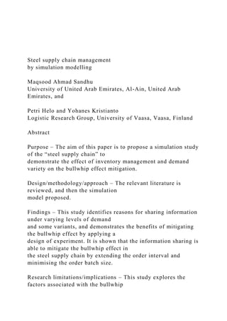
  • 31. management 55 In considering the limitation of the space, Table I exhibits an example of Stage 1 simulation results. Next, similar operations are applied to Stage 2 and 3 (Table II). 5.1 Simulation model validation and verification Table I is then analysed as performed in the ANOVA for detecting the bullwhip effect with a different level of demand and opening inventory. In the first observation, Figure 3 shows the impact of inventory level on its variance. It is clear that a high inventory level gives no advantage because a company should put a higher safety stock on this level. The reason can be retrieved from Table III. The higher level of inventory in Table III indicates that the supply chain has no precise demand information. This imprecision in the information encourages the supply chain to install a higher level of inventory. Furthermore, it affects the fill rate (delivery) variation. This combines imprecision in the demand information with that on the delivery. A similar DOE is also conducted to the supply chain with information sharing included and is benchmarked against the previous result, as shown in Table III.
  • 32. Table II shows the different performance levels between the supply chain with and without information sharing. It shows that the level of production rate and fill rate are two dependent variables affected by the demand and the beginning inventory. Input Output Run Demand Beginning inventory Final inventory Production time FC output Fill rate (product/hour) Completion rate (%) 1 75 60 23 109 73 0.69 97 2 75 60 12 147 64 0.51 85 3 75 60 33 144 72 0.52 96 4 100 60 26 246 92 0.41 92 5 100 60 31 114 93 0.88 93 6 100 60 30 282 97 0.35 97 7 125 60 23 329 125 0.38 100 8 125 60 12 294 119 0.43 95
  • 33. 9 125 60 33 286 121 0.44 97 10 75 120 79 141 74 0.53 99 11 75 120 60 159 66 0.47 88 12 75 120 72 183 72 0.41 96 13 100 120 36 226 99 0.44 99 14 100 120 53 270 99 0.37 99 15 100 120 78 272 91 0.37 91 16 125 120 79 126 125 0.99 100 17 125 120 60 85 123 1.47 98 18 125 120 72 219 121 0.57 97 19 75 180 139 123 65 0.61 87 20 75 180 128 75 71 1.00 95 21 75 180 143 117 67 0.64 89 22 100 180 116 237 99 0.42 99 23 100 180 107 276 97 0.36 97 24 100 180 97 243 100 0.41 100 25 125 180 123 309 122 0.40 98 26 125 180 75 322 123 0.39 98 27 125 180 117 231 122 0.54 98 Table I. Simulation results BIJ 20,1 56 This implies that information sharing is capable of hedging the adverse effect of the variation in the demand by adjusting the fill rate and production rate. Thus, balanced ordering rule should be appropriate to the supply chain with
  • 34. information sharing. For providing information about the level of demand magnification across the supply chain, the bullwhip effect is measured. The bullwhip effect is measured as the quotient of the demand CV generated in a given supply chain level and the demand CV received by that same level (Fransoo and Wouters, 2000), since it explicitly measures the relative variability of order against demand as an explicit representation of the bullwhip effect: Figure 3. Inventory variance as a function of beginning inventory level Inventory variance 0 100 200 300 400 500 low medium high Beginning inventory level
  • 35. V a ri a n c e Stage 1 Stage 2 Stage 3 With information sharing Without information sharing With information sharing Without information sharing With information sharing
  • 36. Without information sharing D ¼ 75 1.18 1.21 1.02 2.32 1 3.19 D ¼ 100 1.18 1.37 1.02 2.67 1 2.52 D ¼ 125 1.27 1.76 1.04 2.89 0.99 2.82 Table III. Bullwhip effect of the supply chain at different demand levels Without information sharing With information sharing Source Dependent variable F Sig. F Sig. Demand Final inventory 2.229 0.136 1.561 0.532 Fill rate 2.086 0.153 6.032 0.028 Production rate 4.777 0.022 6.773 0.023 Beginning inventory Final inventory 100.155 0 0.956 2.867 Fill rate 0.822 0.456 0.998 1.439 Production rate 0.427 0.659 1.009 1.284 Demand * beginning inventory Final inventory 2.096 0.124 1.224 0.553 Fill rate 4.859 0.008 5.194 0.072 Production rate 0.773 0.557 5.386 0.018
  • 37. Table II. Tests of between-subjects effects of Stage 1 in the supply chain with and without information sharing Steel supply chain management 57 BullwhipðBÞ ¼ sqnðtÞðt; t þ LdðnÞÞ=qnðtÞðt; t þ LdðnÞÞ sDðtÞðt; t þ LdðnÞÞ=DðtÞðt; t þ LdðnÞÞ ¼ Rout Rin : ð3Þ For sqn(t)(t,t þ Ld(n)) represents standard deviation during Ld, the lead times of delivery, qn(t)(t,t þ Ld(n)) represents the delivery rate according to the demand at time t, sD(t)(t,t þ Ld(n)) represents standard deviation demand during the delivery lead time Ld and D(t)(t,t þ Ld(n)) is the demand during the lead times.
  • 38. Table III shows that the imprecision of the demand signal is eliminated, such that variation in the delivery lead times has no significant impact on magnifying demand. The EU, as the primary funder of this research, and the research teams in Slovakia and Finland verified the model through joint efforts between the research team and the case factory. The simulation was presented before both the EU and the company representatives. After undergoing some corrective actions, finally the result was acceptable. 6. Discussion This experiment is intended to answer RQ1 about continuous replenishment and the effect of the inventory level on the order fulfilment rate (product output rate and order completion rate) and also the effect of information sharing on mitigating the bullwhip effect. Multivariate analysis of variance (MANOVA) is used in order to assess the effect of demand imprecision on the generation of the bullwhip effect. The demand and the beginning inventory level are used to indicate whether or not the information of the demand is imprecise. Thus, the final inventory level, the fill rate (delivery rate) and production rate are used as the performance indicators. Finally, demand magnification is measured through the quantification of the bullwhip effect. Tables I and II reveal the information that enhancing the quality
  • 39. of the demand information gives some advantages. First, it reduces inventory investment. Second, it informs us that the demand variation has no effect on the inventory investment, however, different order interval affects on inventory investment, with or without information sharing. The longer order interval increases the customer service level as indicated in Table I. While the longer order interval increases the service level, however it also increases the requirement about safety stocks (Figure 3). The result support Cachon (2003) conclusion where the increasing of order interval raises the supply chain cost in terms of holding and backorder costs. Furthermore, the longer order interval reduces the fill rate of the supplier as a measure of the batch size. The combination of smaller batch size and longer order interval could reduce the Bullwhip effect (Kelle and Milne, 1999; Cachon, 1999). The arrangement of the information flow has a significant effect on order completion at the agreed lead times. It is shown that allowing HRM department as supplier to access customer orders benefits the finishing department in terms of order completion rate. It implies that order amplification gives less impact to a supply chain which shares information. This result supports Dejonckeere et al. (2000, 2002) in using an APIOBPCS by providing information access to the supplier. In conclusion, this simulation gives information to readers that
  • 40. a high degree of variety of demand should not cause a bullwhip effect as long as such an order is handled individually by a continuous replenishment policy and information sharing. As a consequence, a flexible production line should be represented. BIJ 20,1 58 7. Conclusion This paper has considered information sharing in the steel supply chain. The proposed model has been successfully applied and has reduced the Bullwhip effect and has obtained related information on the production and fill rates. Moreover, the adaptive production and delivery rate are used to minimise the inventory level. This study uses a quotient of order and demand coefficient of variation, which belong, respectively, to Bullwhip measures and stock and delivery performance, in order to compare the performance of the supply chain with and without information sharing. From observing the results, it appears that the quality of demand information is improved significantly by providing a fill rate according to the demand and by reducing the inventory investment. Thus, the performances of the supply chain with information sharing seems
  • 41. to be better than its performances without information sharing (Table III). In validating the simulation model, we sent the report to the EU commission for review. The EU commission has approved the model with positive comments for the implementation of the results in the society. Further research may want to investigate a number of remaining issues. The steel supply chain must optimise the responsiveness of the production and delivery lead time to minimise the total supply chain cost. References Barber, K., Dewhurst, F., Burns, R. and Rogers, J. (2003), “Business-process modelling and simulation for manufacturing management: a practical way forward”, Business Process Management Journal, Vol. 9 No. 4, pp. 527-42. Burbidge, J.L. (1984), “Automated production control with a simulation capability”, IFIP Working Paper WG5(7), Copenhagen. Cachon, G. (1999), “Managing supply chain demand variability with scheduled ordering policies”, Management Science, Vol. 45 No. 6, pp. 843-56. Cachon, G.P. (2003), “Supply chain coordination with contracts”, in de Kok, A.G. and Graves, S.C. (Eds), Supply Chain Management: Design, Coordination and Operation, Elsevier, Amsterdam, pp. 229-340. Chang, Y. and Makatsoris, H. (2003), “Supply chain modelling
  • 42. using simulation”, International Journal of Simulation, Vol. 2 No. 1, pp. 24-30. Christopher, M. (1998), Logistics & Supply Chain Management, 2nd ed., Financial Times, London. Dale, R. (2001), “Offline programming and simulation help Boeing use giant automated riveter on C-17 aircraft”, Industrial Robot: An International Journal, Vol. 18 No. 6, pp. 478-82. Davenport, T. (1994), Process Innovation, Harvard Business Press, Boston, MA. Dawande, M., Kalagnanam, J., Lee, H.S., Reddy, C., Siegel, S. and Trumbo, M. (2004), “The slab design problem in steel industry”, INFORM, Vol. 34 No. 3, pp. 215-25. Dejonckeere, J., Disney, S.M., Lambrecht, M.R. and Towill, D.R. (2000), “Transfer function analysis of forecasting induced bullwhip in supply chains”, International Journal of Production Economics, Vol. 78, pp. 133-44. Dejonckeere, J., Disney, S.M., Lambrecht, M.R. and Towill, D.R. (2002), “Measuring and avoiding the bullwhip effect: a control theoretic approach”, European Journal of Operational Research, Vol. 147 No. 1, pp. 567-90. Djamila, O. (2003), “A multi agent system for the integrated dynamic scheduling of steel production”, PhD thesis, University of Nottingham, School of Computer Science and Information Technology, Nottingham.
  • 43. Steel supply chain management 59 Forrester, J. (1961), Industrial Dynamics, MIT Press, Cambridge, MA. Fox, M., Barbuceanu, M. and Teigen, R. (2000), “Agent oriented supply chain management”, The International Journal of Flexible Manufacturing System, Vol. 12 No. 1, pp. 165-88. Fransoo, J.C. and Wouters, M.J.F. (2000), “Measuring the bullwhip effect in the supply chain”, Supply Chain Management: An International Journal, Vol. 5 No. 2, pp. 78-89. Fu, Y.H., Piplani, R., de Souza, R. and Wu, J. (2000), “Multi- agent enabled modeling and simulation towards collaborative inventory management in supply chains”, Proceedings of the 2000 Winter Simulation Conference, Vol. 2 No. 1, pp. 1763- 71. Greasley, A. (2003), “Using business-process simulation within a business-process reengineering approach”, Business Process Management Journal, Vol. 9 No. 4, pp. 408-21. Hafeez, K., Griffiths, M., Griffiths, J. and Naim, M.M. (1996),
  • 44. “System design of two echelon steel industry supply chain”, InternationalJournalofProductionEconomics, Vol. 45 No. 1, pp. 121-30. Hammer, M. and Champy, J. (1993), Reengineering the Corporation: A Manifest for Business Revolution, HarperCollins Publisher, New York, NY. Hill, T. (1994), Manufacturing Strategy – Text and Cases, Palgrave, Basingstoke. Hlupic, V. and Vreede, G.J. (2005), “Business process modelling using discrete-event simulation: current opportunities and future challenges”, International Journal of Simulation and Process Modeling, Vol. 1 Nos 1/2, pp. 72-81. Holweg, M. and Bicheno, J. (2002), “Supply chain simulation – a tool for education, enhancement and endeavour”, International Journal of Production Economics, Vol. 78 No. 1, pp. 163-75. Hong, P., Dobrzykowski, D. and Vonderembse, M. (2010), “Integration of supply chain IT and lean practices for mass customization: benchmarking of product and service focused manufacturers”, Benchmarking: An International Journal, Vol. 17 No. 4, pp. 561-92. Jones, R.M., Naylor, B. and Towill, D.R. (2000), “Engineering the leagile supply chain”, International Journal of Agile Management Systems, Vol. 2 No. 1, pp. 54-61. Kelle, P. and Milne, A. (1999), “The effect of (s, S) ordering
  • 45. policy on the supply chain”, International Journal Production Economics, Vol. 59 Nos 1-3, pp. 113-22. Krahl, D. (2002), “The extended simulation environment”, in Yücesan, E., Chen, C.-H., Snowdon, J.L. and Charnes, J.M. (Eds), Proceedings of the 2002 Winter Simulation Conference, pp. 205-13. Law, C. and Ngai, E. (2007), “An investigation of the relationships between organizational factors, business process improvement, and ERP success”, Benchmarking: An International Journal, Vol. 14 No. 3, pp. 387-406. Lee, H.L., Padmanabhan, V. and Whang, S. (1997), “The bullwhip effect in the supply chain”, Sloan Management Review, Spring, pp. 93-102. Lee, H.S. and Murthy, S.S. (1996), “Primary production scheduling at steel-making industries”, IBM Journal of Research & Development, Vol. 40 No. 2, pp. 231-53. Levine, L. (2001), “Integrating knowledge and processes in a learning organization”, Information System Management, Vol. 18 No. 1, pp. 21-32. Lin, F. and Shaw, M.J. (1998), “Reengineering the order fulfillment process in supply chain networks”, International Journal of Flexible Manufacturing Systems, Vol. 10 No. 3, pp. 197-229. McCullen, P. and Towill, D. (2002), “Diagnosis and reduction of bullwhip in supply chains”, International Journal of Supply Chain Management, Vol. 7 No.
  • 46. 3, pp. 164-79. Metters, R. (1997), “Quantifying the bullwhip effect in supply chains”, Journal of Operations Management, Vol. 3 No. 15, pp. 89-100. Moon, S.-A. and Kim, D.-J. (2005), “Systems thinking ability for supply chain management”, Supply Chain Management: An International Journal, Vol. 10 No. 5, pp. 394-401. BIJ 20,1 60 Naylor, D.J., Bernhard, C., Green, A.M. and Sjökvist, T. (2007), Learn How to Continuously Steel on the Internet at Steeluniversity.org, available at: http://library.mcc-cdl.at/8200.pdf (accessed 12 February 2008). Paolucci, E., Bonci, F. and Russi, V. (1997), “Redesigning organisations through business process re-engineering and object-orientation”, Proceedings of the European Conference on Information Systems, Cork, Ireland, pp. 587-601. Park, H., Hong, Y. and Chang, S.Y. (2002), “An efficient scheduling algorithm for the hot coil making in the steel mini-mill”, Production Planning & Control, Vol. 13 No. 3, pp. 298-306. Rabelo, L., Sepulveda, J., Compton, J. and Turner, R. (2006),
  • 47. “Simulation of range safety for the NASA space shuttle”, Aircraft Engineering & Aerospace Technology: An International Journal, Vol. 78 No. 2, pp. 98-106. Reiner, G. and Fichtinger, J. (2009), “Demand forecasting for supply processes in consideration of pricing and market information”, International Journal of Production Economics, Vol. 118 No. 1, pp. 55-62. Sandhu, M. (2005), “Managing project business development: an inter-organizational and intra-organizational perspective”, doctoral dissertation, Swedish School of Economics and Business Administration, Helsinki. Sandhu, M. and Gunasekaran, A. (2004), “Business process development in project-based industry: a case study”, Business Process Management Journal, Vol. 10 No. 6, pp. 673-90. Swaminathan, J.R., Smith, S.F. and Sadeh, N.M. (1998), “Modeling supply chain dynamics: a multi agent approach”, Decision Sciences, Vol. 29 No. 3, pp. 607-32. Towill, D.R. (1996), “Industrial dynamics modeling of supply chains”, International Journal of Physical Distribution and Logistics, Vol. 26 No. 2, pp. 23-42. Towill, D.R. and Del Vecchio, A. (1994), “The application of filter theory to the study of supply chain dynamics”, Production Planning & Control, Vol. 5 No. 1, pp. 82-96.
  • 48. Towill, D.R., Childerhouse, P. and Disney, S.M. (2002), “Integrating the automotive supply chain: where are we now?”, International Journal of Physical Distribution & Logistics Management, Vol. 32 No. 2, pp. 79-95. Tumay, K. (1996), “Business process simulation”, Proceedings of the 28th Conference on Winter Simulation. Wilkner, J.M., Naim, M. and Rudberg, M. (2007), “Exploiting the order book for mass customized manufacturing control systems with capacity limitation”, IEEE Transactions on Engineering Management, Vol. 54 No. 1, pp. 145-55. Xiong, G. and Helo, P. (2008), “Challenges to the supply chain in the steel industry”, International Journal of Logistics Economics and Globalisation, Vol. 1 No. 2, pp. 160-75. Zhang, H., Li, H. and Tam, C. (2004), “Fuzzy discrete-event simulation for modeling uncertain activity duration”, Engineering, Construction and Architectural Management, Vol. 11 No. 6, pp. 426-37. Further reading Hammer, M. (2007), “The process audit”, Harvard Business Review, April. Corresponding author Maqsood Ahmad Sandhu can be contacted at: [email protected] To purchase reprints of this article please e-mail: [email protected] Or visit our web site for further details:
  • 49. www.emeraldinsight.com/reprints Steel supply chain management 61 Reproduced with permission of the copyright owner. Further reproduction prohibited without permission. IBM SPSS Step-by-Step Guide: t Tests Note: This guide is an example of creating t test output in SPSS with the grades.sav file. The variables shown in this guide do not correspond with the actual variables assigned in Unit 8 Assignment 1. Carefully follow the Unit 8 Assignment 1 instructions for a list of assigned variables. Screen shots were created with SPSS 21.0. Assumptions of t Tests To complete Section 2 of the DAA for Unit 8 Assignment 1, you will generate SPSS output for a histogram, descriptive statistics, and the Shapiro-Wilk test. (Levene test output will appear in Section 4 of the DAA). Refer to the Unit 8 assignment instructions for a list of assigned variables. The examplevariables lowup and final are shown below. Step 1. Open grades.sav in SPSS. Step 2. Generate SPSS output for the Shapiro-Wilk test of normality. (Refer to previous step-by-step guides for generating
  • 50. histogram output and descriptives output for the Unit 8 assignment variables.) · On the Analyze menu, point to Descriptive Statistics and click Explore… · In the Explore dialog box, move the assigned Unit 8 variables into the Dependent List box. The final variable is used as an example below. · Click the Plots… button. · In the Explore: Plots dialog box, select the Normality plots with tests option. · Click Continue and then OK. Step 3. Copy the Tests of Normality table and paste it into Section 2 of the DAA Template. Interpret the output. Note: The Levene test is also generated as part of the SPSS t- test output for Section 4 (discussed next). You do not have to provide the Levene test output twice. You can report and interpret it in Section 2 and then provide the actual output in Section 4. Reporting of t Tests DAA Section 4 involves generating the t-test output and interpreting it. The example variables of lowup (lower division = 1; upper division = 2) and final are shown below. Step 1. Generate SPSS output for the t test. · On the Analyze menu, point to Compare Means and click Independent-Samples T Test…
  • 51. Step 2. In the Independent-Samples T Test dialog box: · First, move the Unit 8 Assignment 1 dependent variable into the Test Variable(s) box. · Second, move the Unit 8 assignment variable into the Grouping Variable box. Notice the (? ?) after the variable. The values of the independent variable are assigned in the next step. · Third, click the Define Groups… button. · Fourth, in the Define Groups dialog box, assign the corresponding values: Group 1 = 1, Group 2 = 2. · Fifth, click Continue and then OK. Step 3. Copy the output for the independent samples test and paste it into Section 4 of the DAA Template. Then interpret it as described in the Unit 8 assignment instructions. 2 Running head: DATA ANALYSIS AND APPLICATION TEMPLATE 1 DATA ANALYSIS AND APPLICATION TEMPLATE 2Data Analysis and Application (DAA) Template Name University Data Analysis and Application (DAA) Template
  • 52. Use this file for all assignments that require the DAA Template. Although the statistical tests will change from week to week, the basic organization and structure of the DAA remains the same. Update the title of the template. Remove this text and provide a brief introduction.Section 1: Data File Description 1. Describe the context of the data set. You may cite your previous description if the same data set is used from a previous assignment. 2. Specify the variables used in this DAA and the scale of measurement of each variable. 3. Specify sample size (N). Section 2: Testing Assumptions 4. Articulate the assumptions of the statistical test. 5. Paste SPSS output that tests those assumptions and interpret them. Properly integrate SPSS output where appropriate. Do not string all output together at the beginning of the section. 6. Summarize whether or not the assumptions are met. If assumptions are not met, discuss how to ameliorate violations of the assumptions.Section 3: Research Question, Hypotheses, and Alpha Level 1. Articulate a research question relevant to the statistical test. 2. Articulate the null hypothesis and alternative hypothesis. 3. Specify the alpha level.Section 4: Interpretation 1. Paste SPSS output for an inferential statistic. Properly integrate SPSS output where appropriate. Do not string all output together at the beginning of the section. 2. Report the test statistics. 3. Interpret statistical results against the null hypothesis.Section 5: Conclusion
  • 53. 1. State your conclusions. 2. Analyze strengths and limitations of the statistical test.References Provide references. International Journal of Production Research Vol. 50, No. 16, 15 August 2012, 4699–4717 Impact of the pull and push-pull policies on the performance of a three-stage supply chain Santosh Mahapatra*, Dennis Z. Yu and Farzad Mahmoodi School of Business, Clarkson University, 311, Bertrand H. Snell Hall, Potsdam, NY 13699, USA (Received 4 January 2011; final version received 23 October 2011) We investigate the performance of two common operating policies (i.e., pull and push-pull) for a make- to-stock product in an un-capacitated, three-stage supply chain. The pull policy operates based on periodic orders received from the immediate downstream facility. However, in the push-pull policy, while processes upstream of the order decoupling point are managed by the push policy, the downstream processes are managed by the pull policy. Simulation experiments are conducted to examine the impact of each operating policy under a variety of experimental conditions, characterised by demand uncertainty and lead-time variability. Our results indicate that the relative advantage of
  • 54. the two policies is dependent on the type of uncertainty, the level of uncertainty, the inventory control policy and the performance measures of interest. More specifically, while the push-pull policy results in lower inventory, the pull policy yields a better fill rate. This is in contrast to the notion that the pull policy generally results in superior inventory performance. Our findings suggest that firms should carefully consider the level of uncertainty, the inventory control policy and the performance measures of interest when determining the operating policy. Keywords: pull policy; push-pull policy; demand uncertainty; lead-time variability; operational performance; simulation research 1. Introduction It is challenging to manage a multi-stage supply chain in an environment characterised by uncertain customer demand and variable manufacturing and distribution lead-times. In such environments, the performance of a multi- stage supply chain is manifested in terms of excess inventory, poor customer service, or both. The push, pull and push-pull (referred to as ‘hybrid’ here thereof) operating policies are the three principal policies utilised to control production and distribution systems (Karmarkar 1990). Whilst in the push policy sourcing and production and distribution processes are purely based on anticipated demand, or forecast, in the pull policy such processes are triggered after the customer order is received (Spearman and Zazanis 1990). Alternatively, in the hybrid policy, processes upstream of the order decoupling point (i.e. point of differentiation) are managed by the push policy, while the processes downstream of the order decoupling point are managed by the pull policy (Pyke and
  • 55. Cohen 1990). While several studies have examined the push, pull or hybrid policies in a single-stage supply chain, evaluation of the policies in a multi-stage supply chain is rather limited and the insights are either incomplete or case-specific (see Masuchun et al. 2004). This can be attributed to a higher level of operational challenges in multi-stage supply chains than in single-stage chains. As such a comparative assessment of the three policies is difficult because the workings of the three policies are distinctly different, and the criteria for evaluating the performance while accounting for the difference in their workings are not clearly outlined. To address the knowledge gap, we investigate the performance of two of the three policies (i.e. pull and hybrid policies), while accounting for the basic tenets of the push and pull-based operations. Our study involves a storable product in a three-stage supply chain consisting of a manufacturing plant, a warehouse and retailer(s). We do not analyse the case when the push policy is implemented throughout the supply chain. Such practice is fairly unrealistic since in a typical multi-stage supply chain at least one of the upstream facilities initiates production based on orders from the downstream facilities. The operating policies are carried out independently at the three facilities meaning the information (e.g. forecasts or orders) that triggers actions is generated locally. The decentralised characterisation of the operations is consistent with the ‘push’ or ‘pull’ fundamentals (e.g. Pyke and Cohen 1990, Spearman and *Corresponding author. Email: [email protected] ISSN 0020–7543 print/ISSN 1366–588X online � 2012 Taylor & Francis
  • 56. http://dx.doi.org/10.1080/00207543.2011.637091 http://www.tandfonline.com Zazanis 1990) and reflects the typical scenario of limited access to information regarding other firms in a multi-stage supply chain. It is often conjectured by both practitioners and researchers that performance of the pull policy is generally superior to the push policy (Spearman and Zazanis 1990). Although the hybrid policy combines the push and pull policies, the conjecture regarding superior performance of the pull policy does not hold as strongly when compared with the hybrid policy. Previous studies have shown that the performance of the pull and hybrid policies is affected by demand uncertainty, forecast error and buffer stock levels (e.g. Masuchun et al. 2004). However, these studies have not systematically examined how lead-time uncertainty and buffer stocks affect performance across the two policies. In the extant studies, the inventory policies, specifically the buffer stocks, have been chosen somewhat arbitrarily. Consequently, the relative efficacy of the two policies remains unclear. We address these issues by examining the performance dynamics under varied levels of demand uncertainty and production/distribution lead-time variability when the buffer stocks are chosen for a specified service level. Specifically, our study intends to answer the following research questions: (1) How do demand and lead-time uncertainties affect the performance of a three-stage supply chain?
  • 57. (2) How do the performances of the pull and hybrid policies differ in a three-stage supply chain? We utilise simulation models in our analysis because the simultaneous impact of multiple types of uncertainties such as demand uncertainty, lead-time uncertainty and forecast error is very difficult to examine analytically in a multi-stage supply chain. The remainder of the paper is organised as following. The relevant literature is reviewed in the next section. This is followed by a description of the supply chain structures considered, simulation models and assumptions, as well as the experimental design. Then, the simulation results for a single retailer supply chain are discussed. This is followed by a sensitivity analysis for a multiple retailer supply chain. Finally, the conclusions and managerial implications of the study are presented. 2. Literature review Several studies have examined the effectiveness of the push, pull and hybrid policies under a variety of operating conditions; however, they differ significantly in the implementation of the three policies. Since the push and pull policies are fundamental to characterise the alternate policies, it is useful to understand their distinctions. Pyke and Cohen (1990) characterised the differences between the push and pull policies in terms of production and order quantity, timing of the production and shipment request, order prioritisation rules and degree of managerial interference. On the other hand, Bonney et al. (1999) characterised the push and pull policies in terms of the flow of control information. In a pull system the control information flow typically is in the opposite direction of the material flow. In contrast, the control information flow in a
  • 58. push system is in the same direction as the material flow. Furthermore, while in the pull system a downstream facility with primarily local information exercises a greater decision authority regarding the volume of supplies to receive from the upstream facility, in the push system the upstream facility with information that may be local or global has a greater decision authority regarding the volume of dispatch to the downstream facility (Pyke and Cohen 1990). Spearman and Zazanis (1990) noted that the operating principles of the push and pull policies are radically different. They observed that the push policy controls operations in terms of production or distribution plan and measures performance through work-in-progress (WIP) inventory. In contrast, the pull policy controls operations in terms of the level of WIP inventory and measures performance in terms of the unmet demand. Extant researchers have utilised analytical and simulation based approaches to evaluate the performance of the three alternate operating policies. While the analytical studies (e.g. Spearman and Zazanis 1992, Pandey and Khokhajaikiat 1996, Vidyarthi et al. 2009) utilised inventory and queuing models to establish a functional relationship between the various control variables in relatively simple operating contexts, simulation studies (e.g. Bonney et al. 1999, Maschun 1999, Li 2003, Maschun et al. 2004) explored the interactions among a large number of variables in relatively more complex operating contexts. Most of the analytical studies have dealt with either deterministic scenarios (e.g. Wang and Sarker 2006) or stochastic analysis in relatively simple settings (e.g. Spearman and Zazanis 1992, Pandey and Khokhajaikiat 1996). Vidyarthi et al. (2009) utilised queuing theory to develop analytical models to minimise response time while
  • 59. optimally allocating workloads and creating capacity in make- to-order and assemble-to-order supply chains. 4700 S. Mahapatra et al. Their study did not analyse the performance of the push policy for firm orders. Consequently, it provided limited insights into the relative performance of the three policies. Wang and Sarker (2006) proposed non-linear mixed integer programming models for optimal Kanban-based control of a manufacturer, warehouse and retailer supply chain with deterministic demand and lead-time. The study illustrated the usefulness of Kanban-based pull policy but did not offer insights into its relative advantages over alternative operating policies. Pandey and Khokhajaikiat (1996) examined the performance of the three alternate policies in a production system that was modelled as a discrete time Markov process. The system accounted for supply and production lead- time uncertainty, demand uncertainty and raw material constraints. They noted that no policy is distinctly superior at all levels of demand uncertainty. While the performance of the hybrid policy was generally superior, the push policy (i.e. MRP based lot sizing) outperformed the hybrid policy in the presence of raw material constraints. The performance of the pull policy (i.e. Kanban based) was superior only when the demand was very stable. Spearman and Zazanis (1992) compared the performance of the push and pull systems when processing time follows a Poisson distribution, while demand is exponentially distributed. They observed that the pull policy is easier to control and performs better than the push policy because in the pull policy the WIP inventory is bounded; however, the hybrid
  • 60. policy (i.e. pull policy only at the final stage) can outperform pure push and pull policies. A few studies attempted to combine analytical approaches with simulation approaches (e.g. Gonçalves et al. 2005, Su et al. 2010). In general, these studies formulated models to describe the operations. The effectiveness of these models was subsequently assessed using simulation. For example, Gonçalves et al. (2005) formulated a model for analysing the effect of demand uncertainty in a hybrid system. Su et al. (2010) developed an M/M/1 base-stock model to evaluate the effectiveness of delayed differentiation when there are arrival and production variability in a single-stage push system. Both studies utilised simulation to obtain the performance results. It is apparent that it is difficult to develop analytical models to compare the performance of the three policies while capturing the underlying details. Consequently, past studies (e.g. Spearman and Zazanis 1992) have recommended simulation studies to determine the effectiveness of alternate policies. In a recent study, Almeder et al. (2009) observed that analytical and simulation based researches should serve as complements in studying supply chains. In a typical supply chain, activities such as manufacturing, warehousing and distribution have dissimilar task complexities and lead-times, and are spatially and temporally dispersed. These elements in combination affect the supply chain performance; the combined impact of these factors in a multi-stage supply chain has not been examined adequately. In particular, most of the previous studies (e.g. Closs et al. 1998, Grosfeld-Nir et al. 2000, Kim et al. 2002, Li 2003, Masuchun et al. 2004, Teeravaraprug and Stapholdecha 2004) do not examine how the supply chain performance is affected by different levels of demand uncertainty and lead-time variability.
  • 61. The implementation and performance of the push, pull and hybrid policies vary significantly from study to study. In general, the studies differ in terms of the assumptions regarding the inventory control policy, demand uncertainty, lead-time variability, location of the order decoupling point and knowledge of demand information which affect the performance. Furthermore, most of the studies do not explicitly account for forecast error, a key determinant of the efficacy of push-based operations. Forecast errors, usually include two components (i.e. variability and bias), which have a significant impact on the firm’s operational performance (Lee and Everett 1986, Ritzman and King 1993). Forecast error is influenced by the operational planning horizon, which is dependent upon the operational lead-times and the frequency of plan updates. The longer the planning horizon, the higher is the forecast error (Chen et al., 2000). Based on a study of population forecast errors, Smith and Sincich (1991) concluded that there exists a linear or nearly linear relationship between forecast inaccuracy and the length of the forecast horizon. Therefore, it is useful to include these considerations while accounting for the forecast errors. As noted earlier, the existing studies are somewhat arbitrary in their choice of the inventory policy. For example, while some papers keep the same level of safety stocks for the various policies to maintain comparability (e.g. Pandey and Khokhajaikiat 1996, Closs et al. 1998), others adjust the safety stocks arbitrarily with the change in demand (e.g. Bonney et al. 1999, Masuchun et al. 2004). Most of the studies have reported the snapshot performance of the various operating policies (e.g. Closs et al. 1998), ignoring to reveal how the performance changes over time. Prior studies have used a variety of performance measures such as fill rate, throughput rate,
  • 62. system inventory, retailer inventory, production lead-time, inventory costs and the variability of fill rate. These measures can be broadly classified into three categories: order fulfilment rate, cycle time and inventory level. Reporting of results in multiple forms presents difficulty in comparing the performance. To address some of the above shortcomings this study considers the impact of forecast error, demand uncertainty and lead-time variability on the inventory and fill rate performance of the pull and hybrid policies. We examine both longitudinal and snapshot results for the two performance metrics. The experimental environment International Journal of Production Research 4701 including the supply chain structures, simulation models, assumptions as well as the experimental design are discussed next. 3. Experimental environment Our study considers a single-product supply chain with geographically dispersed facilities. The supply chain consists of a manufacturing plant, a warehouse and a retailer (or three retailers in the multiple retailer system), and is affected by varied levels of demand uncertainty and lead-time variability. It is assumed that there is no capacity constraint at any of the facilities. Labeling, packaging and shipping operations are conducted in the warehouse. The warehouse acts as a stocking point and supplies the retailer(s) according to orders received from them. In the hybrid policy, the warehouse receives supplies from the plant according to demand forecasts at the plant; however, in the
  • 63. pull policy, the warehouse receives supplies according to the orders placed to the plant. Thus, the warehouse acts as the order decoupling point in the hybrid policy. By assigning the warehouse as the order decoupling point, we are able to implement the pull operating policy to all or a part of the supply chain. Two types of inventories (i.e. inputs and outputs) are held at the plant and the warehouse. However, only one type of inventory (finished goods) is held at the retailer. The supply chain structures considered in the study are depicted in Figure 1(a) and 1(b). There are multiple lead-times in the supply chain: LT1 is associated with the outside supplier (i.e. it takes LT1 days for the plant to receive a raw material order from the supplier); LT2 is the production lead-time; LT3 is the transportation lead-time between the plant and the warehouse; LT4 is the warehouse assembling lead-time; and LT5 is the distribution lead-time between the warehouse and the retailer(s). Implementation of the push and pull policies can be carried out in multiple ways (Pyke and Cohen 1990, Hopp and Spearman 2004). In our model, the operations in the pull policy at all upstream facilities are carried out based on the replenishment orders from the immediate downstream facility. The facilities review the inventory level (local stock plus pipeline inventory) at the beginning of each week and place an order to bring the inventory to the order- up-to-level which is determined by the average demand during the protection interval (the sum of the time period between two successive reviews and the supply lead-time), plus safety stocks to avoid shortage during the protection interval. However, in the hybrid policy, while the operations at the plant and dispatch to warehouse are governed by the forecast requirements as in the push policy, the operations and order fulfilments at the warehouse and the
  • 64. retailer(s) are governed by actual orders as in the pull policy. Thus, the plant develops the production plan based on the customer demand forecasts and safety stock requirements, without the knowledge of downstream inventory levels. In the hybrid policy, the safety stocks for the push based operations are maintained to avoid shortage during the supply lead-times. Pure forecast-based fulfilment from the plant to the warehouse represents poor information flow between the warehouse and the plant (Pyke and Cohen 1990). Note that such unco-ordinated supply chains characterised by the lack of cross-company integration and poor information flow are observed in a variety of industries (Davis and Spekman 2004). Figures 2 and 3 illustrate the operational details of the pull and hybrid policies, respectively. Plant (b) (a) Warehouse Supplier Purchasing Production Assembly Distribution LT1 LT4 LT3 LT2 LT5 Customer
  • 65. Retailer Plant Warehouse Supplier Purchasing Production Assembly Distribution LT4 LT3 LT2 LT1 LT5 Customer Customer Customer Retailer 1 Retailer 2 Retailer 3 Figure 1. (a) Supply chain structure: single retailer system; (b) Supply chain structure: multiple retailer system. 4702 S. Mahapatra et al. We assume that the supplier has enough capacity to fulfil all
  • 66. orders from the plant. Nevertheless, raw material safety stocks are held at the plant to cover for the demand and supplier-to-plant transportation lead-time uncertainties. The supplies from the plant and warehouse are constrained by the available inventory. The unmet demands at the plant and the warehouse are backlogged and manufactured with a lag in the pull policy. However, in the hybrid policy only the shortages of inputs that lead to production shortfalls at the plant are backlogged (refer to Figure 2). The input shortages at the warehouse and output shortages at the plant are not backlogged because the respective supplies occur based on push principles. Accordingly, replenishment order for the input at the plant is based on the forecast demand for week (t), the input safety stock and the input shortage. At the retailer, if there is insufficient inventory to satisfy the customer demand, the unmet demand is lost without backordering in both policies. The supply chain structure allows postponement strategy in packaging and shipping (i.e. operations that move labelling processes such as language required, product stickers and user manuals to the final phase of packaging). Postponement processes produce generic products, which are later customised upon receipt of an order. For example, Hewlett-Packard has applied this strategy to packaging and labelling of printers before shipping to customers (www.kongandallan.com, 10 June 2007). Other examples of the postponement strategy in packaging and shipping include fast moving consumer goods companies that sell a product under various brand names or in
  • 67. various packaging sizes. The principles for the push and pull policies in our study are illustrated below in terms of production at the plant and dispatch quantities to the warehouse. Customer’s/retailer’s/warehouse’s order arrives Retailer/warehouse/plant checks if available inventory can satisfy the order? Satisfy customer’s /retailer’s / warehouse’s order and update retailer’s/warehouse’s /plant’s inventory status Backlog any shortage at warehouse /plant and send available inventory to retailer/warehouse No Yes Calculating order -up-to level at retailer/warehouse /plant according to anticipated customer demand during the protection interval
  • 68. Retailer /warehouse /plant checks if available inventory is less than the order-up-to level? Retailer/warehouse /plant orders the difference between inventory and order -up-to level No action is needed No Yes Figure 2. Illustration of the pull policy. International Journal of Production Research 4703 Push policy: Production at the plant and dispatch quantities to the warehouse: Forecast requirement for week (t) from plant¼forecast demand for week (t)þsafety stock at the warehouse where, safty stock ¼ ffiffiffiffiffiffiffiffiffiffiffiffiffiffiffiffiffiffiffiffiffiffiffiffiffiffi ffiffiffiffiffiffiffiffiffiffiffiffiffiffiffiffiffiffiffiffiffiffiffiffiffiffi ffiffiffiffiffiffiffiffiffiffiffiffiffiffiffiffiffiffiffiffiffiffiffiffiffiffi ffiffiffiffiffiffiffiffiffiffiffiffiffiffiffiffiffiffiffiffiffiffiffiffiffiffi ffiffiffiffiffiffiffiffiffiffiffiffiffiffiffiffiffiffiffiffiffiffiffiffiffiffi ffiffiffiffiffiffiffiffiffiffiffiffiffiffiffiffiffiffiffiffiffiffiffiffiffiffi
  • 69. ffiffiffiffiffiffiffiffiffiffiffiffiffiffiffiffiffiffiffiffiffiffiffiffiffiffi ffiffiffiffiffiffiffiffi ½vaciance of weekly demand in week ðtÞ �avg: manuf: and warehouse delivery lead-time in weeks�þ ½squared avg: weekly demand in week ðtÞ �variance of manuf: and warehouse delivery lead-time in week� z vuuuuut and z standardised normal distribution statistic for the specified service level Production is carried out if and only if: Output inventory at the plant in week (t)5 forecast requirement for week (t) Production at the plant for week (t)¼min [forecast requirement for week (t), potential output by the available input inventory in week (t)] Shortages of inputs at plant in week (t)¼max [required inputs for producing the forecast requirement for week (t) – available input inventory in week (t), 0] Dispatch to the warehouse for week (t)¼min [forecast requirement for week (t), output inventory at the plant in week (t)]
  • 70. Pull policy: order to the plant and dispatch to the warehouse Warehouse’s (input) order-up-to-level while reviewing for week (t) ¼average demand during the protection intervalþsafety stock at the warehouse where, safety stock ¼ ffiffiffiffiffiffiffiffiffiffiffiffiffiffiffiffiffiffiffiffiffiffiffiffiffiffi ffiffiffiffiffiffiffiffiffiffiffiffiffiffiffiffiffiffiffiffiffiffiffiffiffiffi ffiffiffiffiffiffiffiffiffiffiffiffiffiffiffiffiffiffiffiffiffiffiffiffiffiffi ffiffiffiffiffiffiffiffiffiffiffiffiffiffiffiffiffiffiffiffiffiffiffiffiffiffi ffiffiffiffiffiffiffiffiffiffiffiffiffiffiffiffiffiffiffiffiffiffiffiffiffiffi ffiffiffiffiffiffiffiffiffiffiffiffiffiffiffiffiffiffiffiffiffiffiffiffiffiffi ffiffiffiffiffiffiffiffiffiffiffiffiffiffiffiffiffiffiffiffiffiffiffiffiffiffi ffiffiffiffiffiffiffiffiffiffi variance of weekly demand in week ðtÞ � avg. manuf. and warehouse delivery lead-time in weeksþ review period in weeks � �� � þ½squared avg. weekly demand in week ðtÞ �variance of manuf. and warehouse delivery lead-time in weeks] z vuuuuuut
  • 71. Customer demand forecasts at plant for week t Enough output inventory at plant? Calculation of required output at plant Calculation of required input at plant accounting for shortage No Yes Dispatch available output to warehouse and produce required output at plant and update inventory status Sourcing raw material if necessary Dispatch required output to warehouse and update inventory status Customer’s/retailer’s order arrives
  • 72. Retailer/warehouse checks if available inventory can satisfy the order? Satisfy customer’s/retailer’s order and update retailer’s/ warehouse’s inventory status Backlog any shortage at warehouse and send available inventory to retailer No Yes Calculating order-up-to level at retailer/warehouse according to anticipated customer demand during the protection interval Retailer/warehouse checks if available inventory is less than the order-up-to level? Retailer orders/warehouse assembles the difference between inventory and order-up-to level No action is needed
  • 73. No Yes Figure 3. Illustration of the hybrid policy. 4704 S. Mahapatra et al. Replenishment order is placed to the plant if and only if: (input) inventory at the warehouse in week (t) 5 order-up-to- level for week (t) Order quantity to the plant for week (t)¼max [order-up-to-level for week (t) – (input) inventory at the warehouse in week (t)þshortages of inputs in week (t), 0] Where, shortages of inputs in week (t)¼min [0, (input) inventory at the warehouse in week (t) – warehouse output’s order quantity for week (t)] Input inventory at the warehouse includes the inventory in transit between the plant and the warehouse. Dispatch to the warehouse for week (t)¼min [warehouse’s order to the plant for week (t), available inventory at the plant in week (t)] Next, we describe the functional forms for demand and forecast that are used to generate safety stocks, and production and dispatch requirements. We adopt the following demand function from Zhao et al. (2002) to generate
  • 74. the customer demand at the retailer. The weekly demand function is given by the following equation: Demandt ¼ baseþ slope� tþ season� sin 2� SeasonCycle � t � � þnoise� snormal ðÞ ð1Þ where, Demandt is defined as the demand in week t, snormal() represents the standard normal distributed random number generator, and SeasonCycle represents the weekly demand effects (set to four in this study). The parameters base, slope, season and noise characterise the level, growth, seasonality and variability of the demand process, respectively. The noise is expressed as a percentage of the base demand. During the simulation, the average demand for a specific week t is given by the first three terms of the demand function. The standard deviation of demand for computing safety stocks is calculated by the product of the average demand and the coefficient of variation which is generated according to the demand samples of Equation (1). We utilise the above demand function because it is comprehensive and includes the key elements that typically characterise the demand in practice.
  • 75. In the push policy, the demand forecast for week t, Forecast , made in week t0 for (t�t0) is generated by the following equation (Zhao et al. 2002): Forecastt ¼ Demandt �f1þEBþED�½1þðt� t0Þ=4:85�� snormal ð Þg ð2Þ Forecasti has two components: customer demand during week (t) and a forecast error coefficient which consists of three components. The three components of forecast error term are: the bias (EB), the variability (ED) which is normally distributed, and a parameter (i.e. 1/4.85) representing the rate of linear increase in ED with time to account for higher forecast error for higher forecast horizon (e.g. t � t0). The forecast accuracy, forecast horizon, expected lead-times and targeted service level are maintained as control variables. The forecast horizons for procurement and production at the plant are 7 and 6 weeks, respectively. Note that the forecast horizon at the plant is longer than the average supplier procurement and production lead-time. This is consistent with the practice at many firms that utilise a longer forecast horizon than the actual transportation and manufacturing lead-time to account for developing the forecast, communicating with the supplier or internal divisions, arranging for resources, etc. that are extraneous to the operations considered in our analysis.
  • 76. We examine the performance implications through a series of experiments. In our experiments, we consider three levels of lead-time variability (i.e. LT standard deviation), as well as three levels of demand uncertainty (i.e. noise). The lead-time variability is assumed to be normally distributed (Bowersox et al. 2002). We vary the manufacturing lead-time variability at the plant, the transit lead-time variability between the plant and the warehouse and the transit lead-time variability between the warehouse and the retailer. However, we do not vary the variability of supplier lead-time because in a typical supply chain, contracts are often executed to ensure timely supplier delivery and the manufacturer can hold the supplier responsible for poor delivery performance. We also do not vary the variability of warehouse processing lead-time as the activities in a warehouse are comparatively simpler and unlikely to vary significantly. In summary, we consider different levels of lead-time variability that are more relevant to the manufacturer as well as those that involve comparatively complex processes and more likely to vary. Across all experiments, the safety stocks are maintained for a specified customer service level in both policies and the forecast error in the hybrid policy is considered fixed. Thus, the experimental variables used in the study are:
  • 77. . Two operating policies: pull and hybrid International Journal of Production Research 4705 . Production, transportation and distribution lead-time variability levels (LT Std dev): for LT2, LT3 and LT5, with an average of 3 days and standard deviation of 0.5, 1 and 1.5 days, respectively . Three demand uncertainty levels (noise): (10%, 20%, 30%)�base. Accordingly, a 2�3�3 full factorial experiment with 30 replications is conducted, resulting in 540 models. The main assumptions considered in our models can be summarised as: (1) The entities operate in a decentralised manner. Each facility takes decisions based on locally available inventory and shortage information. (2) The operations at the plant, the warehouse and the retailer(s) are not affected by capacity constraints. (3) Lead-time uncertainty, demand uncertainty and forecast error are normally distributed. (4) Noise and lead-time parameters remain constant over time and are independent of each other. The parameters used in the simulation models are summarised in Table 1. The numerical values for the parameters are hypothetical. However, the values are comparable to those in fast moving consumer goods industry
  • 78. and were set based on discussions with the executives who participated in the Global Supply Chain Management Executive Seminar held at Clarkson University, USA, in August 2009. In a given context appropriate data may be chosen to derive useful insights. ARENA V12.0 was utilised to develop the simulation models (Kelton and Sadowski 2004). This software is widely used in simulation studies (e.g. Closs et al. 1998, Masuchun et al. 2004, Teeravaraprug and Stapholdecha 2004). The models were started in an empty and idle state and the first 26 weeks of data were truncated to account for the warm- up period. Note that input inventory accumulates at the warehouse due to the mismatch between the forecast based supply from the plant and the downstream demand in the hybrid policy. Consequently, the steady-state condition will not be reached for the input warehouse inventory in the corresponding simulation models. Therefore, we utilise a terminating simulation in our analysis. In practice, firms utilising the push or hybrid policies engage in flushing inventory in a variety of ways (e.g. halting production) from time to time (Spearman and Zazanis 1992, Hopp and Spearman 2004). We do not allow flushing out accumulated inventory in our models to avoid the inclusion of confounding variables while trying to compare the performance
  • 79. of the two policies. In our analysis, we use the overall system inventory, the inventory level at the retailer(s), and fill rates at the retailer(s) as performance metrics. Fill rate and inventory levels are common performance indicators used in the previous studies (e.g. Closs et al. 1998). Statistics were collected for 78 weeks after the warm-up period. It was determined via pilot runs that 20 replications would achieve the sufficient precision needed to estimate the mean differences in performance (Kelton et al. 2004). Yet, 30 replications were completed to allow the assumption of the law of large number to apply so that normality conditions can be invoked in the data analysis. Table 1. Summary of simulation model parameters. Features Parameters Demand model Base¼100 units (300 for multiple retailer system) Slope¼5/52 Season¼1 SeasonCycle¼4 Noise¼10%, 20%, 30% (experimental variable) Snormal(): standard normal distribution Forecasting model Mean of forecast errors: EB¼0 Initial variability: ED¼5% Increase rate: 1/4.85
  • 80. Snormal(): standard normal distribution Lead-time (days) LT1: mean¼5, standard deviation¼1 LT2: mean¼3, standard deviation¼0.5, 1, 1.5 (experimental variable) LT3: mean¼3, standard deviation¼0.5, 1, 1.5 (experimental variable) LT4: mean¼1, standard deviation¼0.5 LT5: mean¼3, standard deviation¼0.5, 1, 1.5 (experimental variable) Service level Desired service level: 98% 4706 S. Mahapatra et al. 4. Discussion of simulation results The performance of the two operating policies is measured on a weekly basis in terms of item fill rate at the retailer, inventory level at the retailer, the inventory upstream of the warehouse (i.e. the inventory at the plant, plus the input inventory at the warehouse), and the system inventory (i.e. the total inventory at the plant, the warehouse and the retailer). In a three-stage supply chain, inventory level and fill rate at any stage are influenced by both the inventory policy and the supply-demand dynamics. Prior studies have primarily reported snapshot results that do not reflect the performance dynamics adequately (e.g. Closs et al. 1998, Kim et al. 2002). We report both longitudinal and snapshot results to address the issue. Longitudinal analysis involves weekly average performance across the 30 replications over time to capture the supply-demand dynamics. Snapshot analysis involves
  • 81. comparisons of performance of the 30 replications at three distinct times: week 52, week 78 and week 104. To make a statistical assessment of the extent of association between the experimental and performance variables we pooled the data across the two operating policies and conducted regression analysis while using the experimental variables, the demand, the time period as the independent variables, and each of the performance variables as the dependent variables. In the longitudinal analyses, time series data were adjusted for auto-correlation when auto-correlation was noted (i.e. Durbin-Watson statistic was outside the 1.5–2.5 range suggested by Hansen and Fisher (1980)). In the regression analysis, the operating policies and snapshot time points are represented as dummy variables. Note that the base case represents the pull policy. In addition, in snapshot analysis, week 52 represents the base case. The results are presented in Tables 2–5 and Figures 4–14. In the figures we limit our presentations to the highest and lowest levels of demand uncertainty and lead-time variability. We compare and contrast our analysis of the performance impact of the pull and hybrid operating policies with those of the past studies. We first present the results for the single retailer supply chain, and subsequently discuss how the results differ for the multiple retailer case. 4.1 Average retailer inventory (longitudinal analysis) It is apparent from the regression results (see Table 2) that the average retailer inventory level is marginally lower in the hybrid policy. The results further indicate that the inventory levels increase with demand uncertainty (Noise), the lead-time variability (LT standard deviation) and the demand; however, there is no significant increase in inventory over time (Week). Among the three significant influencing
  • 82. variables, demand is noted to be the most influencing variable. Interestingly, we find that the effects of lead-time variability and demand uncertainty are practically small. Given that the inventory increase reflects the combined effects of demand, degree of uncertainty (i.e. safety stock) and supply-demand mismatch, our results indicate that the change in the level of inventory over time is mostly driven by the change in the level of demand. These results are fairly similar to the finding of Closs et al. (1998) that the retailer inventory level is somewhat insensitive to demand uncertainty. Note that our experimental environment Table 2. Regression results for the single retailer case. The regression coefficients refer to standardised coefficients. Longitudinal data analysis. Average retailer inventory* Average inventory upstream of the warehouse* Average system inventory* Average retailer fill rate Adjusted R 2 0.928 0.258 0.730 0.775 F statistic (df¼1367) 3530.920 96.120 741.820 787.673
  • 83. Intercept (un-standardised) �12.212 �14.247 13.256 0.739 Hybrid �0.025 0.302 �0.141 0.042 Week 0.005 ns 0.102 0.035 �0.148 Noise 0.067 0.127 0.083 �0.552 LT standard deviation 0.064 0.239 0.028 �0.203 Demand 0.955 0.224 0.783 �0.017 ns Retailer inventory NA NA NA 1.315 Notes: *Adjusted for auto-correlation; ns, non-significant; significance level, p5 0.05. International Journal of Production Research 4707 Table 4. Regression results for the multiple retailer case. The regression coefficients refer to standardised coefficients. Longitudinal data analysis. Average retailer inventory* Average inventory upstream of the warehouse*
  • 84. Average system inventory* Average retailer fill rate Adjusted R 2 0.516 0.935 0.904 0.770 F statistic (df¼1367) 292.118 3924.645 2582.171 761.650 Intercept (un-standardised) 3.857 �37.124 �6.482 0.725 Hybrid 0.021 �0.075 �0.107 0.037 Week 0.024 0.022 0.023 �0.157 Noise �0.099 0.064 0.052 �0.541 LT standard deviation 0.126 0.049 0.055 �0.196 Demand 0.645 0.912 0.880 �0.003 ns Retailer inventory NA NA NA 1.299 Notes: *Adjusted for auto-correlation; ns, non-significant; significance level, p 5 0.05. Table 5. Regression results for the multiple retailer case. The regression coefficients refer to standardised coefficients. Snapshot data analysis. Retailer inventory
  • 85. Upstream inventory at the warehouse System inventory Service level Adjusted R 2 0.583 0.391 0.488 0.114 F statistic (df¼1619) 315227.277 174.532 258.304 30.854 Intercept (un-standardised) 112.882 �24.794 ns 617.379 0.883 Hybrid �0.292 �0.053 �0.120 �0.152 Week_78 0.055 0.107 0.101 �0.029 ns Week_104 0.150 0.207 0.207 �0.023 ns Noise 0.597 0.423 0.502 0.062 ns LT standard deviation 0.349 0.423 0.437 0.128 Demand �0.028 �0.003 ns �0.01 ns �0.034 ns
  • 86. Retailer inventory NA NA NA 0.170 Notes: Significance level, p 5 0.05; ns, non-significant. Table 3. Regression results for the single retailer case. The regression coefficients refer to standardised coefficients. Snapshot data analysis. Retailer inventory Upstream inventory at the warehouse System inventory Retailer fill rate Adjusted R 2 0.583 0.391 0.484 0.094 F statistic (df¼1619) 378.129 174.378 254.564 25.112 Intercept (un-standardised) 110.652 �68.816 134.641 0.904 Hybrid �0.298 0.006 ns �0.067 �0.151 Week_78 0.035 0.116 0.107 �0.006 ns Week_104 0.103 0.211 0.211 0.019 ns Noise 0.593 0.440 0.516 0.062 ns LT standard deviation 0.365 0.408 0.426 0.106