SlideShare a Scribd company logo
1 of 85
Reading Assignment Report-II
Please thoroughly go through the Reading Assignment posted
under Chapter 8 on Moodle (Vanteddu et al., 2006, Research
Publication) at least twice.
Please make a summary of the research article in your own
words that is at least two pages in length, clearly identifying the
purpose, research contribution and conclusions of the research.
Provide appropriate citations of the works referred to in your
summary. Your summary must be typed. Please use
appropriate font and 1.5 line spacing.
The material posted on our course website;
Understanding the concepts;
Want to have a one-to-one demonstration of solving a given
problem;
Questions about your grade and where you stand at a given
point of time in the semester etc.
Supply chain focus dependent safety stock placement
Gangaraju Vanteddu Æ Ratna Babu Chinnam Æ
Kai Yang Æ Oleg Gushikin
Published online: 18 April 2008
� Springer Science+Business Media, LLC 2008
Abstract Increasing globalization, growing product range
diversity, and rising
consumer awareness are making markets highly competitive,
forcing supply chains
to adapt constantly to different stimuli. Growing competition
between supply chains
(as well as players within them) is also warranting a priority for
overall supply chain
performance over the goals of individual players. It is now well
established in the
literature that, among the many order winners, both overall
supply chain cost and
responsiveness (i.e., supply chain lead time) are the most
significant determinants of
supply chain competitiveness. The literature, however, mostly
focuses on supply
chain cost minimization with rather simplistic treatment of
responsiveness. By
introducing the concept of a coefficient of inverse
responsiveness (CIR), we facil-
itate efficient introduction of responsiveness related costs into
the scheme of supply
chain (SC) performance evaluation and/or optimization. Thus,
our model aids
supply chain managers in achieving better strategic fit between
individual business
unit strategies and overall supply chain requirements in terms of
cost efficiency and
responsiveness. In particular, it aids in strategic placement of
safety stocks at dif-
ferent stages in the supply chain. Our model also offers
managerial insights that help
improve our intuitions into supply chain dynamics. The model is
more suited for
G. Vanteddu � R. B. Chinnam (&) � K. Yang
Department of Industrial & Manufacturing Engineering, Wayne
State University,
4815 Fourth Street, Detroit, MI 48202, USA
e-mail: [email protected]
G. Vanteddu
e-mail: [email protected]
K. Yang
e-mail: [email protected]
O. Gushikin
Ford Research and Advanced Engineering, 2101 Village Road,
Dearborn, MI 48121, USA
e-mail: [email protected]
123
Int J Flex Manuf Syst (2007) 19:463–485
DOI 10.1007/s10696-008-9050-z
strategic SC alignment, for example, when dealing with product
changeovers or
introduction of new product, rather than for operational control.
Keywords Supply chain strategy � Business strategy � Safety
stock costs �
Cost of responsiveness � Supply chain cycle time � Coefficient
of inverse
responsiveness
1 Introduction
In today’s dynamic global market environment, it has become
necessary for
organizations to focus upon all the relevant performance
metrics. Hill (1993)
advocates close attention to functional perspectives, customers’
views, and actual
orders while determining order winners and qualifiers. Among
the possible order
winners, supply chain (SC) cost and responsiveness turn out to
be more crucial than
others. Responsiveness here is the ability of the supply chain to
respond quickly to
changing customer needs, preferences, and options through
improved supply chain
cycle time (i.e., velocity), and not the higher service levels
achievable through
increased distribution of channel inventory. The optimal supply
chain strikes the
right balance between supply chain cost efficiency and
responsiveness, depending
on the nature of product(s) supplied by it.
Figure 1 divides the cost-responsiveness spectrum of the SC
into four basic
quadrants, and provides some indications of their
appropriateness. In reality, the
treatment will not be that distinct, and depending on the type of
products and
markets targeted by the SC, the focus could be anywhere on the
spectrum. In this
context, Fisher (1997) emphasizes the importance of
considering the nature of
product demand before devising the respective supply chains.
More precisely, one
needs to account for both the nature of the product as well as
uncertainty from both
demand and supply in designing the SC (Chopra and Meindl
2004). Similar
comments have been echoed in industry literature. Nazzal et al.
(2006) present a
case study for Agere Systems, focusing upon the increase of
market share and
profits by reducing lead times in the highly competitive
semiconductor manufac-
turing industry. So is the example of Revlon whose supply chain
includes more than
5,000 active finished good stock keeping units (SKUs) with
product lifecycles
spanning less than 3 years. To meet aggressive inventory
reduction targets and
achieving high customer service levels, Revlon is emphasizing
reduction of
manufacturing and supplier lead times and the associated
variability (Davis et al.
2005). Yang and Geunes (2007) emphasize that longer lead
times, in addition to
reducing customer responsiveness, increase demand forecast
error, since forecast
error generally increases as the forecast horizon increases. In
addition, longer lead
times expose the supply chain to more in-process inventories,
design changes,
degradation, accidents, changes in demand patterns, etc.
(Felgate et al. 2007), which
in turn increase the supply chain costs. In summary, striking the
right balance
between supply chain cost efficiency and responsiveness is
critical, which can be
neglected at one’s own peril. On the contrary, existing literature
overly focuses on
just one order winner: cost efficiency.
464 G. Vanteddu et al.
123
There are primarily four drivers influencing the performance of
the SC, namely,
infrastructure, inventories, transportation, and information
(Chopra and Meindl
2004). Given our assumption that the necessary network
topology is already in
place, we do not need to include infrastructure related cost
elements and
transportation related aspects explicitly in our model. These
issues, however, are
addressed in an indirect fashion in our model. For example, cost
added at a stage can
be considered to be a function of fixed costs associated with
infrastructure such as
location, buildings, machinery, etc. and transportation to the
immediate downstream
(D/S) stage. Even though we are developing the model assuming
that all the stages
are involved in manufacturing, a stage purely dealing with
transportation could be
easily accommodated. We are also assuming information
symmetry at all the stages
and leave information asymmetry related issues for future
research. Thus, we are
primarily considering the inventory cost driver in our model.
Among inventory cost elements, safety stock, maintained to
account for the
internal and external variability in the supply chain, is vital in
the sense that it
directly affects customer satisfaction and constitutes a
significant portion of the cost
of goods sold (COGS).
In summary, in terms of supply chain strategy, one can choose
to compete purely
on price (for a commodity product) or product velocity (fashion
industry, for
example) or choose a third path, a niche strategy, a hybrid of
the other two
(Cherukuri et al. 1995). Our research primarily focuses upon the
third strategy,
where there are opportunities to be exploited with respect to
both order winners.
The rest of this manuscript is organized as follows: Sect. 2
discusses relevant
literature; Sect. 3 deals with development of the overall cost
expression for the
supply chain, which accounts for supply chain (SC)
responsiveness; Sect. 4 offers
managerial insights into strategic safety stock placement in a
serial supply chain;
Sect. 5 describes how one can use the model for achieving the
strategic fit; finally,
H
ig
h
L
ow
C
os
t
Low High
Responsiveness
Poor
Strategy
Short
Lifecycle
Products
Mass
Production
Ideal
Strategy
Fig. 1 Supply chain responsiveness versus cost (source:
Vanteddu et al. 2006)
Supply chain focus dependent safety stock placement 465
123
Sect. 6 offers conclusions and limitations that should be
addressed in future
research.
2 Literature review
Gallego and Zipkin (1999) develop and analyze several heuristic
methods to study
the problem of stock positioning in serial production-
transportation systems and
offer a number of interesting insights into the nature of the
optimal solution. A
stochastic service model as advocated by Graves and Willems
(2003) addresses the
issue of strategic placement of safety stocks across a multi-
echelon SC in the
presence of demand uncertainty. As with Graves and Willems
(2003), the primary
emphasis of our research is to provide decision support for SC
design, rather than
SC operation, and the intent is not to find inventory control
policies as is the case
with much of the multi-echelon inventory literature. Another
common feature is that
the local decisions (decentralized control as opposed to central
control) are made at
each stage based on local information. It is worth noting at this
point, as supported
by Graves and Willems (2003), that a SC subjected to
decentralized control is not
equivalent to a SC being locally optimized. In an optimization
context, the model
attempts to find the optimal parameter values, under the
assumption of decentralized
control, that minimize the total SC cost. The primary purpose of
their model is to
develop a multi-echelon model, and the relevant optimization
algorithm is
specifically designed for optimizing the placement of safety
stocks in a real-world
SC. Unlike Graves and Willems (2003), where inventory is the
only lever to counter
demand and supply variability, our model has two levers,
namely, echelon inventory
and responsiveness (cycle time).
The supply chain configuration problem, a special case of the
supply chain design
problem, consists of the set of decisions that are made after the
network design that
act to configure each stage in the network by taking into
account certain relevant
parameters; see Graves and Willems (2003), who argue that the
central question is
to determine what suppliers, parts, processes, transportation
modes (called options)
to select at each stage in the supply chain. Our model is similar
in spirit to their
optimization model (Graves and Willems 2003). The primary
similarity is that both
models balance the increase in cost of goods sold (COGS)
against the decrease in
inventory related cost, though the two models differ
significantly with regard to the
methodology adopted and serve different end purposes.
For a stochastic service model (Graves and Willems 2003;
Simchi-Levi and Zhao
2005; Lee and Billington 1993; Ettl et al. 2000), which we have
adopted in our model,
we assume that the increase in cost at a stage depends on the
opportunities that exist for
resource flexibility and model it as a continuous function of a
novel dimensionless
parameter called the coefficient of inverse responsiveness
(CIR), with a focus on: (a)
developing managerial insights with regard to strategic safety
stock placement in a
serial supply chain and (b) achieving strategic fit between the
supply chain strategy and
the individual business strategies for a given set of parameter
values.
Assuming an installation, continuous time base stock policy for
supply chains
with tree network structures, another interesting paper that is
based on the stochastic
466 G. Vanteddu et al.
123
service model concept is that by Simchi-Levi and Zhao (2005)
in which they derive
recursive equations for the back order delay (because of stock
out) at all stages in
the supply chain, and, based on those recursive equations,
dependencies of the back
order delays across different stages of the network are
characterized and useful
insights with respect to the safety stock positioning are
developed in various supply
chain topologies. The two other papers that use a stochastic
service approach that
are relevant to our research are those by Lee and Billington
(1993) and Ettl et al.
(2000). We share the ample production capacity assumption
with Simchi-Levi and
Zhao (2005) and Graves and Willems (2003). For capacitated
models using a
modified base stock policy, the reader can refer to Glasserman
and Tayur (1995,
1996) and Kapuscinski and Tayur (1999). Simchi-Levi and Zhao
(2005) enhance the
work of Gallego and Zipkin (1999) and provide stronger results.
They also point out
through their computational study of the Bulldozer supply chain
problem (Graves
and Willems 2003) the perils of ignoring lead time
uncertainties, which is accounted
for in our model. In addition, Simchi-Levi and Zhao (2005)
present a nice summary
of the literature for installation policies that are used in various
network topologies:
multistage serial systems (Simpson 1958; Hanssmann 1959; Lee
and Zipkin
1992) and distribution systems (Axsäter 1993; Graves 1985; Lee
and Moinzadeh
1987a, b).
Given the size and complexity of supply chains such as those
found in the
computer, electronics, and auto industries, a common problem
for asset managers is
not knowing how to quantify the trade-off between service
levels and the investment
in inventory required to support those service levels (Ettl et al.
2000). This problem
is compounded by the response related performance measures.
Similar to Ettl et al.
(2000) model, our model is also intended to be a strategic model
not caring much
about the operational details.
Eppen and Martin (1988) present a very nice critique of the
standard procedure
using a (Q,r) model for setting safety stocks in the presence of
stochastic lead time
and demand. Chopra et al. (2004) build on the work of Eppen
and Martin (1988) but
their focus is on the flaws in the managerial prescriptions
implied by the normal
approximation. In particular they infer the following by using
the exact demand
during the lead time instead of the normal approximation: For
cycle service levels
above 50% but below a threshold, reducing lead time variability
increases the
reorder point and safety stock, whereas reducing the lead time
decreases the reorder
point and safety stock. Our research addresses the issue of
reducing lead time
variability indirectly as a result of reducing the lead time
because of the flexibility
options available at a stage.
For a thorough comparison of installation and echelon stock
policies for
multilevel inventory control, the reader is referred to Axsäter
and Rosling (1993),
who primarily consider serial and assembly systems and prove
that for (Q,r) rules
echelon stock policies are, in general, superior to installation
stock policies.
Advocating the necessity of models that include both cost and
responsiveness,
Moon and Choi (1998) suggest extending the lead time
reduction concept to
different inventory models to justify the investment to reduce
the lead times. Choi
(1994) used an expediting cost function to reduce the variance
of suppliers’ lead
times.
Supply chain focus dependent safety stock placement 467
123
As opposed to network design models that focus on the trade-off
between the
fixed costs of locating facilities and variable transportation
costs between facilities
and customers, Sourirajan et al. (2007) present a model for
single-product
distribution network design problem with lead times and service
level requirements,
which enables them to capture the trade-off between lead times
and inventory risk
pooling benefits. The objective is to locate distribution centers
(DCs) in the network
such that the sum of the location and inventory (pipeline and
safety stocks) is
minimized. Our CIR concept is similar in spirit to the
replenishment lead time
calculation at a DC (Sourirajan et al. 2007), which depends
upon the volume of flow
through the DC.
One very interesting (Q,r) model with stochastic lead times that
could serve as a
building block in supply chain management was proposed by
Bookbinder and
Cakanyildirim (1999) as opposed to the constant lead time
assumption in many
other studies. This paper introduces a term called an expediting
factor for the lead
time, which is similar in spirit to the dimensionless quantity
proposed in our model,
CIR. Ryu and Lee (2003) consider dual sourcing models with
stochastic lead times
in which lead times are reduced at a cost that can be viewed as
an investment. They
make use of the concept of expediting factors proposed by
Bookbinder and
Cakanyildirim (1999) in their model. They analyze (Q,r) models
with and without
lead time reduction and compare the expected total cost per unit
time for the two
models.
Even though we did not consider product mix flexibility related
issues in our
model, the reader can refer to Upton (1997) to explore the
relationship between
process range flexibility and structure, infrastructure and
managerial policy at the
plant level. We assume information symmetry at all the stages
in our model. The
effect of information sharing for the time series structure of the
demand on safety
stocks is addressed in Gaur et al. (2005).
3 Model development
This section mostly develops the total cost expression, made up
of safety stock costs
and responsiveness related costs, for a serial supply chain.
3.1 Expression for safety stock costs
We follow the building block model (Graves and Willems 2003)
with installation
base stock policies and a common underlying review period for
all stages. A
typical base stock policy works as follows. When the inventory
position (i.e., on-
hand plus on-order minus back orders) at stage i falls below
some specified base
stock level Bi, the stage places a replenishment order, thereby
keeping the
inventory position constant. Simchi-Levi and Zhao (2005)
attribute the popularity
of the base stock policy to the fact that it is simple, easily
implementable, and has
been proven to be optimal or close to optimal in many cases.
For example, in
serial supply chains with zero setup costs and without capacity
constraints,
because the installation base stock policy is equivalent to an
echelon base stock
468 G. Vanteddu et al.
123
policy under certain initial conditions (Axsäter and Rosling
1993), it is indeed
optimal in these cases (Clark and Scarf 1960). In serial systems,
even a modified
base stock policy with capacity constraints is still close to
optimal (Speck and van
der Wall 1991; van Houtum et al. 1996).
In an installation policy, each facility only needs the inputs
from the immediate
upstream (U/S) and downstream (D/S) facilities and makes
ordering decisions based
on its local order and inventory status (Simchi-Levi and Zhao
2005) as opposed to
an echelon base stock policy, which is a centralized control
scheme that allows for a
central decision maker to coordinate and control the actions at
all stages in the SC
(Graves and Willems 2003).
Even though our model assumes all stages to be manufacturing
stages, without
loss of generality, a stage could be modeled as a DC as well. A
pure transportation
function can also be modeled with the building block concept,
wherein the transport
time is the lead time with pipeline inventories.
Orders are placed at discrete time intervals and each stage is
considered as a
building block (Graves 1988) that generates a stochastic lead
time. A building block
is typically a processor plus a stock keeping facility. Depending
on the scope and
granularity of the analysis being performed, the stage could
represent anything from
a single step in manufacturing or distribution process to a
collection of such steps to
an entire assembly and test operation (Graves and Willems
2003). Demand is
assumed to be stationary and uncorrelated across
nonoverlapping intervals and there
are no capacity constraints.
Our model is designed as a decentralized supply chain (Graves
and Willems
2003; Lee and Billington 1993) to mimic reality more closely,
with each stage
following a local base stock policy. Supporting the same view,
Lee and Billington
(1993) state that organizational barriers and restricted
information flows between
stages may result in complete centralized control of material
flow in a supply chain
not being feasible or desirable.
The primary distinction between centralized and decentralized
supply chain is
put in the following succinct form by Lee and Billington (1993)
‘‘Centralized
control means that decisions on how much and when to produce
are made centrally,
based on material and demand status of the entire system.
Decentralized control, on
the other hand, refers to cases where each individual unit in the
supply chain makes
decisions based on local information’’.
Assuming that each building block operates independently using
a simple
installation policy, one can first characterize various building
blocks such as serial,
assembly, distribution, etc. and then identify the links among
these building blocks
(Simchi-Levi and Zhao 2005). We have chosen series system for
simplicity of
analysis and primarily to develop certain insights that are
insensitive to the specific
supply chain topology. Also, other networks such as assembly
system can be
reduced to an equivalent series system (Rosling 1989). Most of
the features are
similar to the features of a serial system presented in Gallego
and Zipkin (1999)
with some modifications.
There are several stages or stocking points arranged in series.
The first stage
receives supplies from an external source. Demand occurs only
at the last stage.
Demands that cannot be fulfilled are immediately backlogged.
There is one product,
Supply chain focus dependent safety stock placement 469
123
or more precisely, one per stage. To move units to one stage
from its predecessor,
the goods must pass through a supply system representing
production or
warehousing activities. There is an inventory holding cost at
each stage and our
model does not consider back-order penalty cost, which could
easily be included.
The horizon is finite, all data are stationary, and the objective is
to evaluate the
performance and optimize depending upon the supply chain
focus on the cost–
responsiveness spectrum. Information is centralized but control
is decentralized.
As in Gallego and Zipkin (1999), the numbering of the stages
follows the flow of
goods; stage 1 is the first, and demand occurs at the last stage.
The external source,
which supplies stage 1, has ample stock and it responds
immediately to orders
(Fig. 2).
We have assumed that the service level targets required at each
of the players
are exogenous, i.e., they are dictated by the immediate D/S
player or the final
customer. Following Graves and Willems’ (2003) treatment of
stochastic service
model in supply chains, let U(k1), …, U(kn) be the service
levels for
corresponding safety factors k1, …, kn where U(ki) represents
the cumulative
distribution function for a standard normal variable. kj is the
multiplying factor for
the variability term for stage j, which along with the average in
process inventory
would give the expected base stock to achieve a given service
level. Let the
processing time at stage j be a random variable sj (measured in
time periods) with
mean Lj and variance r2j :
The stochastic service model (Graves and Willems 2003;
Simchi-Levi and Zhao
2005; Lee and Billington 1993; Ettl et al. 2000) assumes that
the delivery or service
time between stages varies based on the material availability at
that stage and that
each stage in the supply chain maintains a base stock that is
sufficient to meet its
service level target (Graves and Willems 2003). If Di is the
random delay at the
preceding stage i, then the replenishment cycle time at stage j
equals
cj ¼ sj þ Di: ð1Þ
We have adopted the procedure for calculating this delay due to
the stock out at the
preceding stage as presented in Graves and Willems (2003) and
Ettl et al.(2000)
with a modification that takes into account the fact that there is
only one player at
the preceding stage. Thus, we are assuming that the expected
value of this delay is
simply equivalent to the probability of stock out at the
preceding stage pi times its
average processing time.
Therefore, expected replenishment cycle time at stage j is given
by
E cj
� �
¼ Lj þ piLi; ð2Þ
where
pi ¼ 1� UðkiÞ ð3Þ
Assuming that the demand is N(l,r2 ), where l is the mean
demand during one time
period and r2 is the demand variance during one time period, to
satisfy average
demand l, given the average replenishment cycle time from (2),
the average cycle
stock is given by
470 G. Vanteddu et al.
123
l� Lj þ 1� UðkiÞð ÞLi
� �
: ð4Þ
Assuming the independence of processing times at a stage and
between the stages,
we realize that
r2Di ¼ r
2
i ð1� UðkiÞÞ ð5Þ
r2cj ¼ r
2
j þ r2i ð1� UðkiÞÞ: ð6Þ
When the demands are uncorrelated between time periods, then
the mean and
variance of the demand during replenishment period for stage j
denoted by the
continuous random variable WJ are obtained as follows by
slightly modifying the
equations to account for the portion of the lead time variability
transferred from the
preceding stage (see, for example, Eppen and Martin 1988 and
Feller 1960).
lWj ¼ lE½cj�
r2Wj ¼ r
2E½cj� þ r2cjl
2:
ð7Þ
Now, we introduce another parameter cj, termed the coefficient
of inverse respon-
siveness (CIR), defined as the ratio of the average demand to
the rate of production
(throughput) pj:
cj ¼ l=pj: ð8Þ
Assuming that there is enough capacity at all the stages to
satisfy a given demand, cj
B 1 at all times. When cj = 1, the expected replenishment cycle
time is given by (2).
We also assume that there is some upper bound above which the
rate of production
cannot be increased further. The CIR at a stage is similar to the
expediting factor
proposed by Bookbinder and Cakanyildirim (1999). They define
the expediting
factor s as the constant of proportionality between the random
variables ~T (the
expedited lead time) and T(ordinary lead time). For expedited
orders (s 1),
shorter than average lead time can be obtained at a cost.
Similarly, longer mean lead
time results in a rebate for the customer when (s[ 1). By
considering a model with
three decision variables (Q,r,s), they show that the expected
cost per unit time is
jointly convex in the decision variables and obtain the global
best solution.
Keeping the average cycle stock constant (given in (4)), from
Little’s law, at
expedited rates of production (cj 1), average replenishment
cycle time for player j,
when operating at a CIR level cj will be equivalent to
E cj
� �
¼ ðLj þ ð1� UðkiÞÞLiÞcj; ð9Þ
r2cj ¼ ðr
2
j þ r2i ð1� UðkiÞÞÞcj: ð10Þ
As cj decreases, the average replenishment cycle time for player
j decreases, which
means that player j is becoming more responsive. Because of
this inverse
relationship between cj and the responsiveness at stage j, cj is
termed the coefficient
of inverse responsiveness at stage j.
In light of Eqs. 9 and 10, we assume that demand during
replenishment period WJ
for stage j is normally distributed as follows:
Supply chain focus dependent safety stock placement 471
123
lWj ¼ lE cj
� �
rWj ¼
ffiffiffiffiffiffiffiffiffiffiffiffiffiffiffiffiffiffiffiffiffiffiffiffiffiffi
ffiffiffiffiffiffiffiffiffi
r2E cj
� �
þ ðr2cjÞl
2
q : ð11Þ
This equation considers both the demand variability and the
replenishment cycle
time variability. Replenishment cycle time variability is made
up of two
components:
1. The processing time variability at stage j.
2. The portion of the processing time variability at stage i that
is transferred to
stage j.
We assume that base stock at stage j is given by Bj ¼ lE cj
� �
þ kjrWj ; where kj is
the safety factor to achieve the service level target U(kj) for
that stage.
After accounting for the average demand over the replenishment
period, expected
on-hand inventory is given by
E Ij
� �
¼ kjrWj : ð12Þ
By augmenting the above expression with the following term,
which is the expected
number of back orders (Graves and Willems 2003; Ettl et al.
2000),
E BO½ � ¼ rWj
Z1
z¼kj
ðz� kjÞ/ðzÞdz ð13Þ
we realize the following expression for the expected safety
stock at stage j:
E SSj
� �
¼ rWj kj þ
Z1
z¼kj
ðz� kjÞ/ðzÞdz
0
[email protected]
1
CA: ð14Þ
At stage j, let Cj be the nominal cumulative cost of the product
realized when cj = 1,
and let hj be the holding cost rate per period. The per-unit
holding cost of safety
stock at stage j per period equals Cj hj. The total safety stock
holding cost at stage j
per period is given by:
CSSCj ¼ CjhjE SSj
� �
: ð15Þ
Total safety stock holding cost for the supply chain per period
is given by:
CSSC ¼
Xn
j¼1
CSSCj : ð16Þ
3.2 Expression for responsiveness related costs
When players (1, …, n) operate with their respective CIRs,
being (c1 , …, cn), stage j
incurs two types of responsiveness related costs, as described
below.
472 G. Vanteddu et al.
123
3.2.1 Direct responsiveness related costs
The difference in nominal cumulative costs of the product at
two consecutive stages
j and i (i.e., Cj - Ci) will increase by a value that is assumed to
be a function of (1 -
cj). This is the cost that stage j will pay for operating at a
higher processing speed
that lowers the average replenishment cycle time at stage j.
The increase in cost is typically due to increase in investment in
the so-called 5M
resources (i.e., manpower, machine, methods, material, and
measurement). We are
addressing the issue of cycle time reduction due to the
opportunities for flexibility
available at a stage which can be harnessed at a cost. This
should not be confused
with cycle time reductions due to better operational efficiencies
such as efficient
removal of wastes from the processes such as downtime, setup
time, etc, which we
will consider in the extension of this framework. Flexibility
related costs will
increase/decrease depending on how flexible these 5M resources
are at a stage.
Direct response related costs at stage j per period are given by
DRCj ¼ ½f ð1� cjÞ�ðCj � CiÞl: ð17Þ
Even though we do not advocate any specific function type for
modeling f(1 - cj),
the cost of volume flexibility function (COF), we strongly
recommend that it be
derived from the historical data. For example, for a specific
average demand, from
the past data one could fit a regression model between (1 - cj)
and the incremental
cost at a stage. Moon and Choi (1998) advocate the use of a
piecewise linear
crashing cost function that is widely used in project
management in which the
duration of some activities can be reduced by assigning more
resources to the
activities. They used a piecewise linear crashing cost function
in their model. Ben-
Daya and Raouf (1994) could be a useful reference when
considering using other
types of crashing cost functions.
Bookbinder and Cakanyildirim (1999) assume the expediting
cost per unit
(because of technological investments or hiring extra workers
etc.) time w(s) to be a
decreasing convex function of the expediting factor with w(1) =
0 (additional cost
when CIR = 1 is zero in our model as well). As opposed to our
model, they allow
w(s) to take negative values for s[ 1, meaning that for longer
lead times they
assume that the manufacturer gives the buyer some rebate per
unit time.
Proceeding from the research of Bookbinder and Cakanyildirim
(1999), Ryu and
Lee (2003) chose their expediting cost functions w1 (s1) and
w2(s2) to be decreasing
convex functions of the expediting factors s1 and s2. They
considered w1 (s1) = c1
(-1 + 1/s1) and w2(s2) = c2 (-1 + 1/s2), where c1 and c2 are
positive coefficients.
Our cost function, for example Eq. 17, looks similar in spirit to
these cost functions.
Yang and Geunes (2007) expect the cost of reducing
procurement time, because
of supplier’s investment in production processes or
technologies, to increase at a
nondecreasing rate with the amount of lead time reduction and
therefore employ a
convex function for lead time reduction. They consider a
piecewise linear, convex
and decreasing form (as the production lead time increases) for
the unit procurement
cost function but note that their analysis of this function applies
to general piecewise
linear functions and convexity is therefore not required,
although they expect this
function to be convex in practical context. For our numerical
analysis, we consider a
Supply chain focus dependent safety stock placement 473
123
simple increasing convex function, although the results would
not be different for
any nondecreasing function.
3.2.2 Indirect responsiveness related costs
In addition to the above mentioned direct responsiveness related
costs, the stage
will experience an increase in safety stock costs when it
operates at cj, for the
reasons mentioned in Sect. 3.2.1. As a result, the difference in
nominal
cumulative costs of the product at stages j and i will increase by
a value, which
is a function of (1 - cj). Therefore, indirect responsiveness
related cost at stage j
is given by:
IRCj ¼ ½f ð1� cjÞ�ðCj � CiÞhjE SSj
� �
: ð18Þ
Therefore, the total responsiveness related cost at stage j is
given by
TRCj ¼ DRCj þ IRCj: ð19Þ
Hence, total safety stock costs in the presence of increase in
costs at stage j that
account for increase in the responsiveness per period is given
by
CTSCj ¼ CSSCj þ TRCj: ð20Þ
Hence, the total safety stock related cost for the whole supply
chain per period is
given by
CTSC ¼
Xn
j¼1
CTSCj : ð21Þ
4 Managerial insights for strategic safety stock placement
In this section, we attempt to study the safety stock placement
problem primarily
with respect to the key parameters such as replenishment cycle
times, replenishment
cycle time variability, cost of responsiveness etc. as we travel
from U/S to D/S and
offer some interesting insights.
4.1 Position of the bottleneck player
We consider a hypothetical serial supply chain with five stages
to study the impact
of the position on the bottleneck player on supply chain
performance. The different
parameters for this serial supply chain are illustrated in Table 1.
For the purpose of our discussion, we consider the player with
no flexibility
whatsoever with respect to its processing time as the bottleneck
player. The effect of
changing the position of the bottleneck player on the SC safety
inventory costs is
depicted below. We have considered three cases, wherein the
processing time
variability progressively increases (IV in Fig. 3), decreases (DV
in Fig. 3), and
remains constant (EV in Fig. 3) as we move from the most U/S
stage to the most D/
S stage. For the increasing and decreasing cases, we kept the
total processing
474 G. Vanteddu et al.
123
variability constant and progressively increased/decreased the
process variability as
we move from U/S to D/S in a symmetric fashion. When a
particular stage is a
bottleneck, the CIR for that particular stage would be unity and
for all other stages
the CIR is considered to be 0.9. Response related costs are not
considered in the
analysis as our primary intention is to show the effect of
reducing the lead time on
the safety stocks as the bottleneck player moves from U/S to
D/S. By considering
the incremental total supply chain safety stock costs with
respect to a benchmark
case, wherein all the players are operating at a CIR equivalent
to 0.9 and the
processing variability is the same at all the stages (as with the
EV case in the chart),
one can clearly see that the incremental total supply chain
safety stock costs
progressively increase as the bottleneck player moves from U/S
to D/S for all three
cases.
Key managerial insight #1: Safety stock cost depends on the
placement of the
bottleneck player in a serial supply chain and it is desirable for
the bottleneck
player to be located towards the U/S rather than the D/S.
4.2 Safety stock costs versus responsiveness costs
We illustrate the impact of CIR on the different cost curves in
Fig. 4, using the cost
expressions developed earlier.
We know that, for any stage, safety stock related costs decrease
(Eq. 15) and
response related costs increase (Eqs. 17 and 18) with decrease
in cycle time, or in
Table 1 Parameters of the five-
stage serial SC adopted for
numerical analysis
Stage/player
1 2 3 4 5
Nominal cumulative cost Cj 80 112 175 327 863
Average demand l 100 100 100 100 100
Demand variability r2 400 400 400 400 400
Mean processing time
(periods) Lj
1 1 1 1 1
Processing variability ðl2r2j Þ
(in number of units
of product)
50 50 50 50 50
CIR cj 1 1 1 1 1
Safety coefficient kj 1.28 1.28 1.28 1.28 1.28
Average back order coefficient 0.1 0.1 0.1 0.1 0.1
Probability of stockout pj 0.1 0.1 0.1 0.1 0.1
Inventory holding cost hj 0.017 0.017 0.017 0.017 0.017
Service level U(kj) 0.9 0.9 0.9 0.9 0.9
External
supplier Customer
Supply
Demand
h i j lk
Fig. 2 Schematic description of a serial supply chain
Supply chain focus dependent safety stock placement 475
123
other words, with decrease in CIR. Hence, without loss of
generality, we can say
that the total cost function, which is a combination of safety
stock and response
related costs, tends to be convex, the optimum CIR shifting
either towards or away
from unity depending on whether responsiveness cost
component or safety stock
cost component is dominating. A very interesting result relevant
to the nature of the
total costs is due to Bookbinder and Cakanyildirim (1999), who
show that the
expected cost per unit time is jointly convex in the decision
variables (Q,r,s), s
being the expediting factor for a (Q,r) inventory system with
expedited orders and
random lead times.
4.3 Effect of cycle times and processing time variability on total
stage cost
Figure 5 illustrates the effect of increasing processing time
variability at a particular
stage on the total cost while keeping the other parameters
constant. For the sake of
numerical analysis, we have considered the parameter values for
stage 3. PV in the
chart stands for processing time variability and DV stands for
demand variability.
Increasing process variability tends to increase both the safety
stock related costs
and responsiveness related costs at different rates, primarily
depending on the
nominal cumulative cost Cj, the cost of volume flexibility
function f(1 - cj), and the
cost added at a stage (Cj - Ci). In the presence of increasing
processing time
variability, therefore, optimum CIR either moves away from or
towards unity,
-10
0
10
20
30
40
1 2 3 4 5
Supply Chain Bottleneck StageI
nc
re
as
e
in
T
ot
al
S
af
et
y
St
oc
k
C
os
t (
%
)
IV EV DV
Fig. 3 Incremental SC safety stock costs versus position of the
bottleneck player
0
100
200
300
0.55 0.7
CIR
C
os
t
SS cost
Response Cost
Total Cost
10.85
Fig. 4 CIR versus stage costs
476 G. Vanteddu et al.
123
depending on whether safety stock cost component/or the
responsiveness cost
component is dominating. With increasing variability, the
degree of departure of the
optimum CIR value either way depends on the three factors
mentioned above for a
particular stage. To explain, to counter the excessive
variability, a typical supply
chain manager tries to reduce the cycle time (by reducing CIR),
which would
minimize the SS related costs. However, that action does not
necessarily lead to
reduction of the overall costs. For example, if the cost added at
a particular stage is
very high then the decrease in safety stock costs by cycle time
reduction might not
be able to offset the increase in cycle time reduction
(responsiveness) costs. In such
a scenario, moving CIR counterintuitively towards unity (i.e.,
increasing the cycle
time), which means in the direction that increases safety stock
costs, could be a
better measure to reduce overall costs.
Key managerial insight #2: As the processing time variability
increases for a
stage, the optimum value of CIR moves away from unity if
safety stock cost
component dominates the responsiveness cost component and
towards unity if the
responsiveness cost component dominates the safety stock cost
component.
In Fig. 5, optimum CIR is progressively moving away from
unity as the PV/
DV ratio increases, because we have considered the safety stock
costs component
to be larger than the responsiveness cost component for our
numerical analysis.
The trend will be reversed if the response related costs
dominate the safety stock
related costs. In Fig. 5, for the case of PV/DV = 0.25, the
optimum CIR value is
0.919, for which the respective safety stock and responsiveness
cost components
are $91.65 and $1.749 per period, respectively. For the case of
PV/DV = 2,
wherein the process variability increases eightfold compared to
PV/DV = 0.25, the
corresponding safety stock and responsiveness cost components
are $138.6 and
$1.75, respectively. In this case, not only is the safety stock
component larger but
also the effect of increasing process variability is much greater
on safety stock
component compared with responsiveness cost component.
Hence, the optimum
CIR value for the PV/DV = 2 case will move in the direction
that will mitigate the
effect of increasing safety stock costs and to a point where the
cost advantage in
terms of safety stock cost reduction by reducing the CIR is
equalized by the
corresponding increase in responsiveness costs. The optimum
value for the PV/
DV = 2 case occurs at a CIR value of 0.909 (moving away from
unity), with
50
150
250
350
0.55 0.7 0.85
CIR
T
ot
al
C
os
t
PV/DV:0.25 PV/DV:0.5
PV/DV:0.75 PV/DV:1
PV/DV:1.5 PV/DV:2
1
Fig. 5 CIR versus total stage costs
Supply chain focus dependent safety stock placement 477
123
corresponding safety stock and responsiveness cost components
of $137.86 and
$2.48, respectively.
We extend the above analysis by performing a simple sensitivity
analysis by
considering the changes in mean processing time and nominal
cost added at stage 3,
while keeping other parameters constant. Table 2 presents the
case with the mean
processing time and nominal cost added both being halved.
Table 3 presents the
case with mean processing time and nominal cost added both
being doubled.
For the sake of simplicity, we have just considered the cases
PV/DV = 0.25 and
PV/DV = 2. For both of these cases, the optimum CIR for
PV/DV = 2 occurs at a
slightly lower value than that for PV/DV = 0.25 for the reasons
mentioned in the
preceding paragraph. The changes made in the parameter values
are not able to
make the responsiveness related costs increase at a faster rate
than the decrease in
safety stock related costs (with decreasing CIR), hence, the
optimum CIR is still
moving away from unity, primarily due to the parameter values
we have assumed
for our numerical analysis. We show in Sect. 4.4 that changes in
the cost of
flexibility function (COF), that is f(1 - cj), in our model cause
the responsiveness
related costs to increase at a faster rate than the decrease in
safety stock related costs
(with decreasing CIR), making the optimum CIR move towards
unity. In a practical
context, it all depends on the actual values of the parameters,
which make either of
the cost components dominating.
The optimum value of the CIR for a stage will primarily depend
upon the
cumulative cost of the product, which in turn will depend upon
the position of the
stage in the supply chain, the cost added, and the nature of cost
of volume flexibility
function. Using the cycle time reduction as a lever may or may
not be cost effective
depending on, for example, whether a windscreen wiper is being
assembled or an
engine is being assembled at a stage. For the same cost of
volume flexibility function,
it might be a good idea to reduce the cycle time if a windscreen
wiper is being
assembled as opposed to an engine. Irrespective of the
component that is being
assembled, this effect will be more pronounced D/S when
compared to U/S because
the cumulative cost of the product will progressively increase as
we move D/S.
Key managerial insight #3: To reduce the safety stock costs,
reducing the cycle
time is a better lever at downstream stages when compared to
upstream stages for a
given responsiveness cost, all other parameters being held
constant.
Key managerial insight #4: All other parameters being constant,
for a given
cycle time reduction, the cost of flexibility function has to be
milder for a stage with
high cost addition when compared to a stage with low cost
addition, to justify
savings in safety stock costs.
Table 2 Sensitivity analysis 1
CIR PV/DV = 0.25 PV/DV = 2
1 69.869 103.747
0.9 68.432 100.405
0.8995 68.441 100.404
0.899 68.450 100.403
0.895 68.533 100.407
478 G. Vanteddu et al.
123
The insight from Ryu and Lee (2003) ‘‘that in order to attain
greater savings from
the symmetric cost scheme for the two suppliers, the investment
cost for the supplier
with the more unreliable lead time should be smaller’’ looks
similar in essence to
our key managerial insight 2, albeit in a different context. One
of the key insights
offered, that downstream lead times have a greater impact on
system performance
than upstream ones (Gallego and Zipkin 1999), is also similar in
spirit to our
research.
4.4 Effect of cost of volume flexibility on total stage cost
Figure 6 illustrates the effect of cost of volume flexibility at a
particular stage on the
total cost while keeping the other parameters constant. For the
sake of numerical
analysis, we have once again considered the parameter values
for stage 3. COF in
the chart stands for cost of volume flexibility function
mildness/steepness, when
compared to a randomly chosen increasing convex function
(COF: 1).
In Fig. 6, as expected, optimum CIR is progressively moving
towards unity as the
COF increases. As opposed to processing time variability,
which affects both the
safety stock cost component and the responsiveness cost
components, cost of
flexibility affects only the responsiveness cost component.
Intuitively speaking,
given that the stage is not operating at optimal CIR, increasing
the cost of flexibility
makes a typical supply chain manager operate close to nominal
cycle times (CIR
close to unity), but going back to the example given earlier, if a
windscreen wiper is
being assembled, particularly at a D/S stage, it is quite likely
that there will be
significant savings in safety stock costs by reducing the cycle
time (moving the CIR
away from unity), overtaking the extra cost of responsiveness
because of a steeper
flexibility function. The opposite will be true, for example, if
an engine is being
assembled at a stage.
Table 3 Sensitivity analysis 2
CIR PV/DV = 0.25 PV/DV = 2
1 132.232 202.513
0.95 129.834 198.290
0.93 129.952 197.664
0.92 129.952 197.664
0
500
1000
1500
2000
2500
0.55 0.7 0.85
CIR
T
ot
al
C
os
t
COF:0.01 COF:0.1
COF:0.33 COF:1
COF:2 COF:5
COF:10
1
Fig. 6 CIR versus total stage costs
Supply chain focus dependent safety stock placement 479
123
Key managerial insight #5: Given that a stage is not operating at
optimal CIR, as
cost of volume flexibility function becomes steeper, the
optimum value of CIR moves
towards unity if the responsiveness costs segment dominates the
safety stock cost
segment, and vice versa.
Key managerial insight #6: All other parameters being constant,
for the same
cost addition at a stage, cost of flexibility function has to be
milder at U/S than D/S
for a given amount of savings in safety stock costs.
While our model assumes information symmetry, it is still
applicable, including
the managerial insights, in supply chains with information
asymmetry. For
example, in the presence of bullwhip effect attributable to
information asymmetry
or other related issues, demand variability will progressively
increase as we move
towards the upstream stages. It is still advisable that mitigating
measures are put
in place to reduce the causative factors of the bullwhip effect.
In the absence of
any mitigating measures, one could also consider the actual
variability at different
stages and still use the model. The effect will be to accentuate
both the safety
stock component and the responsiveness cost component as we
proceed upstream.
If the increase in the cost of responsiveness at a stage is
significantly larger
compared to the reduction in safety stock costs for unit
processing time reduction,
the optimum CIR will move towards unity. The opposite trend
will be witnessed
in the opposite case. The change in the optimum CIR value at
downstream stages
may also be significant because of larger cumulative costs and
typically large
amounts of cost addition, in spite of the effect of bullwhip
effect being smaller
compared to upstream stages.
5 Model usability for achieving strategic fit
The model can be used primarily as a building block in any kind
of supply chain
network both to evaluate the performance of individual stages
with respect to the
key order winners, cost, and responsiveness, and to optimize the
supply chain
depending upon the focus within the cost-responsiveness
spectrum. The results can
be used to evaluate the gap between the individual business
strategies of different
stages and the supply chain strategy, so that appropriate actions
can be taken to
achieve the strategic fit. Once the supply chain design is
completed and the network
is in place, the model will be particularly useful for making
strategic decisions with
regard to the safety stock placement while considering a
changeover or introducing
a new product.
5.1 Performance evaluation
Total safety stock related cost (safety stock cost and
responsiveness cost)
expression for all the stages (using Eq. 20) can be easily
evaluated given the
different parameter values and one can obtain the costs
separately for safety stock
holding and cycle time reduction (if so desired by a stage) and
the expected cycle
times assuming that all the stages operate without any
coordination with respect to
the overall supply chain strategy (that is, there is no central
decision maker). This
480 G. Vanteddu et al.
123
will allow stages to evaluate their performance with regard to
the key order
winners of cost and responsiveness and facilitates their
comparison to the internal
performance benchmarks. For example, a particular stage may
realize that better
operations management practices that involve the reduction of
waste (lean
practices) that had been planned for are ineffectual. Hence, they
may want to
know what went wrong and implement appropriate corrective
and preventive
actions such that cost and cycle time reductions can be achieved
without any
major investments.
5.2 Optimization
Now, assuming that there is a central decision making
mechanism, which acts to
coordinate the whole supply chain, the overall safety stock
related cost expression
for the supply chain (Eq. 21) can be optimized, say for the
optimal CIR values at all
the stages given the constraints on target supply chain cycle
time, individual stages’
rates of production, service levels, inventories, cost of
inventory holding, etc. The
optimal costs (safety stock inventory and responsiveness) can
be compared with the
costs obtained assuming the absence of the central decision
maker (as for
performance evaluation explained in Sect. 5.1) to initiate
necessary actions.
We also offer a simple optimization example based on the
parameter values
presented in Table 1 that lend support to the managerial insights
developed in Sects.
4.3 and 4.4.
Figure 7 depicts the optimal CIR values under different
scenarios considered in
Sects. 4.3 and 4.4. The only constraint considered was 0 B cj B
1.
The total cost function was optimized under different scenarios.
SC: Standard cost of flexibility function for all stages and other
parameter values
as per Table 1.
DC: Decreasing cost of flexibility function (i.e., the function
becomes milder
compared to the SC case as we move from U/S to D/S); stage
3’s cost of flexibility
function remaining the same as in the SC case. Other parameters
for all the other
stages remain as in the SC case.
IV: Progressively increasing process variability as we move
from U/S to D/S. For
stage 3, process variability remains the same as in the SC case.
Other parameters for
all the other stages remain as in the SC case.
0.86
0.88
0.9
0.92
0.94
0.96
0.98
1
1 2 3 4 5
Player
C
IR
SC
DC
IV
DV
Fig. 7 Player versus optimal CIR
Supply chain focus dependent safety stock placement 481
123
DV: Progressively decreasing process variability as we move
from U/S to D/S.
For stage 3, process variability remains the same as in the SC
case. Other parameters
for all the other stages remain as in the SC case.
The results, as can be seen from Fig. 7, clearly reinforce the
insights developed in
the earlier sections. The shift in the optimum CIR value at stage
5 shows strong
variability owing to the fact that cost added constitutes a
significant portion of the
cumulative cost at that stage, thereby increasing the cost of
responsiveness
significantly for the same cost of flexibility function when
compared to other stages.
The same is the case with stage 4, although on a reduced scale.
Since stage 3 is the
transition stage under different scenarios retaining the same
parameter values as
compared to the SC case, there is no perceptible change in the
optimum CIR value.
5.3 Achieving strategic fit
If the overall costs at a stage are increasing as a result of
optimization to achieve the
strategic supply chain objectives, when compared to the costs in
the absence of a
central decision maker, i.e., by following its independent
business strategy, then, by
devising a scheme for the sharing of the additional profits for
the whole supply chain
in an equitable fashion, say, through changing the contract
structure, discounts or
other incentives, efforts could be made to coordinate the
individual business
strategies with the supply chain strategy to achieve the strategic
fit.
One way of doing this is by considering the supply chain
objectives at different
levels, say, strategic, tactical, and operational levels, and
performing a gap analysis
Strategic Objective:Customer Satisfaction
Tactical Objective:Total customer Cycle time
Performance evaluation for a hypothetical supply chain:
Cost
Estimate(Cip) $25,000 $100,000 $50,000 $0 $25,000 $0
Sum(Cip) $200,000
Time Required in
months (Tip) 2 12 3 0 3 0 Max (Tip) 12
Tier-3
Supplier
Tier-2
Supplier
Tier-1
Supplier Mfg Unit D.C
Retail
Unit
5
4
3
2
1
Cost Estimate(Cjp) $5,000 $15,000 $0 $0 $6,000 $0 Sum(Cjp)
$26,000
Time Required in
months (Tjp) 1 4 0 0 1 0 Max (Tjp) 4
5
4
3
2
1
Cost
Estimate(Ckp) $5,000 $15,000 $2,000 $10,000 $6,000 $0
Sum(Ckp) $38,000
Time Required in
months (Tkp) 2 2 1 1 1 0 Max (Tkp) 2
5
4
3
2 Overall cost=
1 Sum(Sum(Cip)+
…+Sum(Ckp)) $264,000
Max(T) : Max(max(Tip),max(Tjp),max(Tkp)) 12
NC product
level
Throughput
rate
Information
symmetry
level
P
E
R
F
O
R
M
A
N
C
E
M
E
T
R
IC
S
Fig. 8 Performance comparison for different players in a supply
chain (adopted from Vanteddu et al.
2006)
482 G. Vanteddu et al.
123
between the individual business strategies and the supply chain
strategy in terms of
costs and responsiveness. Vanteddu et al. (2006) offers a simple
Excel based model
to achieve strategic fit assuming that quantitative data is
available to make use of the
tool, as illustrated in Fig. 8.
By simply modifying the performance metrics by placing
emphasis on cost
efficiency and responsiveness, one can use the above model to
achieve the strategic
fit. Actual costs related to cost and responsiveness can be
obtained by using the
model proposed in this paper.
6 Conclusions
In this paper, in addition to offering several managerial insights
with regard to
strategic safety stock placement in a supply chain, an attempt
has been made to
address the problem of achieving compatibility between the
supply chain strategy
and the individual stage’s business strategy by primarily
considering safety stocks
and responsiveness related costs. We introduce a new parameter
called the
coefficient of inverse responsiveness (CIR) to model response
related costs at a
stage, which also enhances the scalability of the model. The
developed cost function
for the building block could be easily extended for any type of
supply chain
network. By knowing the values of the parameters of the model,
one can know the
safety stock costs and responsiveness related costs at each stage
and compare them
to an ideal supply chain strategy in terms of cost and
responsiveness to make
informed decisions. The key managerial insights developed are
generic in nature
and applicable to any supply chain irrespective of its placement
on the cost-
responsiveness spectrum and topology.
To make the model more tractable we had to make certain
simplifying
assumptions and following are some of the limitations related to
those assumptions.
For example, we did not factor the bullwhip effect into our
model. It would be an
interesting extension to our research if the bullwhip effect and
other information
asymmetry related issues were factored into the model. We have
not incorporated
order sizes into our model because the model is supposed to be
largely a strategic
model. Research could be extended by incorporating this aspect
into the model to
see how it affects the managerial insights that we offered.
Relaxing the assumptions
on the stationary nature of the demand and stage base stock
policy with periodic
review will make the model more realistic and robust to real-
world situations.
Introducing contracts that affect the flexibility at a stage with
financial ramifications
will also be a very fertile area to pursue that will make our
model mimic reality
more closely. Another such area is the consideration of other
types of network
topologies, particularly assembly and distribution; we are
planning to consider
extension of the framework in this direction. It would also make
more sense to
consider capacity constraints at certain stages. Product mix
related flexibility is also
a crucial factor which is not addressed in our model. Addition
of this feature would
truly make the research more in tune with reality, especially in
mass customization
settings. Finally, we really would like to see this model used in
some real-world
application so that insights presented in our model could be
validated.
Supply chain focus dependent safety stock placement 483
123
References
Axsäter S (1993) Continuous review policies for multi-level
inventory systems with stochastic demand.
In: Graves S, Rinnooy Kan A, Zipkin P (eds) Logistics of
production and inventory. Elsevier
Science, North Holland
Axsäter S, Rosling K (1993) Notes: installation vs. Echelon
stock policies for multilevel inventory
control. Manage Sci 39(10):1274–1280
Ben-Daya M, Raouf A (1994) Inventory models involving lead
time as decision variables. J Oper Res Soc
45:579–582
Bookbinder JH, Cakanyildirim M (1999) Random lead times and
expedited orders in (Q, r) inventory
systems. Eur J Oper Res 115:300–313
Cherukuri SS, Nieman RG, Sirianni NC (1995) Cycle time and
the bottom line. Indust Eng 27(3):20–23
Choi JW (1994) Investment in the reduction of uncertainties in
just in time purchasing systems. Naval Res
Logistics 41:257–272
Chopra S, Meindl P (2004) Supply chain management: strategy,
planning and operation, 2nd edn. Pearson
Education Inc., Upper Saddle River
Chopra S, Reinhardt G, Dada M (2004) The effect of lead time
uncertainty on safety stocks. Decis Sci
35(1):1–24
Clark A, Scarf H (1960) Optimal policies for a multi echelon
inventory problem. Manage Sci 6:474–490
Davis D, Buckler J, Mussomeli A, Kinzler D (2005) Inventory
transformation: Revlon style. Supply
Chain Manage Rev 9(5):53–59
Eppen GD, Martin RK (1988) Determining safety stock in the
presence of stochastic lead time and
demand. Manage Sci 34(11):1380–1390
Ettl M, Feigin GE, Lin GY, Yao DD (2000) A supply network
model with base—stock control and
service requirements. Oper Res 48:216–232
Felgate R, Bott S, Harris C (2007) Get your timing right.
Supply Manage 12(1):17
Feller W (1960) An introduction to probability theory and its
applications, vol I. Wiley, New York
Fisher ML (1997) What is the right supply chain for your
product? Harv Bus Rev 75(2):105–116
Gallego G, Zipkin P (1999) Stock positioning and performance
estimation in serial production-
transportation systems. Manuf Serv Oper Manage 1(1):77–88
Gaur V, Giloni A, Seshadri S (2005) Information sharing in a
supply chain Under ARMA demand.
Manage Sci 51(6):961–969
Glasserman P, Tayur S (1995) Sensitivity analysis for base
stock levels in multi echelon production-
inventory system. Manage Sci 41:216–232
Glasserman P, Tayur S (1996) A simple approximation for a
multi stage capacitated production inventory
systems. Naval Res Logistics 43:41–58
Graves S (1985) Multi echelon inventory model for a repairable
item with one for one replenishment.
Manage Sci 31:1247–1256
Graves SC (1988) Safety stocks in manufacturing systems. J
Manuf Oper Manage 1:67–101
Graves SC, Willems SP (2003) Supply chain design: safety
stock placement and supply chain
configuration. In: de Kok AG, Graves SC (eds) Handbooks in
operations research and management
science, supply chain management: design, coordination and
operation, Chap 3, vol 11. Elsevier BV,
Amsterdam, The Netherlands
Hanssmann F (1959) Optimal inventory location and control in
production and distribution networks.
Oper Res 7:483–498
Hill T (1993) Manufacturing strategy: text and cases, 2nd edn.
IRWIN, Illinois
Kapuscinski R, Tayur S (1999) Optimal policies and simulation
based optimization for capacitated
production inventory systems. In: Tayur S, Ganeshan R,
Magazine MJ (eds) Quantitative models for
supply chain management. Kluwer Academic Publishers, Boston
Lee HL, Billington C (1993) Material management in
decentralized supply chains. Oper Res 41(5):835–
847
Lee HL, Moinzadeh K (1987a) Two parameter approximations
for multi echelon repairable inventory
models with batch ordering policy. IIE Trans 19:140–149
Lee HL, Moinzadeh K (1987b) Operating characteristics of a
two echelon inventory system for repairable
and consumable items under batch ordering and shipment
policy. Naval Res Logistics Quart
34:365–380
Lee Y, Zipkin P (1992) Tandem queues with planned
inventories. Oper Res 40:936–947
484 G. Vanteddu et al.
123
Moon I, Choi S (1998) Technical note: a note on lead time and
distributional assumptions in continuous
review inventory models. Comput Oper Res 25(11):1007–1012
Nazzal D, Mollaghasemi M, Anderson D (2006) A simulation-
based evaluation of the cost of cycle time
reduction in Agere systems wafer fabrication facility—a case
study. Int J Prod Econ 100:300–313
Rosling K (1989) Optimal inventory policies for assembly
systems under random demands. Oper Res
37:565–579
Ryu SW, Lee KK (2003) A stochastic inventory model of dual
sourced supply chain with lead-time
reduction. Int J Prod Econ 81–82:513–524
Simchi-Levi D, Zhao Y (2005) Safety stock positioning in
supply chain with stochastic lead times. Manuf
Serv Oper Manage 7(4):295–318
Simpson KF (1958) In process inventories. Oper Res 6:863–873
Sourirajan K, Ozsen L, Uzsoy R (2007) A single-product
network design model with lead time and safety
stock considerations. IIE Trans 39:411–424
Speck C, vander Wal J (1991) The capacitated multi echelon
inventory system with serial structure: 1.
The ‘‘push-ahead’’ effect. Memorandum COSOR 91-39,
Eindhoven University of Technology,
Eindhoven, The Netherlands
Upton DM (1997) Process range in manufacturing: an empirical
study of flexibility. Manage Sci
43(8):1079–1092
Van Houtum GJ, Inderfurth K, Zijm WHM (1996) Materials
coordination in stochastic multi echelon
systems. Eur J Oper Res 95:1–23
Vanteddu G, Chinnam RB, Yang, K (2006) A performance
Comparison tool for Supply Chain
management. Int J Logistics Syst Manage 2(4):342–356
Yang B, Geunes J (2007) Inventory lead time planning with
lead-time sensitive demand. IIE Trans
39(5):439
Supply chain focus dependent safety stock placement 485
123
Supply chain focus dependent safety stock
placementAbstractIntroductionLiterature reviewModel
developmentExpression for safety stock costsExpression for
responsiveness related costsDirect responsiveness related
costsIndirect responsiveness related costsManagerial insights
for strategic safety stock placementPosition of the bottleneck
playerSafety stock costs versus responsiveness costsEffect of
cycle times and processing time variability on total stage
costEffect of cost of volume flexibility on total stage costModel
usability for achieving strategic fitPerformance
evaluationOptimizationAchieving strategic
fitConclusionsReferences
<<
/ASCII85EncodePages false
/AllowTransparency false
/AutoPositionEPSFiles true
/AutoRotatePages /None
/Binding /Left
/CalGrayProfile (None)
/CalRGBProfile (sRGB IEC61966-2.1)
/CalCMYKProfile (ISO Coated v2 300% 050ECI051)
/sRGBProfile (sRGB IEC61966-2.1)
/CannotEmbedFontPolicy /Error
/CompatibilityLevel 1.3
/CompressObjects /Off
/CompressPages true
/ConvertImagesToIndexed true
/PassThroughJPEGImages true
/CreateJDFFile false
/CreateJobTicket false
/DefaultRenderingIntent /Perceptual
/DetectBlends true
/ColorConversionStrategy /sRGB
/DoThumbnails true
/EmbedAllFonts true
/EmbedJobOptions true
/DSCReportingLevel 0
/SyntheticBoldness 1.00
/EmitDSCWarnings false
/EndPage -1
/ImageMemory 524288
/LockDistillerParams true
/MaxSubsetPct 100
/Optimize true
/OPM 1
/ParseDSCComments true
/ParseDSCCommentsForDocInfo true
/PreserveCopyPage true
/PreserveEPSInfo true
/PreserveHalftoneInfo false
/PreserveOPIComments false
/PreserveOverprintSettings true
/StartPage 1
/SubsetFonts false
/TransferFunctionInfo /Apply
/UCRandBGInfo /Preserve
/UsePrologue false
/ColorSettingsFile ()
/AlwaysEmbed [ true
]
/NeverEmbed [ true
]
/AntiAliasColorImages false
/DownsampleColorImages true
/ColorImageDownsampleType /Bicubic
/ColorImageResolution 150
/ColorImageDepth -1
/ColorImageDownsampleThreshold 1.50000
/EncodeColorImages true
/ColorImageFilter /DCTEncode
/AutoFilterColorImages false
/ColorImageAutoFilterStrategy /JPEG
/ColorACSImageDict <<
/QFactor 0.76
/HSamples [2 1 1 2] /VSamples [2 1 1 2]
>>
/ColorImageDict <<
/QFactor 0.76
/HSamples [2 1 1 2] /VSamples [2 1 1 2]
>>
/JPEG2000ColorACSImageDict <<
/TileWidth 256
/TileHeight 256
/Quality 30
>>
/JPEG2000ColorImageDict <<
/TileWidth 256
/TileHeight 256
/Quality 30
>>
/AntiAliasGrayImages false
/DownsampleGrayImages true
/GrayImageDownsampleType /Bicubic
/GrayImageResolution 150
/GrayImageDepth -1
/GrayImageDownsampleThreshold 1.50000
/EncodeGrayImages true
/GrayImageFilter /DCTEncode
/AutoFilterGrayImages true
/GrayImageAutoFilterStrategy /JPEG
/GrayACSImageDict <<
/QFactor 0.76
/HSamples [2 1 1 2] /VSamples [2 1 1 2]
>>
/GrayImageDict <<
/QFactor 0.15
/HSamples [1 1 1 1] /VSamples [1 1 1 1]
>>
/JPEG2000GrayACSImageDict <<
/TileWidth 256
/TileHeight 256
/Quality 30
>>
/JPEG2000GrayImageDict <<
/TileWidth 256
/TileHeight 256
/Quality 30
>>
/AntiAliasMonoImages false
/DownsampleMonoImages true
/MonoImageDownsampleType /Bicubic
/MonoImageResolution 600
/MonoImageDepth -1
/MonoImageDownsampleThreshold 1.50000
/EncodeMonoImages true
/MonoImageFilter /CCITTFaxEncode
/MonoImageDict <<
/K -1
>>
/AllowPSXObjects false
/PDFX1aCheck false
/PDFX3Check false
/PDFXCompliantPDFOnly false
/PDFXNoTrimBoxError true
/PDFXTrimBoxToMediaBoxOffset [
0.00000
0.00000
0.00000
0.00000
]
/PDFXSetBleedBoxToMediaBox true
/PDFXBleedBoxToTrimBoxOffset [
0.00000
0.00000
0.00000
0.00000
]
/PDFXOutputIntentProfile (None)
/PDFXOutputCondition ()
/PDFXRegistryName (http://www.color.org?)
/PDFXTrapped /False
/Description <<
/ENU
<FEFF004a006f0062006f007000740069006f006e007300200066
006f00720020004100630072006f0062006100740020004400690
07300740069006c006c0065007200200036002e000d0050007200
6f006400750063006500730020005000440046002000660069006
c0065007300200077006800690063006800200061007200650020
007500730065006400200066006f0072002000640069006700690
0740061006c0020007000720069006e00740069006e0067002000
61006e00640020006f006e006c0069006e0065002000750073006
100670065002e000d002800630029002000320030003000340020
0053007000720069006e00670065007200200061006e006400200
049006d007000720065007300730065006400200047006d006200
48>
/DEU
<FEFF004a006f0062006f007000740069006f006e007300200066
006f00720020004100630072006f0062006100740020004400690
07300740069006c006c0065007200200036002e000d0050007200
6f006400750063006500730020005000440046002000660069006
c0065007300200077006800690063006800200061007200650020
007500730065006400200066006f00720020006f006e006c00690
06e0065002e000d00280063002900200032003000300038002000
53007000720069006e006700650072002d005600650072006c006
1006700200047006d006200480020000d000d0054006800650020
006c00610074006500730074002000760065007200730069006f0
06e002000630061006e00200062006500200064006f0077006e00
6c006f00610064006500640020006100740020006800740074007
0003a002f002f00700072006f00640075006300740069006f006e0
02e0073007000720069006e006700650072002e0063006f006d00
0d0054006800650072006500200079006f0075002000630061006
e00200061006c0073006f002000660069006e0064002000610020
007300750069007400610062006c006500200045006e0066006f0
063007500730020005000440046002000500072006f0066006900
6c006500200066006f0072002000500069007400530074006f007
0002000500072006f00660065007300730069006f006e0061006c
0020003600200061006e0064002000500069007400530074006f0
07000200053006500720076006500720020003300200066006f00
7200200070007200650066006c00690067006800740069006e006
700200079006f007500720020005000440046002000660069006c
006500730020006200650066006f007200650020006a006f00620
020007300750062006d0069007300730069006f006e002e>
>>
>> setdistillerparams
<<
/HWResolution [2400 2400]
/PageSize [5952.756 8418.897]
>> setpagedevice
Reading Assignment Report-IIPlease thoroughly go through the R.docx

More Related Content

Similar to Reading Assignment Report-IIPlease thoroughly go through the R.docx

A genetic algorithm approach for multi objective optimization of supply chain...
A genetic algorithm approach for multi objective optimization of supply chain...A genetic algorithm approach for multi objective optimization of supply chain...
A genetic algorithm approach for multi objective optimization of supply chain...Phuong Dx
 
A multi stage supply chain network optimization using genetic algorithms
A multi stage supply chain network optimization using genetic algorithmsA multi stage supply chain network optimization using genetic algorithms
A multi stage supply chain network optimization using genetic algorithmsAlexander Decker
 
Is_Leagile-Supply_Chain_Suitable_for_Apparel_Manufacturing_Organizations_A_Mu...
Is_Leagile-Supply_Chain_Suitable_for_Apparel_Manufacturing_Organizations_A_Mu...Is_Leagile-Supply_Chain_Suitable_for_Apparel_Manufacturing_Organizations_A_Mu...
Is_Leagile-Supply_Chain_Suitable_for_Apparel_Manufacturing_Organizations_A_Mu...Engr. Md. Rubel Miah
 
Simulation in the supply chain context a survey Sergio Terzia,.docx
Simulation in the supply chain context a survey Sergio Terzia,.docxSimulation in the supply chain context a survey Sergio Terzia,.docx
Simulation in the supply chain context a survey Sergio Terzia,.docxbudabrooks46239
 
Submission to Journal of Logistics
Submission to Journal of LogisticsSubmission to Journal of Logistics
Submission to Journal of LogisticsLora Cecere
 
International Journal of Engineering Research and Development
International Journal of Engineering Research and DevelopmentInternational Journal of Engineering Research and Development
International Journal of Engineering Research and DevelopmentIJERD Editor
 
Performance evaluation of clustering algorithms
Performance evaluation of clustering algorithmsPerformance evaluation of clustering algorithms
Performance evaluation of clustering algorithmsijcsity
 
Kraaij_MasterThesis_Public
Kraaij_MasterThesis_PublicKraaij_MasterThesis_Public
Kraaij_MasterThesis_PublicMarten Kraaij
 
CONSIGNMENT INVENTORY SIMULATION MODEL FOR SINGLE VENDOR-MULTI BUYERS IN A SU...
CONSIGNMENT INVENTORY SIMULATION MODEL FOR SINGLE VENDOR-MULTI BUYERS IN A SU...CONSIGNMENT INVENTORY SIMULATION MODEL FOR SINGLE VENDOR-MULTI BUYERS IN A SU...
CONSIGNMENT INVENTORY SIMULATION MODEL FOR SINGLE VENDOR-MULTI BUYERS IN A SU...IAEME Publication
 
A review of Internet of Things (IoT) embedded sustainable supply chain for in...
A review of Internet of Things (IoT) embedded sustainable supply chain for in...A review of Internet of Things (IoT) embedded sustainable supply chain for in...
A review of Internet of Things (IoT) embedded sustainable supply chain for in...Arunmozhi b
 
An Empirical Review On Supply Chain Integration
An Empirical Review On Supply Chain IntegrationAn Empirical Review On Supply Chain Integration
An Empirical Review On Supply Chain IntegrationStephen Faucher
 
Adoption of Vendor Managed Inventory Practices on Supply Chain Performance in...
Adoption of Vendor Managed Inventory Practices on Supply Chain Performance in...Adoption of Vendor Managed Inventory Practices on Supply Chain Performance in...
Adoption of Vendor Managed Inventory Practices on Supply Chain Performance in...AkashSharma618775
 
Available online at [www.ijeete.com] IMPLEMENTATION OF SUPPLY CHAIN MANAGEMEN...
Available online at [www.ijeete.com] IMPLEMENTATION OF SUPPLY CHAIN MANAGEMEN...Available online at [www.ijeete.com] IMPLEMENTATION OF SUPPLY CHAIN MANAGEMEN...
Available online at [www.ijeete.com] IMPLEMENTATION OF SUPPLY CHAIN MANAGEMEN...Ankur Bindal
 
Supply chain design under uncertainty using sample average approximation and ...
Supply chain design under uncertainty using sample average approximation and ...Supply chain design under uncertainty using sample average approximation and ...
Supply chain design under uncertainty using sample average approximation and ...SSA KPI
 
Responsive supply chin_a_competitive_stategy_in_a_networked_economy(1)
Responsive supply chin_a_competitive_stategy_in_a_networked_economy(1)Responsive supply chin_a_competitive_stategy_in_a_networked_economy(1)
Responsive supply chin_a_competitive_stategy_in_a_networked_economy(1)Dr Lendy Spires
 
Responsive supply chin_a_competitive_stategy_in_a_networked_economy
Responsive supply chin_a_competitive_stategy_in_a_networked_economyResponsive supply chin_a_competitive_stategy_in_a_networked_economy
Responsive supply chin_a_competitive_stategy_in_a_networked_economyDr Lendy Spires
 
Running head SUPPLY CHAIN MANAGEMENT SUPPLY CHAIN MANAGEMENT .docx
Running head SUPPLY CHAIN MANAGEMENT SUPPLY CHAIN MANAGEMENT .docxRunning head SUPPLY CHAIN MANAGEMENT SUPPLY CHAIN MANAGEMENT .docx
Running head SUPPLY CHAIN MANAGEMENT SUPPLY CHAIN MANAGEMENT .docxtodd521
 

Similar to Reading Assignment Report-IIPlease thoroughly go through the R.docx (20)

A genetic algorithm approach for multi objective optimization of supply chain...
A genetic algorithm approach for multi objective optimization of supply chain...A genetic algorithm approach for multi objective optimization of supply chain...
A genetic algorithm approach for multi objective optimization of supply chain...
 
A multi stage supply chain network optimization using genetic algorithms
A multi stage supply chain network optimization using genetic algorithmsA multi stage supply chain network optimization using genetic algorithms
A multi stage supply chain network optimization using genetic algorithms
 
Is_Leagile-Supply_Chain_Suitable_for_Apparel_Manufacturing_Organizations_A_Mu...
Is_Leagile-Supply_Chain_Suitable_for_Apparel_Manufacturing_Organizations_A_Mu...Is_Leagile-Supply_Chain_Suitable_for_Apparel_Manufacturing_Organizations_A_Mu...
Is_Leagile-Supply_Chain_Suitable_for_Apparel_Manufacturing_Organizations_A_Mu...
 
Simulation in the supply chain context a survey Sergio Terzia,.docx
Simulation in the supply chain context a survey Sergio Terzia,.docxSimulation in the supply chain context a survey Sergio Terzia,.docx
Simulation in the supply chain context a survey Sergio Terzia,.docx
 
Submission to Journal of Logistics
Submission to Journal of LogisticsSubmission to Journal of Logistics
Submission to Journal of Logistics
 
International Journal of Engineering Research and Development
International Journal of Engineering Research and DevelopmentInternational Journal of Engineering Research and Development
International Journal of Engineering Research and Development
 
Performance evaluation of clustering algorithms
Performance evaluation of clustering algorithmsPerformance evaluation of clustering algorithms
Performance evaluation of clustering algorithms
 
Kraaij_MasterThesis_Public
Kraaij_MasterThesis_PublicKraaij_MasterThesis_Public
Kraaij_MasterThesis_Public
 
CONSIGNMENT INVENTORY SIMULATION MODEL FOR SINGLE VENDOR-MULTI BUYERS IN A SU...
CONSIGNMENT INVENTORY SIMULATION MODEL FOR SINGLE VENDOR-MULTI BUYERS IN A SU...CONSIGNMENT INVENTORY SIMULATION MODEL FOR SINGLE VENDOR-MULTI BUYERS IN A SU...
CONSIGNMENT INVENTORY SIMULATION MODEL FOR SINGLE VENDOR-MULTI BUYERS IN A SU...
 
CONSIGNMENT INVENTORY SIMULATION MODEL FOR SINGLE VENDOR-MULTI BUYERS IN A SU...
CONSIGNMENT INVENTORY SIMULATION MODEL FOR SINGLE VENDOR-MULTI BUYERS IN A SU...CONSIGNMENT INVENTORY SIMULATION MODEL FOR SINGLE VENDOR-MULTI BUYERS IN A SU...
CONSIGNMENT INVENTORY SIMULATION MODEL FOR SINGLE VENDOR-MULTI BUYERS IN A SU...
 
A review of Internet of Things (IoT) embedded sustainable supply chain for in...
A review of Internet of Things (IoT) embedded sustainable supply chain for in...A review of Internet of Things (IoT) embedded sustainable supply chain for in...
A review of Internet of Things (IoT) embedded sustainable supply chain for in...
 
41040
4104041040
41040
 
An Empirical Review On Supply Chain Integration
An Empirical Review On Supply Chain IntegrationAn Empirical Review On Supply Chain Integration
An Empirical Review On Supply Chain Integration
 
Adoption of Vendor Managed Inventory Practices on Supply Chain Performance in...
Adoption of Vendor Managed Inventory Practices on Supply Chain Performance in...Adoption of Vendor Managed Inventory Practices on Supply Chain Performance in...
Adoption of Vendor Managed Inventory Practices on Supply Chain Performance in...
 
Available online at [www.ijeete.com] IMPLEMENTATION OF SUPPLY CHAIN MANAGEMEN...
Available online at [www.ijeete.com] IMPLEMENTATION OF SUPPLY CHAIN MANAGEMEN...Available online at [www.ijeete.com] IMPLEMENTATION OF SUPPLY CHAIN MANAGEMEN...
Available online at [www.ijeete.com] IMPLEMENTATION OF SUPPLY CHAIN MANAGEMEN...
 
Supply chain design under uncertainty using sample average approximation and ...
Supply chain design under uncertainty using sample average approximation and ...Supply chain design under uncertainty using sample average approximation and ...
Supply chain design under uncertainty using sample average approximation and ...
 
IDENTIFICATION OF SUPPLY CHAIN MANAGEMENT PROBLEMS: A REVIEW
IDENTIFICATION OF SUPPLY CHAIN MANAGEMENT PROBLEMS: A REVIEWIDENTIFICATION OF SUPPLY CHAIN MANAGEMENT PROBLEMS: A REVIEW
IDENTIFICATION OF SUPPLY CHAIN MANAGEMENT PROBLEMS: A REVIEW
 
Responsive supply chin_a_competitive_stategy_in_a_networked_economy(1)
Responsive supply chin_a_competitive_stategy_in_a_networked_economy(1)Responsive supply chin_a_competitive_stategy_in_a_networked_economy(1)
Responsive supply chin_a_competitive_stategy_in_a_networked_economy(1)
 
Responsive supply chin_a_competitive_stategy_in_a_networked_economy
Responsive supply chin_a_competitive_stategy_in_a_networked_economyResponsive supply chin_a_competitive_stategy_in_a_networked_economy
Responsive supply chin_a_competitive_stategy_in_a_networked_economy
 
Running head SUPPLY CHAIN MANAGEMENT SUPPLY CHAIN MANAGEMENT .docx
Running head SUPPLY CHAIN MANAGEMENT SUPPLY CHAIN MANAGEMENT .docxRunning head SUPPLY CHAIN MANAGEMENT SUPPLY CHAIN MANAGEMENT .docx
Running head SUPPLY CHAIN MANAGEMENT SUPPLY CHAIN MANAGEMENT .docx
 

More from catheryncouper

1-Racism Consider the two films shown in class Night and Fog,.docx
1-Racism Consider the two films shown in class Night and Fog,.docx1-Racism Consider the two films shown in class Night and Fog,.docx
1-Racism Consider the two films shown in class Night and Fog,.docxcatheryncouper
 
1-2 December 2015 Geneva, SwitzerlandWHO INFORMAL CO.docx
1-2 December 2015      Geneva, SwitzerlandWHO INFORMAL CO.docx1-2 December 2015      Geneva, SwitzerlandWHO INFORMAL CO.docx
1-2 December 2015 Geneva, SwitzerlandWHO INFORMAL CO.docxcatheryncouper
 
1-httpfluoridealert.orgresearchersstateskentucky2-.docx
1-httpfluoridealert.orgresearchersstateskentucky2-.docx1-httpfluoridealert.orgresearchersstateskentucky2-.docx
1-httpfluoridealert.orgresearchersstateskentucky2-.docxcatheryncouper
 
1. Consider our political system today, in 2019. Which groups of peo.docx
1. Consider our political system today, in 2019. Which groups of peo.docx1. Consider our political system today, in 2019. Which groups of peo.docx
1. Consider our political system today, in 2019. Which groups of peo.docxcatheryncouper
 
1-Ageism is a concept introduced decades ago and is defined as .docx
1-Ageism is a concept introduced decades ago and is defined as .docx1-Ageism is a concept introduced decades ago and is defined as .docx
1-Ageism is a concept introduced decades ago and is defined as .docxcatheryncouper
 
1. Create a PowerPoint PowerPoint must include a minimum of.docx
1. Create a PowerPoint PowerPoint must include a minimum of.docx1. Create a PowerPoint PowerPoint must include a minimum of.docx
1. Create a PowerPoint PowerPoint must include a minimum of.docxcatheryncouper
 
1. Compare vulnerable populations. Describe an example of one of the.docx
1. Compare vulnerable populations. Describe an example of one of the.docx1. Compare vulnerable populations. Describe an example of one of the.docx
1. Compare vulnerable populations. Describe an example of one of the.docxcatheryncouper
 
1. Complete the Budget Challenge activity at httpswww.federa.docx
1. Complete the Budget Challenge activity at httpswww.federa.docx1. Complete the Budget Challenge activity at httpswww.federa.docx
1. Complete the Budget Challenge activity at httpswww.federa.docxcatheryncouper
 
1. Connections between organizations, information systems and busi.docx
1. Connections between organizations, information systems and busi.docx1. Connections between organizations, information systems and busi.docx
1. Connections between organizations, information systems and busi.docxcatheryncouper
 
1-Experiences with a Hybrid Class Tips And PitfallsCollege .docx
1-Experiences with a Hybrid Class Tips And PitfallsCollege .docx1-Experiences with a Hybrid Class Tips And PitfallsCollege .docx
1-Experiences with a Hybrid Class Tips And PitfallsCollege .docxcatheryncouper
 
RefereanceSpectra.jpgReactionInformation.jpgWittigReacti.docx
RefereanceSpectra.jpgReactionInformation.jpgWittigReacti.docxRefereanceSpectra.jpgReactionInformation.jpgWittigReacti.docx
RefereanceSpectra.jpgReactionInformation.jpgWittigReacti.docxcatheryncouper
 
Reconciling the Complexity of Human DevelopmentWith the Real.docx
Reconciling the Complexity of Human DevelopmentWith the Real.docxReconciling the Complexity of Human DevelopmentWith the Real.docx
Reconciling the Complexity of Human DevelopmentWith the Real.docxcatheryncouper
 
Reexamine the three topics you picked last week and summarized. No.docx
Reexamine the three topics you picked last week and summarized. No.docxReexamine the three topics you picked last week and summarized. No.docx
Reexamine the three topics you picked last week and summarized. No.docxcatheryncouper
 
ReconstructionDatesThe Civil War_________ Recons.docx
ReconstructionDatesThe Civil War_________   Recons.docxReconstructionDatesThe Civil War_________   Recons.docx
ReconstructionDatesThe Civil War_________ Recons.docxcatheryncouper
 
Record, Jeffrey. The Mystery Of Pearl Harbor. Military History 2.docx
Record, Jeffrey. The Mystery Of Pearl Harbor. Military History 2.docxRecord, Jeffrey. The Mystery Of Pearl Harbor. Military History 2.docx
Record, Jeffrey. The Mystery Of Pearl Harbor. Military History 2.docxcatheryncouper
 
REE6932_Case Study 2 Outline.docxCase Study 2The Holt Lunsf.docx
REE6932_Case Study 2 Outline.docxCase Study 2The Holt Lunsf.docxREE6932_Case Study 2 Outline.docxCase Study 2The Holt Lunsf.docx
REE6932_Case Study 2 Outline.docxCase Study 2The Holt Lunsf.docxcatheryncouper
 
Reasons for Not EvaluatingReasons from McCain, D. V. (2005). Eva.docx
Reasons for Not EvaluatingReasons from McCain, D. V. (2005). Eva.docxReasons for Not EvaluatingReasons from McCain, D. V. (2005). Eva.docx
Reasons for Not EvaluatingReasons from McCain, D. V. (2005). Eva.docxcatheryncouper
 
Recognize Strengths and Appreciate DifferencesPersonality Dimens.docx
Recognize Strengths and Appreciate DifferencesPersonality Dimens.docxRecognize Strengths and Appreciate DifferencesPersonality Dimens.docx
Recognize Strengths and Appreciate DifferencesPersonality Dimens.docxcatheryncouper
 
Real-World DecisionsHRM350 Version 21University of Phoe.docx
Real-World DecisionsHRM350 Version 21University of Phoe.docxReal-World DecisionsHRM350 Version 21University of Phoe.docx
Real-World DecisionsHRM350 Version 21University of Phoe.docxcatheryncouper
 
Real Clear PoliticsThe American Dream Not Dead –YetBy Ca.docx
Real Clear PoliticsThe American Dream Not Dead –YetBy Ca.docxReal Clear PoliticsThe American Dream Not Dead –YetBy Ca.docx
Real Clear PoliticsThe American Dream Not Dead –YetBy Ca.docxcatheryncouper
 

More from catheryncouper (20)

1-Racism Consider the two films shown in class Night and Fog,.docx
1-Racism Consider the two films shown in class Night and Fog,.docx1-Racism Consider the two films shown in class Night and Fog,.docx
1-Racism Consider the two films shown in class Night and Fog,.docx
 
1-2 December 2015 Geneva, SwitzerlandWHO INFORMAL CO.docx
1-2 December 2015      Geneva, SwitzerlandWHO INFORMAL CO.docx1-2 December 2015      Geneva, SwitzerlandWHO INFORMAL CO.docx
1-2 December 2015 Geneva, SwitzerlandWHO INFORMAL CO.docx
 
1-httpfluoridealert.orgresearchersstateskentucky2-.docx
1-httpfluoridealert.orgresearchersstateskentucky2-.docx1-httpfluoridealert.orgresearchersstateskentucky2-.docx
1-httpfluoridealert.orgresearchersstateskentucky2-.docx
 
1. Consider our political system today, in 2019. Which groups of peo.docx
1. Consider our political system today, in 2019. Which groups of peo.docx1. Consider our political system today, in 2019. Which groups of peo.docx
1. Consider our political system today, in 2019. Which groups of peo.docx
 
1-Ageism is a concept introduced decades ago and is defined as .docx
1-Ageism is a concept introduced decades ago and is defined as .docx1-Ageism is a concept introduced decades ago and is defined as .docx
1-Ageism is a concept introduced decades ago and is defined as .docx
 
1. Create a PowerPoint PowerPoint must include a minimum of.docx
1. Create a PowerPoint PowerPoint must include a minimum of.docx1. Create a PowerPoint PowerPoint must include a minimum of.docx
1. Create a PowerPoint PowerPoint must include a minimum of.docx
 
1. Compare vulnerable populations. Describe an example of one of the.docx
1. Compare vulnerable populations. Describe an example of one of the.docx1. Compare vulnerable populations. Describe an example of one of the.docx
1. Compare vulnerable populations. Describe an example of one of the.docx
 
1. Complete the Budget Challenge activity at httpswww.federa.docx
1. Complete the Budget Challenge activity at httpswww.federa.docx1. Complete the Budget Challenge activity at httpswww.federa.docx
1. Complete the Budget Challenge activity at httpswww.federa.docx
 
1. Connections between organizations, information systems and busi.docx
1. Connections between organizations, information systems and busi.docx1. Connections between organizations, information systems and busi.docx
1. Connections between organizations, information systems and busi.docx
 
1-Experiences with a Hybrid Class Tips And PitfallsCollege .docx
1-Experiences with a Hybrid Class Tips And PitfallsCollege .docx1-Experiences with a Hybrid Class Tips And PitfallsCollege .docx
1-Experiences with a Hybrid Class Tips And PitfallsCollege .docx
 
RefereanceSpectra.jpgReactionInformation.jpgWittigReacti.docx
RefereanceSpectra.jpgReactionInformation.jpgWittigReacti.docxRefereanceSpectra.jpgReactionInformation.jpgWittigReacti.docx
RefereanceSpectra.jpgReactionInformation.jpgWittigReacti.docx
 
Reconciling the Complexity of Human DevelopmentWith the Real.docx
Reconciling the Complexity of Human DevelopmentWith the Real.docxReconciling the Complexity of Human DevelopmentWith the Real.docx
Reconciling the Complexity of Human DevelopmentWith the Real.docx
 
Reexamine the three topics you picked last week and summarized. No.docx
Reexamine the three topics you picked last week and summarized. No.docxReexamine the three topics you picked last week and summarized. No.docx
Reexamine the three topics you picked last week and summarized. No.docx
 
ReconstructionDatesThe Civil War_________ Recons.docx
ReconstructionDatesThe Civil War_________   Recons.docxReconstructionDatesThe Civil War_________   Recons.docx
ReconstructionDatesThe Civil War_________ Recons.docx
 
Record, Jeffrey. The Mystery Of Pearl Harbor. Military History 2.docx
Record, Jeffrey. The Mystery Of Pearl Harbor. Military History 2.docxRecord, Jeffrey. The Mystery Of Pearl Harbor. Military History 2.docx
Record, Jeffrey. The Mystery Of Pearl Harbor. Military History 2.docx
 
REE6932_Case Study 2 Outline.docxCase Study 2The Holt Lunsf.docx
REE6932_Case Study 2 Outline.docxCase Study 2The Holt Lunsf.docxREE6932_Case Study 2 Outline.docxCase Study 2The Holt Lunsf.docx
REE6932_Case Study 2 Outline.docxCase Study 2The Holt Lunsf.docx
 
Reasons for Not EvaluatingReasons from McCain, D. V. (2005). Eva.docx
Reasons for Not EvaluatingReasons from McCain, D. V. (2005). Eva.docxReasons for Not EvaluatingReasons from McCain, D. V. (2005). Eva.docx
Reasons for Not EvaluatingReasons from McCain, D. V. (2005). Eva.docx
 
Recognize Strengths and Appreciate DifferencesPersonality Dimens.docx
Recognize Strengths and Appreciate DifferencesPersonality Dimens.docxRecognize Strengths and Appreciate DifferencesPersonality Dimens.docx
Recognize Strengths and Appreciate DifferencesPersonality Dimens.docx
 
Real-World DecisionsHRM350 Version 21University of Phoe.docx
Real-World DecisionsHRM350 Version 21University of Phoe.docxReal-World DecisionsHRM350 Version 21University of Phoe.docx
Real-World DecisionsHRM350 Version 21University of Phoe.docx
 
Real Clear PoliticsThe American Dream Not Dead –YetBy Ca.docx
Real Clear PoliticsThe American Dream Not Dead –YetBy Ca.docxReal Clear PoliticsThe American Dream Not Dead –YetBy Ca.docx
Real Clear PoliticsThe American Dream Not Dead –YetBy Ca.docx
 

Recently uploaded

Influencing policy (training slides from Fast Track Impact)
Influencing policy (training slides from Fast Track Impact)Influencing policy (training slides from Fast Track Impact)
Influencing policy (training slides from Fast Track Impact)Mark Reed
 
Earth Day Presentation wow hello nice great
Earth Day Presentation wow hello nice greatEarth Day Presentation wow hello nice great
Earth Day Presentation wow hello nice greatYousafMalik24
 
Planning a health career 4th Quarter.pptx
Planning a health career 4th Quarter.pptxPlanning a health career 4th Quarter.pptx
Planning a health career 4th Quarter.pptxLigayaBacuel1
 
call girls in Kamla Market (DELHI) 🔝 >༒9953330565🔝 genuine Escort Service 🔝✔️✔️
call girls in Kamla Market (DELHI) 🔝 >༒9953330565🔝 genuine Escort Service 🔝✔️✔️call girls in Kamla Market (DELHI) 🔝 >༒9953330565🔝 genuine Escort Service 🔝✔️✔️
call girls in Kamla Market (DELHI) 🔝 >༒9953330565🔝 genuine Escort Service 🔝✔️✔️9953056974 Low Rate Call Girls In Saket, Delhi NCR
 
ECONOMIC CONTEXT - LONG FORM TV DRAMA - PPT
ECONOMIC CONTEXT - LONG FORM TV DRAMA - PPTECONOMIC CONTEXT - LONG FORM TV DRAMA - PPT
ECONOMIC CONTEXT - LONG FORM TV DRAMA - PPTiammrhaywood
 
What is Model Inheritance in Odoo 17 ERP
What is Model Inheritance in Odoo 17 ERPWhat is Model Inheritance in Odoo 17 ERP
What is Model Inheritance in Odoo 17 ERPCeline George
 
How to Configure Email Server in Odoo 17
How to Configure Email Server in Odoo 17How to Configure Email Server in Odoo 17
How to Configure Email Server in Odoo 17Celine George
 
Gas measurement O2,Co2,& ph) 04/2024.pptx
Gas measurement O2,Co2,& ph) 04/2024.pptxGas measurement O2,Co2,& ph) 04/2024.pptx
Gas measurement O2,Co2,& ph) 04/2024.pptxDr.Ibrahim Hassaan
 
MULTIDISCIPLINRY NATURE OF THE ENVIRONMENTAL STUDIES.pptx
MULTIDISCIPLINRY NATURE OF THE ENVIRONMENTAL STUDIES.pptxMULTIDISCIPLINRY NATURE OF THE ENVIRONMENTAL STUDIES.pptx
MULTIDISCIPLINRY NATURE OF THE ENVIRONMENTAL STUDIES.pptxAnupkumar Sharma
 
EPANDING THE CONTENT OF AN OUTLINE using notes.pptx
EPANDING THE CONTENT OF AN OUTLINE using notes.pptxEPANDING THE CONTENT OF AN OUTLINE using notes.pptx
EPANDING THE CONTENT OF AN OUTLINE using notes.pptxRaymartEstabillo3
 
Solving Puzzles Benefits Everyone (English).pptx
Solving Puzzles Benefits Everyone (English).pptxSolving Puzzles Benefits Everyone (English).pptx
Solving Puzzles Benefits Everyone (English).pptxOH TEIK BIN
 
How to do quick user assign in kanban in Odoo 17 ERP
How to do quick user assign in kanban in Odoo 17 ERPHow to do quick user assign in kanban in Odoo 17 ERP
How to do quick user assign in kanban in Odoo 17 ERPCeline George
 
ROOT CAUSE ANALYSIS PowerPoint Presentation
ROOT CAUSE ANALYSIS PowerPoint PresentationROOT CAUSE ANALYSIS PowerPoint Presentation
ROOT CAUSE ANALYSIS PowerPoint PresentationAadityaSharma884161
 
Alper Gobel In Media Res Media Component
Alper Gobel In Media Res Media ComponentAlper Gobel In Media Res Media Component
Alper Gobel In Media Res Media ComponentInMediaRes1
 
ECONOMIC CONTEXT - PAPER 1 Q3: NEWSPAPERS.pptx
ECONOMIC CONTEXT - PAPER 1 Q3: NEWSPAPERS.pptxECONOMIC CONTEXT - PAPER 1 Q3: NEWSPAPERS.pptx
ECONOMIC CONTEXT - PAPER 1 Q3: NEWSPAPERS.pptxiammrhaywood
 
Atmosphere science 7 quarter 4 .........
Atmosphere science 7 quarter 4 .........Atmosphere science 7 quarter 4 .........
Atmosphere science 7 quarter 4 .........LeaCamillePacle
 
Grade 9 Q4-MELC1-Active and Passive Voice.pptx
Grade 9 Q4-MELC1-Active and Passive Voice.pptxGrade 9 Q4-MELC1-Active and Passive Voice.pptx
Grade 9 Q4-MELC1-Active and Passive Voice.pptxChelloAnnAsuncion2
 

Recently uploaded (20)

Influencing policy (training slides from Fast Track Impact)
Influencing policy (training slides from Fast Track Impact)Influencing policy (training slides from Fast Track Impact)
Influencing policy (training slides from Fast Track Impact)
 
Raw materials used in Herbal Cosmetics.pptx
Raw materials used in Herbal Cosmetics.pptxRaw materials used in Herbal Cosmetics.pptx
Raw materials used in Herbal Cosmetics.pptx
 
Earth Day Presentation wow hello nice great
Earth Day Presentation wow hello nice greatEarth Day Presentation wow hello nice great
Earth Day Presentation wow hello nice great
 
Planning a health career 4th Quarter.pptx
Planning a health career 4th Quarter.pptxPlanning a health career 4th Quarter.pptx
Planning a health career 4th Quarter.pptx
 
call girls in Kamla Market (DELHI) 🔝 >༒9953330565🔝 genuine Escort Service 🔝✔️✔️
call girls in Kamla Market (DELHI) 🔝 >༒9953330565🔝 genuine Escort Service 🔝✔️✔️call girls in Kamla Market (DELHI) 🔝 >༒9953330565🔝 genuine Escort Service 🔝✔️✔️
call girls in Kamla Market (DELHI) 🔝 >༒9953330565🔝 genuine Escort Service 🔝✔️✔️
 
ECONOMIC CONTEXT - LONG FORM TV DRAMA - PPT
ECONOMIC CONTEXT - LONG FORM TV DRAMA - PPTECONOMIC CONTEXT - LONG FORM TV DRAMA - PPT
ECONOMIC CONTEXT - LONG FORM TV DRAMA - PPT
 
What is Model Inheritance in Odoo 17 ERP
What is Model Inheritance in Odoo 17 ERPWhat is Model Inheritance in Odoo 17 ERP
What is Model Inheritance in Odoo 17 ERP
 
How to Configure Email Server in Odoo 17
How to Configure Email Server in Odoo 17How to Configure Email Server in Odoo 17
How to Configure Email Server in Odoo 17
 
Gas measurement O2,Co2,& ph) 04/2024.pptx
Gas measurement O2,Co2,& ph) 04/2024.pptxGas measurement O2,Co2,& ph) 04/2024.pptx
Gas measurement O2,Co2,& ph) 04/2024.pptx
 
Model Call Girl in Tilak Nagar Delhi reach out to us at 🔝9953056974🔝
Model Call Girl in Tilak Nagar Delhi reach out to us at 🔝9953056974🔝Model Call Girl in Tilak Nagar Delhi reach out to us at 🔝9953056974🔝
Model Call Girl in Tilak Nagar Delhi reach out to us at 🔝9953056974🔝
 
MULTIDISCIPLINRY NATURE OF THE ENVIRONMENTAL STUDIES.pptx
MULTIDISCIPLINRY NATURE OF THE ENVIRONMENTAL STUDIES.pptxMULTIDISCIPLINRY NATURE OF THE ENVIRONMENTAL STUDIES.pptx
MULTIDISCIPLINRY NATURE OF THE ENVIRONMENTAL STUDIES.pptx
 
EPANDING THE CONTENT OF AN OUTLINE using notes.pptx
EPANDING THE CONTENT OF AN OUTLINE using notes.pptxEPANDING THE CONTENT OF AN OUTLINE using notes.pptx
EPANDING THE CONTENT OF AN OUTLINE using notes.pptx
 
Solving Puzzles Benefits Everyone (English).pptx
Solving Puzzles Benefits Everyone (English).pptxSolving Puzzles Benefits Everyone (English).pptx
Solving Puzzles Benefits Everyone (English).pptx
 
How to do quick user assign in kanban in Odoo 17 ERP
How to do quick user assign in kanban in Odoo 17 ERPHow to do quick user assign in kanban in Odoo 17 ERP
How to do quick user assign in kanban in Odoo 17 ERP
 
9953330565 Low Rate Call Girls In Rohini Delhi NCR
9953330565 Low Rate Call Girls In Rohini  Delhi NCR9953330565 Low Rate Call Girls In Rohini  Delhi NCR
9953330565 Low Rate Call Girls In Rohini Delhi NCR
 
ROOT CAUSE ANALYSIS PowerPoint Presentation
ROOT CAUSE ANALYSIS PowerPoint PresentationROOT CAUSE ANALYSIS PowerPoint Presentation
ROOT CAUSE ANALYSIS PowerPoint Presentation
 
Alper Gobel In Media Res Media Component
Alper Gobel In Media Res Media ComponentAlper Gobel In Media Res Media Component
Alper Gobel In Media Res Media Component
 
ECONOMIC CONTEXT - PAPER 1 Q3: NEWSPAPERS.pptx
ECONOMIC CONTEXT - PAPER 1 Q3: NEWSPAPERS.pptxECONOMIC CONTEXT - PAPER 1 Q3: NEWSPAPERS.pptx
ECONOMIC CONTEXT - PAPER 1 Q3: NEWSPAPERS.pptx
 
Atmosphere science 7 quarter 4 .........
Atmosphere science 7 quarter 4 .........Atmosphere science 7 quarter 4 .........
Atmosphere science 7 quarter 4 .........
 
Grade 9 Q4-MELC1-Active and Passive Voice.pptx
Grade 9 Q4-MELC1-Active and Passive Voice.pptxGrade 9 Q4-MELC1-Active and Passive Voice.pptx
Grade 9 Q4-MELC1-Active and Passive Voice.pptx
 

Reading Assignment Report-IIPlease thoroughly go through the R.docx

  • 1. Reading Assignment Report-II Please thoroughly go through the Reading Assignment posted under Chapter 8 on Moodle (Vanteddu et al., 2006, Research Publication) at least twice. Please make a summary of the research article in your own words that is at least two pages in length, clearly identifying the purpose, research contribution and conclusions of the research. Provide appropriate citations of the works referred to in your summary. Your summary must be typed. Please use appropriate font and 1.5 line spacing. The material posted on our course website; Understanding the concepts; Want to have a one-to-one demonstration of solving a given problem; Questions about your grade and where you stand at a given point of time in the semester etc. Supply chain focus dependent safety stock placement Gangaraju Vanteddu Æ Ratna Babu Chinnam Æ Kai Yang Æ Oleg Gushikin Published online: 18 April 2008 � Springer Science+Business Media, LLC 2008 Abstract Increasing globalization, growing product range diversity, and rising consumer awareness are making markets highly competitive,
  • 2. forcing supply chains to adapt constantly to different stimuli. Growing competition between supply chains (as well as players within them) is also warranting a priority for overall supply chain performance over the goals of individual players. It is now well established in the literature that, among the many order winners, both overall supply chain cost and responsiveness (i.e., supply chain lead time) are the most significant determinants of supply chain competitiveness. The literature, however, mostly focuses on supply chain cost minimization with rather simplistic treatment of responsiveness. By introducing the concept of a coefficient of inverse responsiveness (CIR), we facil- itate efficient introduction of responsiveness related costs into the scheme of supply chain (SC) performance evaluation and/or optimization. Thus, our model aids supply chain managers in achieving better strategic fit between individual business unit strategies and overall supply chain requirements in terms of
  • 3. cost efficiency and responsiveness. In particular, it aids in strategic placement of safety stocks at dif- ferent stages in the supply chain. Our model also offers managerial insights that help improve our intuitions into supply chain dynamics. The model is more suited for G. Vanteddu � R. B. Chinnam (&) � K. Yang Department of Industrial & Manufacturing Engineering, Wayne State University, 4815 Fourth Street, Detroit, MI 48202, USA e-mail: [email protected] G. Vanteddu e-mail: [email protected] K. Yang e-mail: [email protected] O. Gushikin Ford Research and Advanced Engineering, 2101 Village Road, Dearborn, MI 48121, USA e-mail: [email protected] 123 Int J Flex Manuf Syst (2007) 19:463–485 DOI 10.1007/s10696-008-9050-z
  • 4. strategic SC alignment, for example, when dealing with product changeovers or introduction of new product, rather than for operational control. Keywords Supply chain strategy � Business strategy � Safety stock costs � Cost of responsiveness � Supply chain cycle time � Coefficient of inverse responsiveness 1 Introduction In today’s dynamic global market environment, it has become necessary for organizations to focus upon all the relevant performance metrics. Hill (1993) advocates close attention to functional perspectives, customers’ views, and actual orders while determining order winners and qualifiers. Among the possible order winners, supply chain (SC) cost and responsiveness turn out to be more crucial than others. Responsiveness here is the ability of the supply chain to respond quickly to changing customer needs, preferences, and options through improved supply chain
  • 5. cycle time (i.e., velocity), and not the higher service levels achievable through increased distribution of channel inventory. The optimal supply chain strikes the right balance between supply chain cost efficiency and responsiveness, depending on the nature of product(s) supplied by it. Figure 1 divides the cost-responsiveness spectrum of the SC into four basic quadrants, and provides some indications of their appropriateness. In reality, the treatment will not be that distinct, and depending on the type of products and markets targeted by the SC, the focus could be anywhere on the spectrum. In this context, Fisher (1997) emphasizes the importance of considering the nature of product demand before devising the respective supply chains. More precisely, one needs to account for both the nature of the product as well as uncertainty from both demand and supply in designing the SC (Chopra and Meindl 2004). Similar comments have been echoed in industry literature. Nazzal et al.
  • 6. (2006) present a case study for Agere Systems, focusing upon the increase of market share and profits by reducing lead times in the highly competitive semiconductor manufac- turing industry. So is the example of Revlon whose supply chain includes more than 5,000 active finished good stock keeping units (SKUs) with product lifecycles spanning less than 3 years. To meet aggressive inventory reduction targets and achieving high customer service levels, Revlon is emphasizing reduction of manufacturing and supplier lead times and the associated variability (Davis et al. 2005). Yang and Geunes (2007) emphasize that longer lead times, in addition to reducing customer responsiveness, increase demand forecast error, since forecast error generally increases as the forecast horizon increases. In addition, longer lead times expose the supply chain to more in-process inventories, design changes, degradation, accidents, changes in demand patterns, etc.
  • 7. (Felgate et al. 2007), which in turn increase the supply chain costs. In summary, striking the right balance between supply chain cost efficiency and responsiveness is critical, which can be neglected at one’s own peril. On the contrary, existing literature overly focuses on just one order winner: cost efficiency. 464 G. Vanteddu et al. 123 There are primarily four drivers influencing the performance of the SC, namely, infrastructure, inventories, transportation, and information (Chopra and Meindl 2004). Given our assumption that the necessary network topology is already in place, we do not need to include infrastructure related cost elements and transportation related aspects explicitly in our model. These issues, however, are addressed in an indirect fashion in our model. For example, cost added at a stage can
  • 8. be considered to be a function of fixed costs associated with infrastructure such as location, buildings, machinery, etc. and transportation to the immediate downstream (D/S) stage. Even though we are developing the model assuming that all the stages are involved in manufacturing, a stage purely dealing with transportation could be easily accommodated. We are also assuming information symmetry at all the stages and leave information asymmetry related issues for future research. Thus, we are primarily considering the inventory cost driver in our model. Among inventory cost elements, safety stock, maintained to account for the internal and external variability in the supply chain, is vital in the sense that it directly affects customer satisfaction and constitutes a significant portion of the cost of goods sold (COGS). In summary, in terms of supply chain strategy, one can choose to compete purely on price (for a commodity product) or product velocity (fashion
  • 9. industry, for example) or choose a third path, a niche strategy, a hybrid of the other two (Cherukuri et al. 1995). Our research primarily focuses upon the third strategy, where there are opportunities to be exploited with respect to both order winners. The rest of this manuscript is organized as follows: Sect. 2 discusses relevant literature; Sect. 3 deals with development of the overall cost expression for the supply chain, which accounts for supply chain (SC) responsiveness; Sect. 4 offers managerial insights into strategic safety stock placement in a serial supply chain; Sect. 5 describes how one can use the model for achieving the strategic fit; finally, H ig h L ow C os
  • 10. t Low High Responsiveness Poor Strategy Short Lifecycle Products Mass Production Ideal Strategy Fig. 1 Supply chain responsiveness versus cost (source: Vanteddu et al. 2006) Supply chain focus dependent safety stock placement 465 123 Sect. 6 offers conclusions and limitations that should be addressed in future research. 2 Literature review
  • 11. Gallego and Zipkin (1999) develop and analyze several heuristic methods to study the problem of stock positioning in serial production- transportation systems and offer a number of interesting insights into the nature of the optimal solution. A stochastic service model as advocated by Graves and Willems (2003) addresses the issue of strategic placement of safety stocks across a multi- echelon SC in the presence of demand uncertainty. As with Graves and Willems (2003), the primary emphasis of our research is to provide decision support for SC design, rather than SC operation, and the intent is not to find inventory control policies as is the case with much of the multi-echelon inventory literature. Another common feature is that the local decisions (decentralized control as opposed to central control) are made at each stage based on local information. It is worth noting at this point, as supported by Graves and Willems (2003), that a SC subjected to decentralized control is not
  • 12. equivalent to a SC being locally optimized. In an optimization context, the model attempts to find the optimal parameter values, under the assumption of decentralized control, that minimize the total SC cost. The primary purpose of their model is to develop a multi-echelon model, and the relevant optimization algorithm is specifically designed for optimizing the placement of safety stocks in a real-world SC. Unlike Graves and Willems (2003), where inventory is the only lever to counter demand and supply variability, our model has two levers, namely, echelon inventory and responsiveness (cycle time). The supply chain configuration problem, a special case of the supply chain design problem, consists of the set of decisions that are made after the network design that act to configure each stage in the network by taking into account certain relevant parameters; see Graves and Willems (2003), who argue that the central question is to determine what suppliers, parts, processes, transportation
  • 13. modes (called options) to select at each stage in the supply chain. Our model is similar in spirit to their optimization model (Graves and Willems 2003). The primary similarity is that both models balance the increase in cost of goods sold (COGS) against the decrease in inventory related cost, though the two models differ significantly with regard to the methodology adopted and serve different end purposes. For a stochastic service model (Graves and Willems 2003; Simchi-Levi and Zhao 2005; Lee and Billington 1993; Ettl et al. 2000), which we have adopted in our model, we assume that the increase in cost at a stage depends on the opportunities that exist for resource flexibility and model it as a continuous function of a novel dimensionless parameter called the coefficient of inverse responsiveness (CIR), with a focus on: (a) developing managerial insights with regard to strategic safety stock placement in a serial supply chain and (b) achieving strategic fit between the supply chain strategy and
  • 14. the individual business strategies for a given set of parameter values. Assuming an installation, continuous time base stock policy for supply chains with tree network structures, another interesting paper that is based on the stochastic 466 G. Vanteddu et al. 123 service model concept is that by Simchi-Levi and Zhao (2005) in which they derive recursive equations for the back order delay (because of stock out) at all stages in the supply chain, and, based on those recursive equations, dependencies of the back order delays across different stages of the network are characterized and useful insights with respect to the safety stock positioning are developed in various supply chain topologies. The two other papers that use a stochastic service approach that are relevant to our research are those by Lee and Billington (1993) and Ettl et al.
  • 15. (2000). We share the ample production capacity assumption with Simchi-Levi and Zhao (2005) and Graves and Willems (2003). For capacitated models using a modified base stock policy, the reader can refer to Glasserman and Tayur (1995, 1996) and Kapuscinski and Tayur (1999). Simchi-Levi and Zhao (2005) enhance the work of Gallego and Zipkin (1999) and provide stronger results. They also point out through their computational study of the Bulldozer supply chain problem (Graves and Willems 2003) the perils of ignoring lead time uncertainties, which is accounted for in our model. In addition, Simchi-Levi and Zhao (2005) present a nice summary of the literature for installation policies that are used in various network topologies: multistage serial systems (Simpson 1958; Hanssmann 1959; Lee and Zipkin 1992) and distribution systems (Axsäter 1993; Graves 1985; Lee and Moinzadeh 1987a, b).
  • 16. Given the size and complexity of supply chains such as those found in the computer, electronics, and auto industries, a common problem for asset managers is not knowing how to quantify the trade-off between service levels and the investment in inventory required to support those service levels (Ettl et al. 2000). This problem is compounded by the response related performance measures. Similar to Ettl et al. (2000) model, our model is also intended to be a strategic model not caring much about the operational details. Eppen and Martin (1988) present a very nice critique of the standard procedure using a (Q,r) model for setting safety stocks in the presence of stochastic lead time and demand. Chopra et al. (2004) build on the work of Eppen and Martin (1988) but their focus is on the flaws in the managerial prescriptions implied by the normal approximation. In particular they infer the following by using the exact demand during the lead time instead of the normal approximation: For cycle service levels
  • 17. above 50% but below a threshold, reducing lead time variability increases the reorder point and safety stock, whereas reducing the lead time decreases the reorder point and safety stock. Our research addresses the issue of reducing lead time variability indirectly as a result of reducing the lead time because of the flexibility options available at a stage. For a thorough comparison of installation and echelon stock policies for multilevel inventory control, the reader is referred to Axsäter and Rosling (1993), who primarily consider serial and assembly systems and prove that for (Q,r) rules echelon stock policies are, in general, superior to installation stock policies. Advocating the necessity of models that include both cost and responsiveness, Moon and Choi (1998) suggest extending the lead time reduction concept to different inventory models to justify the investment to reduce the lead times. Choi (1994) used an expediting cost function to reduce the variance
  • 18. of suppliers’ lead times. Supply chain focus dependent safety stock placement 467 123 As opposed to network design models that focus on the trade-off between the fixed costs of locating facilities and variable transportation costs between facilities and customers, Sourirajan et al. (2007) present a model for single-product distribution network design problem with lead times and service level requirements, which enables them to capture the trade-off between lead times and inventory risk pooling benefits. The objective is to locate distribution centers (DCs) in the network such that the sum of the location and inventory (pipeline and safety stocks) is minimized. Our CIR concept is similar in spirit to the replenishment lead time calculation at a DC (Sourirajan et al. 2007), which depends upon the volume of flow
  • 19. through the DC. One very interesting (Q,r) model with stochastic lead times that could serve as a building block in supply chain management was proposed by Bookbinder and Cakanyildirim (1999) as opposed to the constant lead time assumption in many other studies. This paper introduces a term called an expediting factor for the lead time, which is similar in spirit to the dimensionless quantity proposed in our model, CIR. Ryu and Lee (2003) consider dual sourcing models with stochastic lead times in which lead times are reduced at a cost that can be viewed as an investment. They make use of the concept of expediting factors proposed by Bookbinder and Cakanyildirim (1999) in their model. They analyze (Q,r) models with and without lead time reduction and compare the expected total cost per unit time for the two models. Even though we did not consider product mix flexibility related issues in our
  • 20. model, the reader can refer to Upton (1997) to explore the relationship between process range flexibility and structure, infrastructure and managerial policy at the plant level. We assume information symmetry at all the stages in our model. The effect of information sharing for the time series structure of the demand on safety stocks is addressed in Gaur et al. (2005). 3 Model development This section mostly develops the total cost expression, made up of safety stock costs and responsiveness related costs, for a serial supply chain. 3.1 Expression for safety stock costs We follow the building block model (Graves and Willems 2003) with installation base stock policies and a common underlying review period for all stages. A typical base stock policy works as follows. When the inventory position (i.e., on- hand plus on-order minus back orders) at stage i falls below some specified base stock level Bi, the stage places a replenishment order, thereby keeping the
  • 21. inventory position constant. Simchi-Levi and Zhao (2005) attribute the popularity of the base stock policy to the fact that it is simple, easily implementable, and has been proven to be optimal or close to optimal in many cases. For example, in serial supply chains with zero setup costs and without capacity constraints, because the installation base stock policy is equivalent to an echelon base stock 468 G. Vanteddu et al. 123 policy under certain initial conditions (Axsäter and Rosling 1993), it is indeed optimal in these cases (Clark and Scarf 1960). In serial systems, even a modified base stock policy with capacity constraints is still close to optimal (Speck and van der Wall 1991; van Houtum et al. 1996). In an installation policy, each facility only needs the inputs from the immediate upstream (U/S) and downstream (D/S) facilities and makes
  • 22. ordering decisions based on its local order and inventory status (Simchi-Levi and Zhao 2005) as opposed to an echelon base stock policy, which is a centralized control scheme that allows for a central decision maker to coordinate and control the actions at all stages in the SC (Graves and Willems 2003). Even though our model assumes all stages to be manufacturing stages, without loss of generality, a stage could be modeled as a DC as well. A pure transportation function can also be modeled with the building block concept, wherein the transport time is the lead time with pipeline inventories. Orders are placed at discrete time intervals and each stage is considered as a building block (Graves 1988) that generates a stochastic lead time. A building block is typically a processor plus a stock keeping facility. Depending on the scope and granularity of the analysis being performed, the stage could represent anything from
  • 23. a single step in manufacturing or distribution process to a collection of such steps to an entire assembly and test operation (Graves and Willems 2003). Demand is assumed to be stationary and uncorrelated across nonoverlapping intervals and there are no capacity constraints. Our model is designed as a decentralized supply chain (Graves and Willems 2003; Lee and Billington 1993) to mimic reality more closely, with each stage following a local base stock policy. Supporting the same view, Lee and Billington (1993) state that organizational barriers and restricted information flows between stages may result in complete centralized control of material flow in a supply chain not being feasible or desirable. The primary distinction between centralized and decentralized supply chain is put in the following succinct form by Lee and Billington (1993) ‘‘Centralized control means that decisions on how much and when to produce are made centrally,
  • 24. based on material and demand status of the entire system. Decentralized control, on the other hand, refers to cases where each individual unit in the supply chain makes decisions based on local information’’. Assuming that each building block operates independently using a simple installation policy, one can first characterize various building blocks such as serial, assembly, distribution, etc. and then identify the links among these building blocks (Simchi-Levi and Zhao 2005). We have chosen series system for simplicity of analysis and primarily to develop certain insights that are insensitive to the specific supply chain topology. Also, other networks such as assembly system can be reduced to an equivalent series system (Rosling 1989). Most of the features are similar to the features of a serial system presented in Gallego and Zipkin (1999) with some modifications. There are several stages or stocking points arranged in series.
  • 25. The first stage receives supplies from an external source. Demand occurs only at the last stage. Demands that cannot be fulfilled are immediately backlogged. There is one product, Supply chain focus dependent safety stock placement 469 123 or more precisely, one per stage. To move units to one stage from its predecessor, the goods must pass through a supply system representing production or warehousing activities. There is an inventory holding cost at each stage and our model does not consider back-order penalty cost, which could easily be included. The horizon is finite, all data are stationary, and the objective is to evaluate the performance and optimize depending upon the supply chain focus on the cost– responsiveness spectrum. Information is centralized but control is decentralized. As in Gallego and Zipkin (1999), the numbering of the stages
  • 26. follows the flow of goods; stage 1 is the first, and demand occurs at the last stage. The external source, which supplies stage 1, has ample stock and it responds immediately to orders (Fig. 2). We have assumed that the service level targets required at each of the players are exogenous, i.e., they are dictated by the immediate D/S player or the final customer. Following Graves and Willems’ (2003) treatment of stochastic service model in supply chains, let U(k1), …, U(kn) be the service levels for corresponding safety factors k1, …, kn where U(ki) represents the cumulative distribution function for a standard normal variable. kj is the multiplying factor for the variability term for stage j, which along with the average in process inventory would give the expected base stock to achieve a given service level. Let the processing time at stage j be a random variable sj (measured in time periods) with mean Lj and variance r2j : The stochastic service model (Graves and Willems 2003; Simchi-Levi and Zhao
  • 27. 2005; Lee and Billington 1993; Ettl et al. 2000) assumes that the delivery or service time between stages varies based on the material availability at that stage and that each stage in the supply chain maintains a base stock that is sufficient to meet its service level target (Graves and Willems 2003). If Di is the random delay at the preceding stage i, then the replenishment cycle time at stage j equals cj ¼ sj þ Di: ð1Þ We have adopted the procedure for calculating this delay due to the stock out at the preceding stage as presented in Graves and Willems (2003) and Ettl et al.(2000) with a modification that takes into account the fact that there is only one player at the preceding stage. Thus, we are assuming that the expected value of this delay is simply equivalent to the probability of stock out at the preceding stage pi times its average processing time. Therefore, expected replenishment cycle time at stage j is given by
  • 28. E cj � � ¼ Lj þ piLi; ð2Þ where pi ¼ 1� UðkiÞ ð3Þ Assuming that the demand is N(l,r2 ), where l is the mean demand during one time period and r2 is the demand variance during one time period, to satisfy average demand l, given the average replenishment cycle time from (2), the average cycle stock is given by 470 G. Vanteddu et al. 123 l� Lj þ 1� UðkiÞð ÞLi � � : ð4Þ Assuming the independence of processing times at a stage and between the stages, we realize that r2Di ¼ r 2 i ð1� UðkiÞÞ ð5Þ
  • 29. r2cj ¼ r 2 j þ r2i ð1� UðkiÞÞ: ð6Þ When the demands are uncorrelated between time periods, then the mean and variance of the demand during replenishment period for stage j denoted by the continuous random variable WJ are obtained as follows by slightly modifying the equations to account for the portion of the lead time variability transferred from the preceding stage (see, for example, Eppen and Martin 1988 and Feller 1960). lWj ¼ lE½cj� r2Wj ¼ r 2E½cj� þ r2cjl 2: ð7Þ Now, we introduce another parameter cj, termed the coefficient of inverse respon- siveness (CIR), defined as the ratio of the average demand to the rate of production (throughput) pj: cj ¼ l=pj: ð8Þ Assuming that there is enough capacity at all the stages to satisfy a given demand, cj
  • 30. B 1 at all times. When cj = 1, the expected replenishment cycle time is given by (2). We also assume that there is some upper bound above which the rate of production cannot be increased further. The CIR at a stage is similar to the expediting factor proposed by Bookbinder and Cakanyildirim (1999). They define the expediting factor s as the constant of proportionality between the random variables ~T (the expedited lead time) and T(ordinary lead time). For expedited orders (s 1), shorter than average lead time can be obtained at a cost. Similarly, longer mean lead time results in a rebate for the customer when (s[ 1). By considering a model with three decision variables (Q,r,s), they show that the expected cost per unit time is jointly convex in the decision variables and obtain the global best solution. Keeping the average cycle stock constant (given in (4)), from Little’s law, at expedited rates of production (cj 1), average replenishment cycle time for player j, when operating at a CIR level cj will be equivalent to E cj � � ¼ ðLj þ ð1� UðkiÞÞLiÞcj; ð9Þ
  • 31. r2cj ¼ ðr 2 j þ r2i ð1� UðkiÞÞÞcj: ð10Þ As cj decreases, the average replenishment cycle time for player j decreases, which means that player j is becoming more responsive. Because of this inverse relationship between cj and the responsiveness at stage j, cj is termed the coefficient of inverse responsiveness at stage j. In light of Eqs. 9 and 10, we assume that demand during replenishment period WJ for stage j is normally distributed as follows: Supply chain focus dependent safety stock placement 471 123 lWj ¼ lE cj � � rWj ¼ ffiffiffiffiffiffiffiffiffiffiffiffiffiffiffiffiffiffiffiffiffiffiffiffiffiffi ffiffiffiffiffiffiffiffiffi r2E cj � � þ ðr2cjÞl 2 q : ð11Þ
  • 32. This equation considers both the demand variability and the replenishment cycle time variability. Replenishment cycle time variability is made up of two components: 1. The processing time variability at stage j. 2. The portion of the processing time variability at stage i that is transferred to stage j. We assume that base stock at stage j is given by Bj ¼ lE cj � � þ kjrWj ; where kj is the safety factor to achieve the service level target U(kj) for that stage. After accounting for the average demand over the replenishment period, expected on-hand inventory is given by E Ij � � ¼ kjrWj : ð12Þ By augmenting the above expression with the following term, which is the expected number of back orders (Graves and Willems 2003; Ettl et al. 2000), E BO½ � ¼ rWj
  • 33. Z1 z¼kj ðz� kjÞ/ðzÞdz ð13Þ we realize the following expression for the expected safety stock at stage j: E SSj � � ¼ rWj kj þ Z1 z¼kj ðz� kjÞ/ðzÞdz 0 [email protected] 1 CA: ð14Þ At stage j, let Cj be the nominal cumulative cost of the product realized when cj = 1, and let hj be the holding cost rate per period. The per-unit holding cost of safety stock at stage j per period equals Cj hj. The total safety stock holding cost at stage j per period is given by: CSSCj ¼ CjhjE SSj � �
  • 34. : ð15Þ Total safety stock holding cost for the supply chain per period is given by: CSSC ¼ Xn j¼1 CSSCj : ð16Þ 3.2 Expression for responsiveness related costs When players (1, …, n) operate with their respective CIRs, being (c1 , …, cn), stage j incurs two types of responsiveness related costs, as described below. 472 G. Vanteddu et al. 123 3.2.1 Direct responsiveness related costs The difference in nominal cumulative costs of the product at two consecutive stages j and i (i.e., Cj - Ci) will increase by a value that is assumed to be a function of (1 - cj). This is the cost that stage j will pay for operating at a higher processing speed that lowers the average replenishment cycle time at stage j.
  • 35. The increase in cost is typically due to increase in investment in the so-called 5M resources (i.e., manpower, machine, methods, material, and measurement). We are addressing the issue of cycle time reduction due to the opportunities for flexibility available at a stage which can be harnessed at a cost. This should not be confused with cycle time reductions due to better operational efficiencies such as efficient removal of wastes from the processes such as downtime, setup time, etc, which we will consider in the extension of this framework. Flexibility related costs will increase/decrease depending on how flexible these 5M resources are at a stage. Direct response related costs at stage j per period are given by DRCj ¼ ½f ð1� cjÞ�ðCj � CiÞl: ð17Þ Even though we do not advocate any specific function type for modeling f(1 - cj), the cost of volume flexibility function (COF), we strongly recommend that it be derived from the historical data. For example, for a specific average demand, from
  • 36. the past data one could fit a regression model between (1 - cj) and the incremental cost at a stage. Moon and Choi (1998) advocate the use of a piecewise linear crashing cost function that is widely used in project management in which the duration of some activities can be reduced by assigning more resources to the activities. They used a piecewise linear crashing cost function in their model. Ben- Daya and Raouf (1994) could be a useful reference when considering using other types of crashing cost functions. Bookbinder and Cakanyildirim (1999) assume the expediting cost per unit (because of technological investments or hiring extra workers etc.) time w(s) to be a decreasing convex function of the expediting factor with w(1) = 0 (additional cost when CIR = 1 is zero in our model as well). As opposed to our model, they allow w(s) to take negative values for s[ 1, meaning that for longer lead times they assume that the manufacturer gives the buyer some rebate per unit time. Proceeding from the research of Bookbinder and Cakanyildirim (1999), Ryu and
  • 37. Lee (2003) chose their expediting cost functions w1 (s1) and w2(s2) to be decreasing convex functions of the expediting factors s1 and s2. They considered w1 (s1) = c1 (-1 + 1/s1) and w2(s2) = c2 (-1 + 1/s2), where c1 and c2 are positive coefficients. Our cost function, for example Eq. 17, looks similar in spirit to these cost functions. Yang and Geunes (2007) expect the cost of reducing procurement time, because of supplier’s investment in production processes or technologies, to increase at a nondecreasing rate with the amount of lead time reduction and therefore employ a convex function for lead time reduction. They consider a piecewise linear, convex and decreasing form (as the production lead time increases) for the unit procurement cost function but note that their analysis of this function applies to general piecewise linear functions and convexity is therefore not required, although they expect this function to be convex in practical context. For our numerical analysis, we consider a Supply chain focus dependent safety stock placement 473
  • 38. 123 simple increasing convex function, although the results would not be different for any nondecreasing function. 3.2.2 Indirect responsiveness related costs In addition to the above mentioned direct responsiveness related costs, the stage will experience an increase in safety stock costs when it operates at cj, for the reasons mentioned in Sect. 3.2.1. As a result, the difference in nominal cumulative costs of the product at stages j and i will increase by a value, which is a function of (1 - cj). Therefore, indirect responsiveness related cost at stage j is given by: IRCj ¼ ½f ð1� cjÞ�ðCj � CiÞhjE SSj � � : ð18Þ Therefore, the total responsiveness related cost at stage j is given by TRCj ¼ DRCj þ IRCj: ð19Þ Hence, total safety stock costs in the presence of increase in
  • 39. costs at stage j that account for increase in the responsiveness per period is given by CTSCj ¼ CSSCj þ TRCj: ð20Þ Hence, the total safety stock related cost for the whole supply chain per period is given by CTSC ¼ Xn j¼1 CTSCj : ð21Þ 4 Managerial insights for strategic safety stock placement In this section, we attempt to study the safety stock placement problem primarily with respect to the key parameters such as replenishment cycle times, replenishment cycle time variability, cost of responsiveness etc. as we travel from U/S to D/S and offer some interesting insights. 4.1 Position of the bottleneck player We consider a hypothetical serial supply chain with five stages to study the impact of the position on the bottleneck player on supply chain
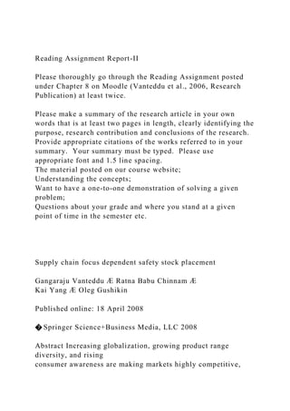
  • 40. performance. The different parameters for this serial supply chain are illustrated in Table 1. For the purpose of our discussion, we consider the player with no flexibility whatsoever with respect to its processing time as the bottleneck player. The effect of changing the position of the bottleneck player on the SC safety inventory costs is depicted below. We have considered three cases, wherein the processing time variability progressively increases (IV in Fig. 3), decreases (DV in Fig. 3), and remains constant (EV in Fig. 3) as we move from the most U/S stage to the most D/ S stage. For the increasing and decreasing cases, we kept the total processing 474 G. Vanteddu et al. 123 variability constant and progressively increased/decreased the process variability as we move from U/S to D/S in a symmetric fashion. When a particular stage is a
  • 41. bottleneck, the CIR for that particular stage would be unity and for all other stages the CIR is considered to be 0.9. Response related costs are not considered in the analysis as our primary intention is to show the effect of reducing the lead time on the safety stocks as the bottleneck player moves from U/S to D/S. By considering the incremental total supply chain safety stock costs with respect to a benchmark case, wherein all the players are operating at a CIR equivalent to 0.9 and the processing variability is the same at all the stages (as with the EV case in the chart), one can clearly see that the incremental total supply chain safety stock costs progressively increase as the bottleneck player moves from U/S to D/S for all three cases. Key managerial insight #1: Safety stock cost depends on the placement of the bottleneck player in a serial supply chain and it is desirable for the bottleneck player to be located towards the U/S rather than the D/S.
  • 42. 4.2 Safety stock costs versus responsiveness costs We illustrate the impact of CIR on the different cost curves in Fig. 4, using the cost expressions developed earlier. We know that, for any stage, safety stock related costs decrease (Eq. 15) and response related costs increase (Eqs. 17 and 18) with decrease in cycle time, or in Table 1 Parameters of the five- stage serial SC adopted for numerical analysis Stage/player 1 2 3 4 5 Nominal cumulative cost Cj 80 112 175 327 863 Average demand l 100 100 100 100 100 Demand variability r2 400 400 400 400 400 Mean processing time (periods) Lj 1 1 1 1 1 Processing variability ðl2r2j Þ (in number of units
  • 43. of product) 50 50 50 50 50 CIR cj 1 1 1 1 1 Safety coefficient kj 1.28 1.28 1.28 1.28 1.28 Average back order coefficient 0.1 0.1 0.1 0.1 0.1 Probability of stockout pj 0.1 0.1 0.1 0.1 0.1 Inventory holding cost hj 0.017 0.017 0.017 0.017 0.017 Service level U(kj) 0.9 0.9 0.9 0.9 0.9 External supplier Customer Supply Demand h i j lk Fig. 2 Schematic description of a serial supply chain Supply chain focus dependent safety stock placement 475 123 other words, with decrease in CIR. Hence, without loss of generality, we can say
  • 44. that the total cost function, which is a combination of safety stock and response related costs, tends to be convex, the optimum CIR shifting either towards or away from unity depending on whether responsiveness cost component or safety stock cost component is dominating. A very interesting result relevant to the nature of the total costs is due to Bookbinder and Cakanyildirim (1999), who show that the expected cost per unit time is jointly convex in the decision variables (Q,r,s), s being the expediting factor for a (Q,r) inventory system with expedited orders and random lead times. 4.3 Effect of cycle times and processing time variability on total stage cost Figure 5 illustrates the effect of increasing processing time variability at a particular stage on the total cost while keeping the other parameters constant. For the sake of numerical analysis, we have considered the parameter values for stage 3. PV in the chart stands for processing time variability and DV stands for demand variability.
  • 45. Increasing process variability tends to increase both the safety stock related costs and responsiveness related costs at different rates, primarily depending on the nominal cumulative cost Cj, the cost of volume flexibility function f(1 - cj), and the cost added at a stage (Cj - Ci). In the presence of increasing processing time variability, therefore, optimum CIR either moves away from or towards unity, -10 0 10 20 30 40 1 2 3 4 5 Supply Chain Bottleneck StageI nc re as e in
  • 46. T ot al S af et y St oc k C os t ( % ) IV EV DV Fig. 3 Incremental SC safety stock costs versus position of the bottleneck player 0 100 200 300
  • 47. 0.55 0.7 CIR C os t SS cost Response Cost Total Cost 10.85 Fig. 4 CIR versus stage costs 476 G. Vanteddu et al. 123 depending on whether safety stock cost component/or the responsiveness cost component is dominating. With increasing variability, the degree of departure of the optimum CIR value either way depends on the three factors mentioned above for a particular stage. To explain, to counter the excessive variability, a typical supply
  • 48. chain manager tries to reduce the cycle time (by reducing CIR), which would minimize the SS related costs. However, that action does not necessarily lead to reduction of the overall costs. For example, if the cost added at a particular stage is very high then the decrease in safety stock costs by cycle time reduction might not be able to offset the increase in cycle time reduction (responsiveness) costs. In such a scenario, moving CIR counterintuitively towards unity (i.e., increasing the cycle time), which means in the direction that increases safety stock costs, could be a better measure to reduce overall costs. Key managerial insight #2: As the processing time variability increases for a stage, the optimum value of CIR moves away from unity if safety stock cost component dominates the responsiveness cost component and towards unity if the responsiveness cost component dominates the safety stock cost component. In Fig. 5, optimum CIR is progressively moving away from unity as the PV/ DV ratio increases, because we have considered the safety stock
  • 49. costs component to be larger than the responsiveness cost component for our numerical analysis. The trend will be reversed if the response related costs dominate the safety stock related costs. In Fig. 5, for the case of PV/DV = 0.25, the optimum CIR value is 0.919, for which the respective safety stock and responsiveness cost components are $91.65 and $1.749 per period, respectively. For the case of PV/DV = 2, wherein the process variability increases eightfold compared to PV/DV = 0.25, the corresponding safety stock and responsiveness cost components are $138.6 and $1.75, respectively. In this case, not only is the safety stock component larger but also the effect of increasing process variability is much greater on safety stock component compared with responsiveness cost component. Hence, the optimum CIR value for the PV/DV = 2 case will move in the direction that will mitigate the effect of increasing safety stock costs and to a point where the
  • 50. cost advantage in terms of safety stock cost reduction by reducing the CIR is equalized by the corresponding increase in responsiveness costs. The optimum value for the PV/ DV = 2 case occurs at a CIR value of 0.909 (moving away from unity), with 50 150 250 350 0.55 0.7 0.85 CIR T ot al C os t PV/DV:0.25 PV/DV:0.5 PV/DV:0.75 PV/DV:1 PV/DV:1.5 PV/DV:2
  • 51. 1 Fig. 5 CIR versus total stage costs Supply chain focus dependent safety stock placement 477 123 corresponding safety stock and responsiveness cost components of $137.86 and $2.48, respectively. We extend the above analysis by performing a simple sensitivity analysis by considering the changes in mean processing time and nominal cost added at stage 3, while keeping other parameters constant. Table 2 presents the case with the mean processing time and nominal cost added both being halved. Table 3 presents the case with mean processing time and nominal cost added both being doubled. For the sake of simplicity, we have just considered the cases PV/DV = 0.25 and PV/DV = 2. For both of these cases, the optimum CIR for PV/DV = 2 occurs at a
  • 52. slightly lower value than that for PV/DV = 0.25 for the reasons mentioned in the preceding paragraph. The changes made in the parameter values are not able to make the responsiveness related costs increase at a faster rate than the decrease in safety stock related costs (with decreasing CIR), hence, the optimum CIR is still moving away from unity, primarily due to the parameter values we have assumed for our numerical analysis. We show in Sect. 4.4 that changes in the cost of flexibility function (COF), that is f(1 - cj), in our model cause the responsiveness related costs to increase at a faster rate than the decrease in safety stock related costs (with decreasing CIR), making the optimum CIR move towards unity. In a practical context, it all depends on the actual values of the parameters, which make either of the cost components dominating. The optimum value of the CIR for a stage will primarily depend upon the cumulative cost of the product, which in turn will depend upon the position of the
  • 53. stage in the supply chain, the cost added, and the nature of cost of volume flexibility function. Using the cycle time reduction as a lever may or may not be cost effective depending on, for example, whether a windscreen wiper is being assembled or an engine is being assembled at a stage. For the same cost of volume flexibility function, it might be a good idea to reduce the cycle time if a windscreen wiper is being assembled as opposed to an engine. Irrespective of the component that is being assembled, this effect will be more pronounced D/S when compared to U/S because the cumulative cost of the product will progressively increase as we move D/S. Key managerial insight #3: To reduce the safety stock costs, reducing the cycle time is a better lever at downstream stages when compared to upstream stages for a given responsiveness cost, all other parameters being held constant. Key managerial insight #4: All other parameters being constant, for a given cycle time reduction, the cost of flexibility function has to be milder for a stage with
  • 54. high cost addition when compared to a stage with low cost addition, to justify savings in safety stock costs. Table 2 Sensitivity analysis 1 CIR PV/DV = 0.25 PV/DV = 2 1 69.869 103.747 0.9 68.432 100.405 0.8995 68.441 100.404 0.899 68.450 100.403 0.895 68.533 100.407 478 G. Vanteddu et al. 123 The insight from Ryu and Lee (2003) ‘‘that in order to attain greater savings from the symmetric cost scheme for the two suppliers, the investment cost for the supplier with the more unreliable lead time should be smaller’’ looks similar in essence to our key managerial insight 2, albeit in a different context. One of the key insights offered, that downstream lead times have a greater impact on
  • 55. system performance than upstream ones (Gallego and Zipkin 1999), is also similar in spirit to our research. 4.4 Effect of cost of volume flexibility on total stage cost Figure 6 illustrates the effect of cost of volume flexibility at a particular stage on the total cost while keeping the other parameters constant. For the sake of numerical analysis, we have once again considered the parameter values for stage 3. COF in the chart stands for cost of volume flexibility function mildness/steepness, when compared to a randomly chosen increasing convex function (COF: 1). In Fig. 6, as expected, optimum CIR is progressively moving towards unity as the COF increases. As opposed to processing time variability, which affects both the safety stock cost component and the responsiveness cost components, cost of flexibility affects only the responsiveness cost component. Intuitively speaking,
  • 56. given that the stage is not operating at optimal CIR, increasing the cost of flexibility makes a typical supply chain manager operate close to nominal cycle times (CIR close to unity), but going back to the example given earlier, if a windscreen wiper is being assembled, particularly at a D/S stage, it is quite likely that there will be significant savings in safety stock costs by reducing the cycle time (moving the CIR away from unity), overtaking the extra cost of responsiveness because of a steeper flexibility function. The opposite will be true, for example, if an engine is being assembled at a stage. Table 3 Sensitivity analysis 2 CIR PV/DV = 0.25 PV/DV = 2 1 132.232 202.513 0.95 129.834 198.290 0.93 129.952 197.664 0.92 129.952 197.664 0
  • 57. 500 1000 1500 2000 2500 0.55 0.7 0.85 CIR T ot al C os t COF:0.01 COF:0.1 COF:0.33 COF:1 COF:2 COF:5 COF:10 1 Fig. 6 CIR versus total stage costs Supply chain focus dependent safety stock placement 479 123
  • 58. Key managerial insight #5: Given that a stage is not operating at optimal CIR, as cost of volume flexibility function becomes steeper, the optimum value of CIR moves towards unity if the responsiveness costs segment dominates the safety stock cost segment, and vice versa. Key managerial insight #6: All other parameters being constant, for the same cost addition at a stage, cost of flexibility function has to be milder at U/S than D/S for a given amount of savings in safety stock costs. While our model assumes information symmetry, it is still applicable, including the managerial insights, in supply chains with information asymmetry. For example, in the presence of bullwhip effect attributable to information asymmetry or other related issues, demand variability will progressively increase as we move towards the upstream stages. It is still advisable that mitigating measures are put in place to reduce the causative factors of the bullwhip effect. In the absence of any mitigating measures, one could also consider the actual variability at different
  • 59. stages and still use the model. The effect will be to accentuate both the safety stock component and the responsiveness cost component as we proceed upstream. If the increase in the cost of responsiveness at a stage is significantly larger compared to the reduction in safety stock costs for unit processing time reduction, the optimum CIR will move towards unity. The opposite trend will be witnessed in the opposite case. The change in the optimum CIR value at downstream stages may also be significant because of larger cumulative costs and typically large amounts of cost addition, in spite of the effect of bullwhip effect being smaller compared to upstream stages. 5 Model usability for achieving strategic fit The model can be used primarily as a building block in any kind of supply chain network both to evaluate the performance of individual stages with respect to the key order winners, cost, and responsiveness, and to optimize the
  • 60. supply chain depending upon the focus within the cost-responsiveness spectrum. The results can be used to evaluate the gap between the individual business strategies of different stages and the supply chain strategy, so that appropriate actions can be taken to achieve the strategic fit. Once the supply chain design is completed and the network is in place, the model will be particularly useful for making strategic decisions with regard to the safety stock placement while considering a changeover or introducing a new product. 5.1 Performance evaluation Total safety stock related cost (safety stock cost and responsiveness cost) expression for all the stages (using Eq. 20) can be easily evaluated given the different parameter values and one can obtain the costs separately for safety stock holding and cycle time reduction (if so desired by a stage) and the expected cycle
  • 61. times assuming that all the stages operate without any coordination with respect to the overall supply chain strategy (that is, there is no central decision maker). This 480 G. Vanteddu et al. 123 will allow stages to evaluate their performance with regard to the key order winners of cost and responsiveness and facilitates their comparison to the internal performance benchmarks. For example, a particular stage may realize that better operations management practices that involve the reduction of waste (lean practices) that had been planned for are ineffectual. Hence, they may want to know what went wrong and implement appropriate corrective and preventive actions such that cost and cycle time reductions can be achieved without any major investments. 5.2 Optimization
  • 62. Now, assuming that there is a central decision making mechanism, which acts to coordinate the whole supply chain, the overall safety stock related cost expression for the supply chain (Eq. 21) can be optimized, say for the optimal CIR values at all the stages given the constraints on target supply chain cycle time, individual stages’ rates of production, service levels, inventories, cost of inventory holding, etc. The optimal costs (safety stock inventory and responsiveness) can be compared with the costs obtained assuming the absence of the central decision maker (as for performance evaluation explained in Sect. 5.1) to initiate necessary actions. We also offer a simple optimization example based on the parameter values presented in Table 1 that lend support to the managerial insights developed in Sects. 4.3 and 4.4. Figure 7 depicts the optimal CIR values under different scenarios considered in
  • 63. Sects. 4.3 and 4.4. The only constraint considered was 0 B cj B 1. The total cost function was optimized under different scenarios. SC: Standard cost of flexibility function for all stages and other parameter values as per Table 1. DC: Decreasing cost of flexibility function (i.e., the function becomes milder compared to the SC case as we move from U/S to D/S); stage 3’s cost of flexibility function remaining the same as in the SC case. Other parameters for all the other stages remain as in the SC case. IV: Progressively increasing process variability as we move from U/S to D/S. For stage 3, process variability remains the same as in the SC case. Other parameters for all the other stages remain as in the SC case. 0.86 0.88 0.9 0.92
  • 64. 0.94 0.96 0.98 1 1 2 3 4 5 Player C IR SC DC IV DV Fig. 7 Player versus optimal CIR Supply chain focus dependent safety stock placement 481 123 DV: Progressively decreasing process variability as we move from U/S to D/S. For stage 3, process variability remains the same as in the SC case. Other parameters
  • 65. for all the other stages remain as in the SC case. The results, as can be seen from Fig. 7, clearly reinforce the insights developed in the earlier sections. The shift in the optimum CIR value at stage 5 shows strong variability owing to the fact that cost added constitutes a significant portion of the cumulative cost at that stage, thereby increasing the cost of responsiveness significantly for the same cost of flexibility function when compared to other stages. The same is the case with stage 4, although on a reduced scale. Since stage 3 is the transition stage under different scenarios retaining the same parameter values as compared to the SC case, there is no perceptible change in the optimum CIR value. 5.3 Achieving strategic fit If the overall costs at a stage are increasing as a result of optimization to achieve the strategic supply chain objectives, when compared to the costs in the absence of a central decision maker, i.e., by following its independent
  • 66. business strategy, then, by devising a scheme for the sharing of the additional profits for the whole supply chain in an equitable fashion, say, through changing the contract structure, discounts or other incentives, efforts could be made to coordinate the individual business strategies with the supply chain strategy to achieve the strategic fit. One way of doing this is by considering the supply chain objectives at different levels, say, strategic, tactical, and operational levels, and performing a gap analysis Strategic Objective:Customer Satisfaction Tactical Objective:Total customer Cycle time Performance evaluation for a hypothetical supply chain: Cost Estimate(Cip) $25,000 $100,000 $50,000 $0 $25,000 $0 Sum(Cip) $200,000 Time Required in months (Tip) 2 12 3 0 3 0 Max (Tip) 12 Tier-3 Supplier Tier-2 Supplier
  • 67. Tier-1 Supplier Mfg Unit D.C Retail Unit 5 4 3 2 1 Cost Estimate(Cjp) $5,000 $15,000 $0 $0 $6,000 $0 Sum(Cjp) $26,000 Time Required in months (Tjp) 1 4 0 0 1 0 Max (Tjp) 4 5 4 3 2 1 Cost Estimate(Ckp) $5,000 $15,000 $2,000 $10,000 $6,000 $0 Sum(Ckp) $38,000 Time Required in months (Tkp) 2 2 1 1 1 0 Max (Tkp) 2
  • 68. 5 4 3 2 Overall cost= 1 Sum(Sum(Cip)+ …+Sum(Ckp)) $264,000 Max(T) : Max(max(Tip),max(Tjp),max(Tkp)) 12 NC product level Throughput rate Information symmetry level P E R F O R M A
  • 69. N C E M E T R IC S Fig. 8 Performance comparison for different players in a supply chain (adopted from Vanteddu et al. 2006) 482 G. Vanteddu et al. 123 between the individual business strategies and the supply chain strategy in terms of costs and responsiveness. Vanteddu et al. (2006) offers a simple Excel based model to achieve strategic fit assuming that quantitative data is available to make use of the tool, as illustrated in Fig. 8.
  • 70. By simply modifying the performance metrics by placing emphasis on cost efficiency and responsiveness, one can use the above model to achieve the strategic fit. Actual costs related to cost and responsiveness can be obtained by using the model proposed in this paper. 6 Conclusions In this paper, in addition to offering several managerial insights with regard to strategic safety stock placement in a supply chain, an attempt has been made to address the problem of achieving compatibility between the supply chain strategy and the individual stage’s business strategy by primarily considering safety stocks and responsiveness related costs. We introduce a new parameter called the coefficient of inverse responsiveness (CIR) to model response related costs at a stage, which also enhances the scalability of the model. The developed cost function for the building block could be easily extended for any type of supply chain
  • 71. network. By knowing the values of the parameters of the model, one can know the safety stock costs and responsiveness related costs at each stage and compare them to an ideal supply chain strategy in terms of cost and responsiveness to make informed decisions. The key managerial insights developed are generic in nature and applicable to any supply chain irrespective of its placement on the cost- responsiveness spectrum and topology. To make the model more tractable we had to make certain simplifying assumptions and following are some of the limitations related to those assumptions. For example, we did not factor the bullwhip effect into our model. It would be an interesting extension to our research if the bullwhip effect and other information asymmetry related issues were factored into the model. We have not incorporated order sizes into our model because the model is supposed to be largely a strategic
  • 72. model. Research could be extended by incorporating this aspect into the model to see how it affects the managerial insights that we offered. Relaxing the assumptions on the stationary nature of the demand and stage base stock policy with periodic review will make the model more realistic and robust to real- world situations. Introducing contracts that affect the flexibility at a stage with financial ramifications will also be a very fertile area to pursue that will make our model mimic reality more closely. Another such area is the consideration of other types of network topologies, particularly assembly and distribution; we are planning to consider extension of the framework in this direction. It would also make more sense to consider capacity constraints at certain stages. Product mix related flexibility is also a crucial factor which is not addressed in our model. Addition of this feature would truly make the research more in tune with reality, especially in mass customization
  • 73. settings. Finally, we really would like to see this model used in some real-world application so that insights presented in our model could be validated. Supply chain focus dependent safety stock placement 483 123 References Axsäter S (1993) Continuous review policies for multi-level inventory systems with stochastic demand. In: Graves S, Rinnooy Kan A, Zipkin P (eds) Logistics of production and inventory. Elsevier Science, North Holland Axsäter S, Rosling K (1993) Notes: installation vs. Echelon stock policies for multilevel inventory control. Manage Sci 39(10):1274–1280 Ben-Daya M, Raouf A (1994) Inventory models involving lead time as decision variables. J Oper Res Soc 45:579–582 Bookbinder JH, Cakanyildirim M (1999) Random lead times and expedited orders in (Q, r) inventory systems. Eur J Oper Res 115:300–313
  • 74. Cherukuri SS, Nieman RG, Sirianni NC (1995) Cycle time and the bottom line. Indust Eng 27(3):20–23 Choi JW (1994) Investment in the reduction of uncertainties in just in time purchasing systems. Naval Res Logistics 41:257–272 Chopra S, Meindl P (2004) Supply chain management: strategy, planning and operation, 2nd edn. Pearson Education Inc., Upper Saddle River Chopra S, Reinhardt G, Dada M (2004) The effect of lead time uncertainty on safety stocks. Decis Sci 35(1):1–24 Clark A, Scarf H (1960) Optimal policies for a multi echelon inventory problem. Manage Sci 6:474–490 Davis D, Buckler J, Mussomeli A, Kinzler D (2005) Inventory transformation: Revlon style. Supply Chain Manage Rev 9(5):53–59 Eppen GD, Martin RK (1988) Determining safety stock in the presence of stochastic lead time and demand. Manage Sci 34(11):1380–1390 Ettl M, Feigin GE, Lin GY, Yao DD (2000) A supply network model with base—stock control and service requirements. Oper Res 48:216–232
  • 75. Felgate R, Bott S, Harris C (2007) Get your timing right. Supply Manage 12(1):17 Feller W (1960) An introduction to probability theory and its applications, vol I. Wiley, New York Fisher ML (1997) What is the right supply chain for your product? Harv Bus Rev 75(2):105–116 Gallego G, Zipkin P (1999) Stock positioning and performance estimation in serial production- transportation systems. Manuf Serv Oper Manage 1(1):77–88 Gaur V, Giloni A, Seshadri S (2005) Information sharing in a supply chain Under ARMA demand. Manage Sci 51(6):961–969 Glasserman P, Tayur S (1995) Sensitivity analysis for base stock levels in multi echelon production- inventory system. Manage Sci 41:216–232 Glasserman P, Tayur S (1996) A simple approximation for a multi stage capacitated production inventory systems. Naval Res Logistics 43:41–58 Graves S (1985) Multi echelon inventory model for a repairable item with one for one replenishment. Manage Sci 31:1247–1256 Graves SC (1988) Safety stocks in manufacturing systems. J
  • 76. Manuf Oper Manage 1:67–101 Graves SC, Willems SP (2003) Supply chain design: safety stock placement and supply chain configuration. In: de Kok AG, Graves SC (eds) Handbooks in operations research and management science, supply chain management: design, coordination and operation, Chap 3, vol 11. Elsevier BV, Amsterdam, The Netherlands Hanssmann F (1959) Optimal inventory location and control in production and distribution networks. Oper Res 7:483–498 Hill T (1993) Manufacturing strategy: text and cases, 2nd edn. IRWIN, Illinois Kapuscinski R, Tayur S (1999) Optimal policies and simulation based optimization for capacitated production inventory systems. In: Tayur S, Ganeshan R, Magazine MJ (eds) Quantitative models for supply chain management. Kluwer Academic Publishers, Boston Lee HL, Billington C (1993) Material management in decentralized supply chains. Oper Res 41(5):835– 847 Lee HL, Moinzadeh K (1987a) Two parameter approximations for multi echelon repairable inventory
  • 77. models with batch ordering policy. IIE Trans 19:140–149 Lee HL, Moinzadeh K (1987b) Operating characteristics of a two echelon inventory system for repairable and consumable items under batch ordering and shipment policy. Naval Res Logistics Quart 34:365–380 Lee Y, Zipkin P (1992) Tandem queues with planned inventories. Oper Res 40:936–947 484 G. Vanteddu et al. 123 Moon I, Choi S (1998) Technical note: a note on lead time and distributional assumptions in continuous review inventory models. Comput Oper Res 25(11):1007–1012 Nazzal D, Mollaghasemi M, Anderson D (2006) A simulation- based evaluation of the cost of cycle time reduction in Agere systems wafer fabrication facility—a case study. Int J Prod Econ 100:300–313 Rosling K (1989) Optimal inventory policies for assembly systems under random demands. Oper Res 37:565–579
  • 78. Ryu SW, Lee KK (2003) A stochastic inventory model of dual sourced supply chain with lead-time reduction. Int J Prod Econ 81–82:513–524 Simchi-Levi D, Zhao Y (2005) Safety stock positioning in supply chain with stochastic lead times. Manuf Serv Oper Manage 7(4):295–318 Simpson KF (1958) In process inventories. Oper Res 6:863–873 Sourirajan K, Ozsen L, Uzsoy R (2007) A single-product network design model with lead time and safety stock considerations. IIE Trans 39:411–424 Speck C, vander Wal J (1991) The capacitated multi echelon inventory system with serial structure: 1. The ‘‘push-ahead’’ effect. Memorandum COSOR 91-39, Eindhoven University of Technology, Eindhoven, The Netherlands Upton DM (1997) Process range in manufacturing: an empirical study of flexibility. Manage Sci 43(8):1079–1092 Van Houtum GJ, Inderfurth K, Zijm WHM (1996) Materials coordination in stochastic multi echelon systems. Eur J Oper Res 95:1–23 Vanteddu G, Chinnam RB, Yang, K (2006) A performance
  • 79. Comparison tool for Supply Chain management. Int J Logistics Syst Manage 2(4):342–356 Yang B, Geunes J (2007) Inventory lead time planning with lead-time sensitive demand. IIE Trans 39(5):439 Supply chain focus dependent safety stock placement 485 123 Supply chain focus dependent safety stock placementAbstractIntroductionLiterature reviewModel developmentExpression for safety stock costsExpression for responsiveness related costsDirect responsiveness related costsIndirect responsiveness related costsManagerial insights for strategic safety stock placementPosition of the bottleneck playerSafety stock costs versus responsiveness costsEffect of cycle times and processing time variability on total stage costEffect of cost of volume flexibility on total stage costModel usability for achieving strategic fitPerformance evaluationOptimizationAchieving strategic fitConclusionsReferences << /ASCII85EncodePages false /AllowTransparency false /AutoPositionEPSFiles true /AutoRotatePages /None /Binding /Left /CalGrayProfile (None) /CalRGBProfile (sRGB IEC61966-2.1) /CalCMYKProfile (ISO Coated v2 300% 050ECI051) /sRGBProfile (sRGB IEC61966-2.1) /CannotEmbedFontPolicy /Error /CompatibilityLevel 1.3
  • 80. /CompressObjects /Off /CompressPages true /ConvertImagesToIndexed true /PassThroughJPEGImages true /CreateJDFFile false /CreateJobTicket false /DefaultRenderingIntent /Perceptual /DetectBlends true /ColorConversionStrategy /sRGB /DoThumbnails true /EmbedAllFonts true /EmbedJobOptions true /DSCReportingLevel 0 /SyntheticBoldness 1.00 /EmitDSCWarnings false /EndPage -1 /ImageMemory 524288 /LockDistillerParams true /MaxSubsetPct 100 /Optimize true /OPM 1 /ParseDSCComments true /ParseDSCCommentsForDocInfo true /PreserveCopyPage true /PreserveEPSInfo true /PreserveHalftoneInfo false /PreserveOPIComments false /PreserveOverprintSettings true /StartPage 1 /SubsetFonts false /TransferFunctionInfo /Apply /UCRandBGInfo /Preserve /UsePrologue false /ColorSettingsFile () /AlwaysEmbed [ true ]
  • 81. /NeverEmbed [ true ] /AntiAliasColorImages false /DownsampleColorImages true /ColorImageDownsampleType /Bicubic /ColorImageResolution 150 /ColorImageDepth -1 /ColorImageDownsampleThreshold 1.50000 /EncodeColorImages true /ColorImageFilter /DCTEncode /AutoFilterColorImages false /ColorImageAutoFilterStrategy /JPEG /ColorACSImageDict << /QFactor 0.76 /HSamples [2 1 1 2] /VSamples [2 1 1 2] >> /ColorImageDict << /QFactor 0.76 /HSamples [2 1 1 2] /VSamples [2 1 1 2] >> /JPEG2000ColorACSImageDict << /TileWidth 256 /TileHeight 256 /Quality 30 >> /JPEG2000ColorImageDict << /TileWidth 256 /TileHeight 256 /Quality 30 >> /AntiAliasGrayImages false /DownsampleGrayImages true /GrayImageDownsampleType /Bicubic /GrayImageResolution 150 /GrayImageDepth -1 /GrayImageDownsampleThreshold 1.50000
  • 82. /EncodeGrayImages true /GrayImageFilter /DCTEncode /AutoFilterGrayImages true /GrayImageAutoFilterStrategy /JPEG /GrayACSImageDict << /QFactor 0.76 /HSamples [2 1 1 2] /VSamples [2 1 1 2] >> /GrayImageDict << /QFactor 0.15 /HSamples [1 1 1 1] /VSamples [1 1 1 1] >> /JPEG2000GrayACSImageDict << /TileWidth 256 /TileHeight 256 /Quality 30 >> /JPEG2000GrayImageDict << /TileWidth 256 /TileHeight 256 /Quality 30 >> /AntiAliasMonoImages false /DownsampleMonoImages true /MonoImageDownsampleType /Bicubic /MonoImageResolution 600 /MonoImageDepth -1 /MonoImageDownsampleThreshold 1.50000 /EncodeMonoImages true /MonoImageFilter /CCITTFaxEncode /MonoImageDict << /K -1 >> /AllowPSXObjects false /PDFX1aCheck false /PDFX3Check false
  • 83. /PDFXCompliantPDFOnly false /PDFXNoTrimBoxError true /PDFXTrimBoxToMediaBoxOffset [ 0.00000 0.00000 0.00000 0.00000 ] /PDFXSetBleedBoxToMediaBox true /PDFXBleedBoxToTrimBoxOffset [ 0.00000 0.00000 0.00000 0.00000 ] /PDFXOutputIntentProfile (None) /PDFXOutputCondition () /PDFXRegistryName (http://www.color.org?) /PDFXTrapped /False /Description << /ENU <FEFF004a006f0062006f007000740069006f006e007300200066 006f00720020004100630072006f0062006100740020004400690 07300740069006c006c0065007200200036002e000d0050007200 6f006400750063006500730020005000440046002000660069006 c0065007300200077006800690063006800200061007200650020 007500730065006400200066006f0072002000640069006700690 0740061006c0020007000720069006e00740069006e0067002000 61006e00640020006f006e006c0069006e0065002000750073006 100670065002e000d002800630029002000320030003000340020 0053007000720069006e00670065007200200061006e006400200 049006d007000720065007300730065006400200047006d006200 48> /DEU <FEFF004a006f0062006f007000740069006f006e007300200066
  • 84. 006f00720020004100630072006f0062006100740020004400690 07300740069006c006c0065007200200036002e000d0050007200 6f006400750063006500730020005000440046002000660069006 c0065007300200077006800690063006800200061007200650020 007500730065006400200066006f00720020006f006e006c00690 06e0065002e000d00280063002900200032003000300038002000 53007000720069006e006700650072002d005600650072006c006 1006700200047006d006200480020000d000d0054006800650020 006c00610074006500730074002000760065007200730069006f0 06e002000630061006e00200062006500200064006f0077006e00 6c006f00610064006500640020006100740020006800740074007 0003a002f002f00700072006f00640075006300740069006f006e0 02e0073007000720069006e006700650072002e0063006f006d00 0d0054006800650072006500200079006f0075002000630061006 e00200061006c0073006f002000660069006e0064002000610020 007300750069007400610062006c006500200045006e0066006f0 063007500730020005000440046002000500072006f0066006900 6c006500200066006f0072002000500069007400530074006f007 0002000500072006f00660065007300730069006f006e0061006c 0020003600200061006e0064002000500069007400530074006f0 07000200053006500720076006500720020003300200066006f00 7200200070007200650066006c00690067006800740069006e006 700200079006f007500720020005000440046002000660069006c 006500730020006200650066006f007200650020006a006f00620 020007300750062006d0069007300730069006f006e002e> >> >> setdistillerparams << /HWResolution [2400 2400] /PageSize [5952.756 8418.897] >> setpagedevice