This document presents a methodology for numerically predicting Nusselt number equations for stirred tanks with helical coils using computational fluid dynamics (CFD). The approach uses a validated CFD model to obtain heat transfer coefficients, which has advantages over experimental methods by allowing testing of different configurations without physical experiments. A literature review covers previous experimental and numerical studies on heat transfer in stirred tanks. Key factors in CFD simulations like mesh refinement, discretization schemes, turbulence models, and approaches to model impeller-baffle interaction are discussed. The methodology is illustrated by comparing a generated Nusselt number correlation to experimental data with an average 10.7% deviation.

1. PROCESS SYSTEMS ENGINEERING
Numerical Prediction of a Nusselt Number Equation
for Stirred Tanks with Helical Coils
Ronald Jaimes Prada and Jos
e Roberto Nunhez
School of Chemical Engineering, University of Campinas, Albert Einstein Avenue 500.
Campinas 13083-970, Brazil
DOI 10.1002/aic.15765
Published online in Wiley Online Library (wileyonlinelibrary.com)
A methodology to obtain a Nusselt correlation for stirred tank reactors is presented. The novelty of the approach is the
use of a validated computational model to obtain the heat-transfer coefficients. The advantages of this new approach
are many, including the possibility of testing different heat-transfer configurations to obtain their Nusselt correlation
without performing experimental runs. Physical phenomena involved was represented both qualitatively and quantita-
tively. The classical experimental work of (Oldshue and Gretton, Chem Eng Prog. 1954;50(12):615–621) illustrates the
procedure. A sufficient number of virtual points in the whole range of the Reynolds number should be obtained. Results
strongly depend on mesh refinement in the boundary layer, so a procedure is suggested to guarantee heat-transfer coef-
ficients are accurately estimated. The final Nusselt correlation was compared against all the 107 experimental points of
the work by (Oldshue and Gretton, Chem Eng Prog. 1954;50(12):615–621), and an average deviation on the results of
10.7%. V
C 2017 American Institute of Chemical Engineers AIChE J, 00: 000–000, 2017
Keywords: convective heat transfer, stirred tank reactors, helical coils, computational fluid dynamics
Introduction
Stirred tank reactors are processing units used in different
industrial operations with the purpose of obtaining a homoge-
neous mixture and uniform heat and mass transfer throughout
the vessel.1
Crystallization, liquid-liquid extraction, leaching,
heterogeneous catalytic reactions, and fermentation are some
examples of operations that are carried out in this type of reac-
tor. To ensure homogenization, one or more impellers are used
to generate the desired flow and mixing within these devices.
In reactions where the optimal temperature condition is not
reached, heating or cooling of the system is necessary to
increase the efficiency of the reaction or, in some cases, to
ensure the safety of the operation. To keep the fluid in the
reactor at the desired temperature, heat must be added or
removed by a jacket on the tank wall and/or through coils
(axial or helical) immersed in the fluid, aiming to promote
heat transfer. The heat-transfer rate added or removed depends
on the physical properties of the fluids (the bulk fluid and the
fluid used for heat exchange), geometric parameters, and the
degree of agitation. A large number of correlations were pro-
posed in the literature for the estimation of the process-side
heat-transfer coefficient, and most of them are expressed of
the form2
Nu5KðReÞa
ðPrÞb
ðlRÞc
ðGcÞ (1)
Where Re is the Reynolds number, Pr is the Prandtl number,
lR 5 lw
l is the viscosity ratio. lw is the value of the viscosity
at the wall and l is the bulk viscosity, K, a, b, and c are
constants and (Gc) represents a geometry correction. Most
researchers recommend values of 2/3 for the exponent of the
Reynolds number (a), 1/3 for the exponent of the Prandtl num-
ber (b), and 0.14 for the exponent of the viscosity ratio (c).
The value of the constant (K) depends on the type of impeller
and heat-transfer surface, taking values from 0.3 to 1.5. All of
the above constants are experimentally evaluated and the gen-
erated correlation can only be applied when there is geometric
similarity. To increase the range of validity of the correlation
for a wider range of geometries, some researchers have incor-
porated dimensionless geometric relations (Gc).3
Chilton et al.4
conducted the first study of the film coeffi-
cient in stirred tanks with helical coils using the flat paddle
impeller. A correlation for forced convection heat transfer was
proposed. The vessel diameter was used in the Nusselt number
h D
k
instead of the coil diameter, h d
k
, as most works do. In
these two equations k is the thermal conductivity of the fluid,
h is the heat-transfer coefficient, and D and d are the impeller
and coil diameters, respectively. Four fluids were used (water,
two oils, and glycerol) and the temperature difference across
the heat-transfer surface was varied over a wide range.
Pratt5
developed correlations for the outer (ho) and inner
(hi) heat-transfer coefficient in square and cylindrical stirred
vessels. These devices were equipped with helical coils and
flat paddle impellers. In this study, the influence of the coil
geometry was analyzed incorporating some parameters in the
correlation, such as the diameter and total height of the coil.
The authors concluded that due to the operating range of the
tests (Reynolds number varied from 18.800 to 513.000), a
lower exponent (close to 0.5) for the Reynolds number was
Correspondence concerning this article should be addressed to R. P. Jaimes at
ronaldjaimes@gmail.com (or) J. R. Nunhez at nunhez@feq.unicamp.br.
V
C 2017 American Institute of Chemical Engineers
AIChE Journal 1
2017 Vol. 00, No. 00

2. obtained, when compared to the general value of 2/3 in most
correlations presented in the literature.
Cummings and West6
extended the correlation reported by
Chilton et al.4
to apply it in the study of larger stirred tanks.
Their experiments included six different liquids with different
physical and thermal properties: water, toluene, isopropyl
alcohol, ethylene glycol, glycerol, and mineral oil and two
types of impeller: retreating-blade and 45 pitched blade tur-
bine impeller (PBT).
Oldshue and Gretton7
studied the heat-transfer coefficient
for stirred tanks with helical coils and baffles on the tank wall.
The effect of the variation of both the impeller (Rushton
impeller, called flat-blade turbine impeller in the paper) and
coil diameters have been studied for heating and cooling. A
range of Reynolds number from 400 to 1.5 3 106
was used.
When the results of these experiments were compared to pre-
vious works, it was clear that it was necessary to include other
parameters in the correlation to obtain a better understanding
of the heat-transfer process. It should be pointed out that
researchers using a tube of larger diameter automatically
obtained a higher Nusselt number for the same Reynolds num-
ber. Furthermore, the use of an impeller with higher power
consumption at a given Reynolds number provides a higher
coefficient of heat transfer due, primarily, to the higher energy
input.
Appleton and Brennan8
studied the effect of the impeller
design, the geometry and the roughness of the coil surface, as
well as the type of the coil arrangement (baffle and helical
coils) to estimate the heat-transfer coefficient for flat bottomed
tanks. The authors worked on a wide range of Prandtl and
Reynolds numbers. They reported that the heat-transfer coeffi-
cient is increased when finned tubes are used.
Jha and Rao9
predicted the Nusselt number based on the
helical coil geometry and the impeller location within the tank
for several configurations.
Nagata et al.10
determined correlations of the heat-transfer
coefficient for a cooling jacket (hj) and a rotating coil acting as
an impeller (hc), working with highly viscous non-Newtonian
fluids in laminar and turbulent flow. They observed that the hc
coefficient is approximately three times greater than the hj
coefficient due to a higher local shear rate outside the coil sur-
face, which promotes heat transfer. In addition, the lower
apparent viscosity of the pseudoplastic and Bingham fluids
increase heat transfer.
Havas et al.11
studied the heat-transfer coefficient in a
stirred tank using vertical tube baffles. They introduced a mod-
ified Reynolds number in the heat-transfer equation and
reported that this modified number is suitable for obtaining a
better prediction of the heat-transfer coefficients for different
coil geometries. Furthermore, they showed that this modified
Reynolds number is also suitable for predicting the heat-
transfer coefficients in helical coils. The experimental data
showed that the effect of the baffles on the heat transfer is sig-
nificant in these devices.12
Karcz and Strek13
studied the effect of the geometric param-
eters of the baffles on the heat-transfer coefficient. These
experiments were carried out in a jacketed stirred tank for
three different impellers (Rushton turbine, pitched-blade, and
a propeller). The authors, different from the results obtained
by Havas et al.12
(for systems with helical coils), found that
the geometric parameters of the baffles have a significant
effect on the heat-transfer coefficient in jacketed stirred tanks
equipped with high speed impellers.
Perarasu et al.14
studied a stirred tank equipped with coils
using two types of impellers (propeller and disk turbine)
with a heat input variation. The authors found that the effect
of the heat input in the heat-transfer coefficient changes
with the type of impeller. At a given speed, the heat-transfer
coefficient of the disk turbine impeller increases with
increasing heat input, while for the propeller impeller the
heat-transfer coefficient increases to a certain point, and
then, it decreases. Empirical correlations proposed by the
authors fit the experimental data in a range of 615% for
the two impellers.
Experimental studies have the advantage of dealing with the
real configuration. However, physical experiments can be
expensive and time consuming. Furthermore, full-scale experi-
mentation cannot often be performed for large systems or sys-
tems involving dangerous materials. Computational Fluid
Dynamics (CFD) is an alternative technique that can be used
to reduce cost and provide support for the analysis of mixing
processes. This technique provides a detailed description of
the flow, enabling a better understanding of the phenomena
involved. The advantages of this numerical technique are a
substantial reduction of time in most cases; the possibility to
study systems where controlled experiments are very difficult
to be performed (large systems or systems involving hazard-
ous materials), and the achievement of results in a nonintru-
sive way.
In general, CFD allows a better understanding of the flow
which in turn, allows the optimization of processes. It can also
help experimental research to be more efficient. The CFD sim-
ulation models in mixing tanks require an appropriate resolu-
tion of the mesh, the use of a good discretization scheme, a
right choice for the turbulence model, and a suitable approach
to represent the impeller-baffle interaction. The selection of
the numerical considerations mentioned above can have a
marked influence on both the accuracy of the results and the
computational cost.15
Computational mesh resolution is an important factor in any
CFD simulation and is directly associated with the computing
time. To obtain a mesh with a good accuracy in the results, at
a reasonable computational cost, it is necessary to carry out
simulations with different mesh densities until constant values
of the interested variables are reached. More details on how
the mesh refinement should be carried out is given in section
“Mesh refinement.”
Many authors have studied the effect of the discretization
scheme on the accuracy of the flow pattern in mixing tanks.
Sahu and Joshi16
used the IBM technique (Impeller Boundary
Conditions) to simulate a pitched blade turbine (PBT) and
compared three different discretization schemes of first order
(Upwind, Upwind-central differences, and the power law
scheme). The authors noted that the Upwind discretization
scheme showed significant differences compared with the
other two schemes, which showed similar results, although
the Upwind scheme converged more quickly. The schemes
were evaluated with experimental data, and it was claimed
that the power law scheme is more robust and has greater
accuracy.
Brucato et al.17
compared the hybrid central difference
scheme to the high-order discretization scheme Quadratic
Upstream Interpolation (QUICK). They observed that the flow
fields have no significant difference between the two discreti-
zation schemes, however, the QUICK numerical scheme tends
to reproduce slightly higher recirculation rates at the top and
2 DOI 10.1002/aic Published on behalf of the AIChE 2017 Vol. 00, No. 00 AIChE Journal

3. bottom of the tank. Moreover, it was observed that the effects
of numerical diffusion associated with the Upwind scheme
were not significant for very fine meshes, and the turbulent dif-
fusion was highly dominant.
Aubin et al.18
studied the effect of three discretization
schemes (Upwind, Upwind-central differences, and QUICK)
and verified that the choice of the discretization scheme has
little effect on the average speed (in agreement with the results
obtained by Brucato et al.17
). They noticed an underestimation
of the vortex in the region below the impeller, which is related
to the use of RANS turbulence models.
Different approaches have been developed to describe the
interaction impeller-baffle in CFD simulations. These
approaches can be classified into two categories: steady-state
and transient-state. In the first category, the model equations
are solved in steady-state and in the second category the inter-
actions impeller-fluid are modeled in a time dependent fash-
ion.19,20
These approaches may include impeller boundary
conditions (IBC), specification of source-sink terms (source
terms for the blades and sink terms for the baffles) or incorpo-
rating rotating and stationary frames. Out of these, two
approaches are commonly used: Multiple Frames of Reference
(MFR) and sliding mesh (SM). According to some authors, the
MFR approach21
provides suitable results with a smaller com-
putational cost compared to other transient approaches to sim-
ulate stirred tanks.15,17,18,22
The turbulence model k- is the most used for CFD simu-
lations in mixing tanks. In most of these studies, the model
showed deficiencies in the prediction of the turbulent quanti-
ties due to the assumption of isotropic turbulence, limiting
the prediction of vortices or recirculating flows.23–25
The
prediction of the flow in mixing tanks has been studied
by several authors, using variations of the k– model such
as Chen Kim and the Renormalization Group (RNG)
model.18,25–27
Jaworski et al.28
studied the flow produced by Rushton
impellers using the sliding mesh approach. They reported that
the choice of the turbulence model does not have much influ-
ence on the average speeds. The turbulent quantities were
highly underestimated by the two models. However, the stan-
dard k– model showed better results in comparison to the
RNG k– model.
Bakker et al.29
investigated laminar and turbulent flow pat-
terns for a pitched blade impeller (PBT) with four blades,
using three turbulence models (standard k–, RNG k–, and
RSM models). The authors showed that the axial-radial veloc-
ity field predicted by the three models presented similar results
in comparison with the experimental data. Predictions of the
turbulent dissipation were marginally different for the three
models. Sheng et al.30
also predicted the flow pattern for a
PBT impeller with four blades, using the RNG k– and RSM
models. As previous authors, they found a good prediction of
the average velocity field in comparison with experimental
data obtained by Particle Image Velocimetry (PIV) technique
and Laser-Doppler Velocimetry (LDV), but the turbulent
quantities were underestimated.
Oshinowo et al.31
studied the effect of standard turbulence
models k–, RNG k–, and RSM in the tangential velocity
field using the MFR approach. They found inverted vortex
regions in the top of the tank which are not according to the
physical phenomenon. This problem can be minimized
through the use of the RNG and RMS models, this last one
being even more effective.
Montante et al.32
simulated mixing tanks equipped with
Rushton type impellers using the Slind Grid (SG), and Inner-
outer iterative procedure (IO) approaches. Initially the SG
technique had a part of its mesh moving (where the impeller is
located) with the speed of the impeller. The mesh layer at the
interface of the static and moving mesh is continually chang-
ing due to the movement of the impeller. More details are
found in Murthy et al.33
The simulations were compared with
experimental data obtained by Laser-Doppler Anenometry
(LDA) technique and showed a correct prediction of the flow
pattern transition as well as the C/T values at which the transi-
tion occurs.
Aubin et al.18
conducted studies on the turbulence models
k– and RNG k– regarding the average velocities, turbulent
kinetic energy, and global quantities such as power and pump-
ing numbers. They found no significant effects in the axial and
radial velocity fields or the inverted tangential movement in
the upper part of the vessel, differently from what was
observed by Oshinowo et al.31
Spogis and Nunhez34
used the Shear Stress Transport (SST)
turbulence model, which is a mixture of both the k– and k–x
models. They reported the turbulence model was able to cor-
rectly estimate the turbulence quantities for both a modified
PBT impeller and a hydrofoil they proposed.
This work aims at proposing a CFD model able to obtain
with accuracy the process side heat-transfer coefficient of a
stirred tank with internal helical coils and stirred by a Rush-
ton Impeller. All modeling aspects mentioned above are
important to obtain a good CFD model. However, as the
main prediction of this work is the estimation of the heat-
transfer coefficient, additional aspects have to be considered
in the model, which will be detailed in the model description.
A methodology is also proposed for the obtaining of the film
coefficients and the development of a Nusselt equation based
on numerical simulation. The obtained model was compared
to the data obtained by Oldshue and Gretton7
with good accu-
racy, as will be shown in the results section. The advantages
of this new approach are many, including the possibility of
using a different heat-transfer configuration to obtain the
Nusselt correlation without the need of performing experi-
mental runs for the new geometry, which would require a
need to build a new equipment and run experiments to obtain
a new Nusselt correlation. Also, as CFD is able to evaluate
locally the characteristics of the process, this new approach
can help optimize the equipment by improving on regions
where heat transfer is poor.
Methodology
To describe the physical phenomena in the stirring and mix-
ing processes, the mass conservation of the fluid was modeled
by Eq. 2. The momentum conservation (Eq. 3) used the
Navier-Stokes Equations and the heat transfer was accounted
for by the conservation of energy (Eq. 4). These equations
were applied to an incompressible flow.
Mass conservation
@vi
@xi
1
@vj
@xj
1
@vk
@xk
50 (2)
where vi, vj, and vk are the velocities in the i, j, and k
directions.
AIChE Journal 2017 Vol. 00, No. 00 Published on behalf of the AIChE DOI 10.1002/aic 3

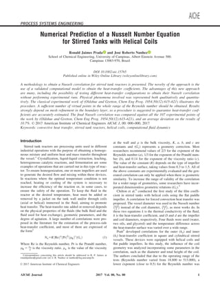
4. Momentum conservation
q
@vi
@t
1vi
@vj
@xj
52
@p
@xi
1leff
@2
vi
@xj
2
1qgi1
X
Fi (3)
where q is the density, p is the pressure, leff is the effective
viscosity (leff 5 lf 1 lt), l is the kinematic viscosity, lt is the
turbulent viscosity, gi is the gravitational acceleration in the i
direction,
P
Fi is the source term due to both the centrifugal
and Coriolis forces. The SST turbulent kinetic energy k is
derived from the Boussinesq hypothesis and is defined in
terms of velocity fluctuations. and x are both used depending
on the proximity of the walls and it is automatically set by the
SST model. More details on the turbulence model and how
this viscosity is related to the turbulent energy and its dissipa-
tion is found in Menter.35,36
Energy conservation
@ qE
ð Þ
@t
1
@ vi qE1p
ð Þ
½
@xi
5
@
@xi
keff
@T
@xi
2
X
j0
hj0 Jj0;i1vj sij
eff
2
4
3
51Sh
(4)
where E is the energy, which is related to the static enthalpy h,
T is the temperature, keff is the effective thermal conductivity
of the fluid (keff 5 kf 1 kt), kf is the thermal conductivity of
the fluid and kt is the turbulent thermal conductivity of the
fluid, Jj0
;i is the i component of the diffusion flux of species j0
in the mixture and includes a turbulent diffusion term in turbu-
lent flows, sij
eff
is the stress tensor, a collection of velocity
gradients that represent heat losses through viscous dissipation
and Sh is a general source term. More details are found in
chapter 5 of Paul et al.37
Stirred Tank Configuration. Steady-state heat-transfer
numerical experiments were carried out in a flat-bottom cylin-
drical vessel with four equally spaced baffles located perpen-
dicular to the tank wall, as shown in Figure 1. Stirring is
provided by a standard six-bladed Rushton turbine impeller
and a set of helical coils distributed along its length has been
selected as heat exchange internal devices, following the
experimental arrangement by Oldshue and Gretton.7
The
diameters of the Rushton turbine impellers (D) are the same
used in the experimental tank (0.30 m, 0.41 m, 0.51 m, 0.61
m, and 0.71 m). Oldshue and Gretton7
used two coil diameters
(d) of 0.022 m and 0.044 m, which was also used in the
numerical model. Following the experiments, the impellers
and the coils were located at a distance of the tank bottom (Cc)
of 0.41 m and 0.18 m, respectively. Table 1 contains the geo-
metric parameters used in all cases studied, which were based
on the experimental work by Oldshue and Gretton.7
To obtain
steady-state conditions, alternate coils were used for heating
and cooling with adiabatic tank wall, similar to what was used
in the experimental work. The two coils have outside diame-
ters of 0.91 m and 0.455m. According to Oldshue and Gret-
ton,7
these diameters are about as large and as small as would
be practical. The pitch (Sc) for the larger diameter is 0.0889 m
and 0.0445 for the smaller tube. The dimensions of these coils
are shown in Table 2 where Do (m) is the coil tube outside
diameter. In Figure 1, B is the baffle width, C is the impeller
clearance (distance from impeller bottom part to tank bottom),
Cc is the coil clearance (distance from the lowest helical coil
centerline to tank bottom), d is the coil tube diameter, D is the
impeller diameter, Db distance from the outer part of the inner
Rushton impeller disk to the end of the blade, Dc is the Helical
coil helix diameter, Dd is the Rushton impeller inner disk
diameter, Dw is the Rushton impeller blade height, Sc is the
distance between two consecutive coil tubes in the coil Helix
(pitch), Z is the liquid height and Zc is the coil helix height
measured from the coil centerline to the tank bottom.
Vessel Geometry and Mesh Generation. The geometries
and meshes were created using the software ANSYS, version
14.0. Only half of the reactor was modeled as the system
presents both geometrical symmetry and rotational periodicity
of the flow. Moreover, a simplification to the experimental
equipment was made by replacing the helical coil system for
concentric round rings, but maintaining the same heat-transfer
area. This small modification in the geometry can never be
implemented in a real reactor, as concentric round rings do not
allow for the fluid to flow from one ring to the next. The real
helical coil geometry could have been generated using a CFD
model. However, in this case, the real reactor could not be
considered geometrically symmetric, nor would the flow be
periodic. A consequence is that the size of the mesh of the
reactor would double, causing the model to be much more
computationally expensive. The model was further split into
two regions (one static and the other one using a rotating
frame of reference where the impeller is located to mimic its
movement). These two regions are separated by an interface to
enable the use of the multiple reference frame technique. The
internal rotating region consists of the fluid domain around
three blades (i.e., half of the tank) of the impeller. The external
stationary region is constituted by the tank walls, coils, and
two of the baffles.
Figure 1. Experimental geometry used by Oldshue and
Gretton.7
Table 1. Geometric Parameters of the Tank
Dimensional Relations Value
D/T 1/4; 1/3; 5/12; 1/2; 7/12
Z/T 1
C/T 1/3
B/T 1/12
Dw/D 1/5
Db/D 1/4
Dd/D 2/3
Table 2. Geometric Parameters of the Coils
Tube d (m) Dc (m) Do (m) Zc (m) Cc (m) Sc (m)
Cooper 0.022 0.892 0.914 0.800 0.178 0.044
Stainless-steel 0.044 0.870 0.914 0.800 0.178 0.089
4 DOI 10.1002/aic Published on behalf of the AIChE 2017 Vol. 00, No. 00 AIChE Journal

5. The interface between the stationary and rotational domains
was located in an axial distance from the center of the impeller
at 60.13D and a radial distance of r 5 0.52D (average dis-
tance between the impeller blades and the coil). These mea-
sures were established according to the largest diameter of the
impeller. A mesh was created to discretize the domain into
small control volumes, where the conservation equations are
approximated by algebraic equations. The meshes were made
taking into consideration important parameters such as ele-
ment size, growth rate, and y1
, mainly in regions close to the
wall surfaces of the tank, coils, baffles, and impeller blades,
where viscous effects are important.
Model Configuration of CFD Simulation. As mentioned
before, the flow inside the stirred tank was accounted for by
the numerical solution of the momentum, continuity, energy,
and turbulence equations for fluid flow and heat transfer of a
vessel stirred by a standard six-bladed Rushton turbine impel-
ler. ANSYS software, version 14.0 was employed for the
numerical analyses and a single-phase flow was considered.
Water, vegetable oil, and glycerine were the fluids simulated
in this work, following the experimental work by Olsdhue and
Gretton.7
The same Reynolds number range of the experimen-
tal work was simulated by the numerical model.
The simulations were carried out considering constant phys-
ical properties at room conditions. However, due to the strong
dependence on temperature, a four-parameter correlation was
used for glycerine viscosity.38
The four-parameter correlation
developed by Chen and Pearlstein38
is given in Eq. 5, where
the constants D, E, F, and G for glycerine are 1.00758 3
1025
, 2.21895 3 108
, 7.99323 3 1023
, and 8.80469 3 102
,
respectively
l T
ð Þ5D exp E=T3
1FT1G=T
(5)
The following boundary conditions and assumptions were
adopted for the simulations in steady state:
The condition of nonslip was used on all solid walls
(walls, bottom, baffles, impeller, shaft, and coils), so the
fluid velocity is reduced in the regions close to the wall until
the velocity of the fluid in contact with the wall reaches
zero;
The shear stresses and axial velocities on the free surface
of the liquid were zero, so a flat surface condition was
assumed. Therefore, the free slip surface condition on the
upper surface of the tank has been applied;
Both impeller and shaft had the same angular speed
defined by the rotation of the impeller;
As only half of the tank geometry was simulated, periodi-
cal boundary conditions also needed to be applied at the
symmetric surfaces;
The cooling coil walls were assumed to be at constant
temperature. Heat conduction equals convection at the exter-
nal surface of the coils.
Alternate coils were used for heating and cooling and the
tank walls were considered to be adiabatic, similar to what
was used in the experimental work by Oldshue and Gretton.7
It has been assumed that there is enough cold liquid inside the
coils to maintain a constant wall temperature of 278.15 K in
the tubes of the cooling coils. The heating coils assume a con-
stant heat flux of 80.000 W/m2
(it should be noticed that the
amount of heat was not mentioned experimentally. However,
the heating added does not interfere in the value of the heat-
transfer coefficient, which is a variable dependent on geometry
and fluid properties39
). The heat-transfer coefficient of the
fluid was calculated by Eq. 6, as conduction equals convection
on the surface. It is important to emphasize that at the surface
of the coil wall, thermal conductivity of the fluid is considered,
and not that of the material of the coil. Some previous work
used the same boundary condition considering the material of
the coil. While this is a boundary condition that can be applied
to this problem, it cannot be applied when the focus of the
problem is the determination of the heat-transfer coefficient.
In this case, simulation is carried out inside the boundary
Table 3. Cases Studies to Obtain the Nusselt Number Equation
Simulated Impeller Helical coil Tank Impeller
case diameter diameter diameter speed
N8
Fluid D (m) d (m) T (m) N (rpm) Nu Re Pr (D/T) (d/T)
1 Water 0.406 0.044 1.22 100 190 66684 26.5 0.333 0.036
2 Water 0.406 0.044 1.22 200 318 133368 26.5 0.333 0.036
3 Water 0.406 0.044 1.22 300 433 200052 26.5 0.333 0.036
4 Glycerine 0.406 0.044 1.22 100 83 1731 1671.6 0.333 0.036
5 Glycerine 0.406 0.044 1.22 200 128 3462 1671.6 0.333 0.036
6 Glycerine 0.406 0.044 1.22 300 159 5194 1671.6 0.333 0.036
7 Vegetable oil 0.406 0.044 1.22 100 129 5065 588.2 0.333 0.036
8 Vegetable oil 0.406 0.044 1.22 200 176 10130 588.2 0.333 0.036
9 Vegetable oil 0.406 0.044 1.22 300 205 15195 588.2 0.333 0.036
10 Water 0.305 0.044 1.22 200 186 75020 26.5 0.250 0.036
11 Water 0.508 0.044 1.22 200 480 208388 26.5 0.417 0.036
12 Water 0.610 0.044 1.22 200 669 300078 26.5 0.500 0.036
13 Water 0.711 0.044 1.22 200 869 408440 26.5 0.583 0.036
14 Glycerine 0.305 0.044 1.22 200 107 1948 1671.6 0.250 0.036
15 Glycerine 0.508 0.044 1.22 200 182 5410 1671,6 0.417 0.036
16 Glycerine 0.610 0.044 1.22 200 222 7791 1671.6 0.500 0.036
17 Glycerine 0.711 0.044 1.22 200 263 10604 1671.6 0.583 0.036
18 Vegetable oil 0.305 0.044 1.22 200 151 5698 588.2 0.250 0.036
19 Vegetable oil 0.508 0.044 1.22 200 282 15828 588.2 0.417 0.036
20 Vegetable oil 0.610 0.044 1.22 200 334 22792 588.2 0.500 0.036
21 Vegetable oil 0.711 0.044 1.22 200 388 31023 588.2 0.583 0.036
22 Water 0.406 0.022 1.22 200 197 133368 26.5 0.333 0.018
23 Glycerine 0.406 0.022 1.22 200 86 3462 1671.6 0.333 0.018
24 Vegetable oil 0.406 0.022 1.22 200 152 10130 588.2 0.333 0.018
AIChE Journal 2017 Vol. 00, No. 00 Published on behalf of the AIChE DOI 10.1002/aic 5

6. layer, with a very refined mesh (see section). When the heat-
transfer coefficient needs to be determined, the solid part of
the tank is not considered and only the fluid is taken into
account in the calculations. In fact, at the wall, the fluid has
zero velocity and there is no convection, so heat transfer at the
boundary layer occurs by conduction, and not convection.
Incropera and DeWitt39
(Chapter 6) mentions that “Equation 6
is appropriate because, at the surface, there is no fluid motion
and energy transfer occurs only by conduction. Hence condi-
tions in the thermal boundary layer, which strongly influence
the wall temperature gradient @T
@yjy50, determine the rate of heat
transfer across the boundary layer”
hf5
2kf
@T
@y jy50
Tw2Tf
(6)
Where hf is the heat-transfer coefficient between coils and liq-
uid, Tw is the wall temperature, Tf is the outside fluid tempera-
ture, and kf is the thermal conductivity of fluid. It should also
be pointed out that many software do not use the average tem-
perature of the fluid (Tf) as a default, but rather the tempera-
ture of the neighboring cells, so it may be needed to make sure
that the correct temperature is used in Eq. 6.
The impeller rotation was modeled using the Multiple Ref-
erence Frame (MRF) model to predict the flow in the station-
ary regime. The simulations were performed using the false
transient approach to ensure a smooth convergence. Null
velocities, temperature of 298.15 K, and relative pressure 0 Pa
were chosen as the initial conditions for the simulations. The
SST turbulence model35
was used due to its mixed approach
between k–x and k– models. This model is well known to
predict reliable results in estimating variables of interest both
near to and away from the wall, being even able to capture
flow separation at the boundary layer of surfaces.
The Upwind Difference Scheme (UDS) has been used for
the discretization of the advection terms. It is indisputable that
high-order schemes are more appropriate to discretize the flow
equations in stirred tanks, as Upwind carries diffusion into the
solution. Marshall and Bakker37
acknowledge this fact. How-
ever, they also point out that first-order upwind is accepted
when convection dominates the flow and also when it is
aligned with the grid, which is the case of the flow near the
coil walls, where heat-transfer coefficient is obtained. They
also highlight that this scheme is stable, which was an impor-
tant aspect of this research as a great number of simulations
was required to obtain the final Nusselt equation. Brucato17
comment that his results using first-order upwind where very
close to other higher-order schemes when the grid was very
fine. As the grid at the coils walls in this work is very fine (see
subsection “Mesh refinement”), the authors believe that the
order of the discretization scheme will not influence signifi-
cantly the estimation of the average heat-transfer coefficient.
The results reported in subsection “Obtaining the Nusselt
Number Equation: Model Validation” corroborate this obser-
vation. A future work on this aspect is nevertheless desirable
to investigate how much heat-transfer coefficient predictions
are affected by the discretization scheme. The First-Order
Backward Euler transient scheme was used in the interpolation
Table 4. Variation of ho and q on the Wall of the Helical Coil Superfice
Mesh Levels
Parameters 1 2 3 4 5
Average y1
value 25 6 0.6 0.1 0.06
Tank elements 1.1 3 106
2.9 3 106
4.8 3 106
4.8 3 106
5.0 3 106
ho [W/m2
K] 2975 3910 4673 4760 4747
% variation of ho - 31.26 19.36 1.72 0.15
q [W/m2
] 2.2 3 105
2.9 3 105
3.5 3 105
3.6 3 105
3.5 3 105
% variation of Q - 31.44 19.52 1.86 0.27
Figure 2. Effect of y1
on heat flux and heat transfer-
coefficient.
[Color figure can be viewed at wileyonlinelibrary.com].
Figure 3. Flow patterns.
(a) Mesh level 1. (b) Mesh level 5. [Color figure can be
viewed at wileyonlinelibrary.com]
6 DOI 10.1002/aic Published on behalf of the AIChE 2017 Vol. 00, No. 00 AIChE Journal

7. of the temporal terms, which is a robust and implicit first-
order formulation. According to the literature, time steps less
than t 1=ð10 NÞ are suggested when using the Multiple
Reference Frame (MRF) approach with false transient, where
N refers to the impeller rotational speed. Therefore, the steady
state was achieved with a time step of 0.03 s and the time
interval of the simulation was 18 s, the time at which heat-
transfer coefficient became constant in all simulations. The
false transient was used to improve convergence. In these
cases, root mean square (RMS) residual values less than 1.0 3
1025
were considered to achieve converged results.
Mesh Refinement. A preliminary mesh independence
study was carried out to verify that the solution is mesh
independent. A mesh independence test should never be
carried out only by doubling the number of nodes present in
the geometry. In fact, the refining of the mesh has to be
placed especially in portions of the geometry where gra-
dients are high, such as walls. A refinement of the mesh at
the walls is necessary to guarantee a proper estimation of
the turbulent quantities.40
Additionally, refined meshes are
required to isolate numerical errors in predicting the turbu-
lent quantities.41
The refinement of the mesh at the walls is
so important that CFD packages have as a default a log wall
function to properly estimate wall shear stresses. For fluid
dynamic results, CFD packages suggest the verification of
the average values of y1
to guarantee that the mesh size is
adequate. In thermal calculations, the thermal boundary
layer should be considered rather than the fluid dynamic
one. The variable y1
can still be used for thermal quantities
provided the relationship between the thermal and fluid
dynamic boundary layers are considered. Incropera and
DeWitt39
present in chapter 6 one of these relationships
which is shown below
d
dT
5 Prn
5
cP l
kf
n
(7)
Where Pr is the Prandtl number, d is the thickness of the
velocity boundary layer, dT is the thickness of the thermal
boundary layer, cP is the specific heat, kf is the thermal con-
ductivity of the fluid, and l is the dynamic viscosity. The posi-
tive exponent n assume a value of 1/3 for most applications.39
Hence, for fluids used in this work dT d.
Equation 7 shows that both fluid dynamic and thermal
boundary layers can be related and their size depend on the
type of fluid being used. So, the size of y1
should be set taking
this relation into account. If thermal boundary layer is smaller
than the fluid dynamic one, its size should be lowered to guar-
antee thermal results are correct. In case it is higher than the
fluid dynamic boundary layer, y1
should be maintained to
guarantee that both fluid dynamic and thermal results are cor-
rect. The mesh independence tests were carried out to obtain
the value of y1
in which the external heat-transfer coefficient
(ho) showed independence of mesh refinement near the helical
coil walls. Five meshes with different levels of refinement
have been generated changing the first layer height and the
growth rate. The tests were carried out using the coil tube with
the larger diameter (0.044 m) and the impeller of 0.406 m at
a rotational speed of 200 rpm, corresponding to a Reynolds
number of 6.2 3 105
. Water was used as the study fluid for
this test. If different fluids are used in the same work, as is
the case of this research, Eq. 7 should be considered for all
fluids.
Model Validation. The configuration used in the experi-
mental work by Oldshue and Gretton7
was simulated to vali-
date the proposed computational model. Different cases were
simulated to change the four dimensionless numbers present
in experimental Nusselt correlation.7
As in the experimental
work, different operating conditions and geometrical parame-
ters have been altered for the three fluids studied, such as the
speed of the impeller (100, 200, and 300 rpm), the impeller
diameter (0.305 m, 0.406 m, 0.508 m, 0.610 m, and 0.711 m)
and the coil tube diameter (0.022 m and 0.044 m). The experi-
mental work by Oldshue and Gretton7
showed 107 different
experimental runs. The computational model of this work sim-
ulated 24 different tests (comprising the whole range of the
different variables to obtain the Nusselt number correlation).
These results are shown in Table 3.
The parameters of the numerical correlation were adjusted
using the least squares method. The sum of the squared resid-
uals were minimized, where the residual is the difference
between the predicted value and the value obtained by the
computer model. The model was validated by comparing the
experimental data with the values predicted by the CFD
correlation.
Results and Discussion
Mesh sensitivity for wall heat-transfer predictions and
flow patterns
Table 4 shows the results of the heat-transfer coefficient
(ho) and heat flow (q) for the five tested mesh levels. For the
sake of clarity, mesh refinement in this work is not merely an
increase in the number of the elements of the mesh. The
increase of the mesh is specific. As a turbulence model is
used, mesh size increases to guarantee that the average values
of y1
is sufficient low to mesh independent results, both in the
fluid dynamic and in the thermal boundary layers (see more
details in a). The rest of the mesh was increased according to
the level of mesh density at the wall surfaces. Figure 2 shows
the parameters ho and q plotted as a function of y1
to observe
the effect of refinement of the boundary layer in the prediction
of the heat transfer at the surface of the helical coil. It can be
seen that when a coarse mesh close to the wall is used, that is,
an y1
0:1, the results obtained present significant differ-
ences in the variables when compared to the converged values.
Thus, independent meshes require y1
values lower than 0.1
(y1
0:1).
To provide a balance between refining, computational cost,
and independence of results, mesh n8 4 was chosen. This mesh
contains 4.0 3105
elements in the rotating domain and 4.5 3
Table 5. Constants of the Nusselt Number Equation
Model A a b c d Correlations
CFD 0.35 0.67 0.37 0.32 0.59 Nu 5 0.35 Re0.67
Pr0.37 D
T
0:32 d
T
0:59
Oldshue and Gretton 0.17 0.67 0.37 0.1 0.5 Nu 5 0.17 Re0.67
Pr0.37 D
T
0:10 d
T
0:50
Oldshue and Grettona
0.23 0.67 0.37 0.15 0.55 Nu 5 0.23 Re0.67
Pr0.37 D
T
0:15 d
T
0:55
a
Parameters adjusted using GRC Nonlinear method
AIChE Journal 2017 Vol. 00, No. 00 Published on behalf of the AIChE DOI 10.1002/aic 7

8. Table 6. Geometric and Experimental Conditions cited by Oldshue and Gretton7
Nusselt Nusselt
Case Reynolds Number Number Deviation
N8
D/T d/T Number (Experimental) (CFD) %
1 0.3333 0.036 4,82,000 240 303.6 26.5
2 0.3333 0.036 6,54,000 299 365.3 22.2
3 0.3333 0.036 10,22,000 447 492.6 10.2
4 0.3333 0.036 14,20,000 546 612 12.1
5 0.3333 0.036 4,85,000 252 299 18.6
6 0.3333 0.036 6,55,000 323 365.6 13.2
7 0.3333 0.036 10,28,000 421 494.5 17.5
8 0.3333 0.036 1,40,0000 519 608.2 17.2
9 0.3333 0.036 4,42,000 250.5 285.1 13.8
10 0.3333 0.036 7,60,000 376 408 8.5
11 0.3333 0.036 10,80,000 470 514.6 9.5
12 0.3333 0.036 14,95,000 595 639.8 7.5
13 0.3333 0.036 3,91,000 256 260.5 1.8
14 0.3333 0.036 6,56,000 321 369.7 15.2
15 0.3333 0.036 9,27,000 447 467.6 4.6
16 0.3333 0.036 13,12,000 554 590.1 6.5
17 0.3333 0.036 4,43,000 298 284.2 4.6
18 0.3333 0.036 7,58,000 377 407.3 8
19 0.3333 0.036 10,62,000 457 512.2 12.1
20 0.3333 0.036 14,67,000 640 635.9 0.6
21 0.3333 0.036 3,84,000 269 259.1 3.7
22 0.3333 0.036 80,0000 405 426.4 5.3
23 0.3333 0.036 12,67,000 521 580.2 11.4
24 0.3333 0.036 16,45,000 670 691.1 3.1
25 0.3333 0.036 3,84,000 238 259.1 8.9
26 0.3333 0.036 6,86,000 322 382.2 18.7
27 0.3333 0.036 10,86,000 508 519.9 2.3
28 0.3333 0.036 15,72,000 606 666.1 9.9
29 0.3333 0.036 9,41,000 402 472.3 17.5
30 0.3333 0.036 3640 111.6 103 7.7
31 0.3333 0.036 6700 136 155 14
32 0.3333 0.036 9300 170.5 190.3 11.6
33 0.3333 0.036 1,2700 222 233.3 5.1
34 0.3333 0.036 4360 126 116.2 7.7
35 0.3333 0.036 5950 134 143.2 6.8
36 0.3333 0.036 9650 171 195 14.1
37 0.3333 0.036 15,830 254 266.1 4.8
38 0.3333 0.036 3540 97.5 99.6 2.2
39 0.3333 0.036 9280 164 190 15.9
40 0.3333 0.036 591 48.8 63.5 30.2
41 0.3333 0.036 844 75.3 80.7 7.1
42 0.3333 0.036 1196 89.5 101.9 13.8
43 0.3333 0.036 1527 110 120 9.1
44 0.3333 0.036 591 58.7 63.5 8.2
45 0.3333 0.036 1143 75.6 98.8 30.7
46 0.333 0.036 817 62.7 78.9 25.9
47 0.333 0.036 1342 88.5 110 24.3
48 0.25 0.036 3,34,000 228 216 5.3
49 0.25 0.036 5,80,000 281 312.6 11.2
50 0.25 0.036 8,93,000 398 418.7 5.2
51 0.25 0.036 11,75,000 459 503.2 9.6
52 0.25 0.036 9940 189 179.5 5
53 0.25 0.036 7510 154 150.4 2.3
54 0.257 0.036 4790 136 113 16.9
55 0.257 0.036 2560 91 74.2 18.4
56 0.4177 0.036 58,7000 299 373.5 24.9
57 0.4177 0.036 9,60,000 435 519.4 19.4
58 0.4177 0.036 13,55,000 554 654.2 18.1
59 0.4177 0.036 16,64,000 690 750.8 8.8
60 0.4177 0.036 3610 111 110.9 0.1
61 0.4177 0.036 6130 147 157 6.8
62 0.4177 0.036 8350 171 192 12.3
63 0.4177 0.036 1,1340 189 232.4 23
64 0.4177 0.036 3700 118 111.9 5.2
65 0.4177 0.036 6290 144.5 158 9.4
66 0.417 0.036 8500 169.5 192.5 13.6
67 0.417 0.036 1,1710 199 235.9 18.6
68 0.5 0.036 8,65,000 499 508.4 1.9
69 0.5 0.036 3,91,000 252 298.6 18.5
70 0.5 0.036 5,76,000 343 388.4 13.2
71 0.5 0.036 5220 126 149.4 18.5
8 DOI 10.1002/aic Published on behalf of the AIChE 2017 Vol. 00, No. 00 AIChE Journal

9. 106
elements in the stationary domain. However, for cases 22,
23, and 24, a mesh of about 9.0 3 106
elements in the station-
ary domain was necessary because these configurations have
smaller pipe diameter for the coils and, therefore, eight addi-
tional rings, following the experimental work by Olshue and
Gretton.7
A dimensionless distance (y1
) of 0.1 and 1 were
used at the coil and the tank wall (as the heat-transfer coeffi-
cients are estimated only at the coils, there is no need to use
values greater than 1 for the y1
average value at the walls).
Additionally, 20 elements inside the boundary layer of the
coils were taken into account to ensure good results for the tur-
bulence model.
It can be seen in Figure 3 that the rotation of the impeller
produces an intense flux in the radial direction. When hitting
the wall, flow is divided into two distinct recirculation zones
above and below the impeller, which is typical of radial flow.
Values of y1
25 did not have any significant effect on the
prediction of the primary flow generated by the Rushton
impeller. The flow patterns were similar for the five mesh lev-
els tested. However, a strong influence was observed in the
prediction of the heat-transfer coefficient, as for predictions of
heat transfer, y1
0:1 are needed for optimal performance of
the Near-Wall Treatment used by ANSYS CFX in the SST tur-
bulence model.35
This shows that mesh refinement must be
done according to the kind of result required.
Obtaining the Nusselt number equation: Model
validation
Heat flow in the cooling coil surface and bulk mean temper-
ature were estimated for the 24 simulated runs. The overall
heat-transfer coefficient was obtained by the cooling Newton’s
law (Eq. 6). Table 3 shows the Nusselt (Nu), Reynolds (Re),
and Prandtl (Pr) numbers, and geometric relationships such as
the ratio of the impeller and coil diameters to the tank diame-
ter (D
T and d
T).
The general correlation of ho with other variables has the
same form as the experimental correlation by Oldshue and
Gretton7
(Eq. 8). The exponents of the dimensionless numbers
and geometric relations were adjusted using the generalized
reduced gradient method (GRG Nonlinear) as presented in
Table 5. The dimensionless groups (D
T) and (d
T) were introduced
to take into account their influence on the heat-transfer
coefficient.
hod
k
5A
ND2
q
l
a
Cpl
k
b
D
T
c
d
T
d
(8)
The accuracy of the predictions provided by the numeri-
cal correlation (Eq. 8) were quantified using the average
and standard deviations, according to Eqs. 9 and 10,
respectively
TABLE 6. Continued
Nusselt Nusselt
Case Reynolds Number Number Deviation
N8
D/T d/T Number (Experimental) (CFD) %
72 0.5 0.036 8110 155 200.6 29.5
73 0.5 0.036 1,1200 187 245.4 31.3
74 0.5 0.036 1,3510 232 276.9 19.4
75 0.5 0.036 4790 129 138.9 7.7
76 0.5 0.036 6550 148 170.5 15.2
77 0.5 4 0.036 9800 185 221.9 20
78 0.5 4 0.036 1,2800 212 264.8 24.9
79 0.5844 0.036 3250 95 114.3 20.3
80 0.5844 0.036 5320 147 159 8.1
81 0.5844 0.036 8600 162.5 217.1 33.6
82 0.5844 0.036 1,3340 194 288.6 48.8
83 0.5844 0.036 3325 103.5 114.3 10.5
84 0.5843 0.036 5710 135 164.3 21.7
85 0.5843 0.036 9560 180 230.9 28.3
86 0.3333 0.018 40,5,000 184 229.9 25
87 0.3333 0.018 60,6000 284 293.2 3.2
88 0.3333 0.018 75,5000 344 341.8 0.7
89 0.3333 0.018 19,2000 132 134 1.5
90 0.3333 0.018 30,5000 172 184.1 7
91 0.3333 0.018 27,8000 145.5 148 1.7
92 0.3333 0.018 41,5000 192 200.4 4.4
93 0.3333 0.018 64,9000 248 276 11.3
94 0.3333 0.018 1551 44.6 42 5.8
95 0.3333 0.018 3270 67.9 69 1.6
96 0.3333 0.018 5120 83.6 91.7 9.7
97 0.3333 0.018 6640 93.3 109.2 17
98 0.3333 0.018 2180 60.3 52.6 12.8
99 0.3333 0.018 2760 63.8 61.6 3.4
100 0.3333 0.018 4030 77 79.4 3.1
101 0.3333 0.018 5670 88.5 99.8 12.8
102 0.3333 0.018 304 29.8 27 9.3
103 0.3333 0.018 526 35.8 39 9
104 0.3333 0.018 790 46.3 51.3 10.7
105 0.3333 0.018 1023 55.7 61 9.4
106 0.333 0.018 410 32.1 33 2.9
107 0.333 0.018 644 44.7 44.7 0
AIChE Journal 2017 Vol. 00, No. 00 Published on behalf of the AIChE DOI 10.1002/aic 9

10. Mean deviation5
100
n
X
n
i51
Nucalculated2Numeasured
Nucalculated
(9)
Standard deviation5100
1
n21
X
n
i51
Nucalculated2Numeasured
Nucalculated
2
#1=2
(10)
The experimental data obtained by Oldshue and Gretton7
were
compared with the values predicted by the CFD correlation for
each of the given points. Table 6 gives the geometric and
experimental conditions of the 107 points used in the article
by Oldshue and Gretton.7
The experimental data was obtained
in the auxiliary publication at the American Documentation
Institute (ADI), as they were not published in their original
paper. CDF correlation (Table 5) describes the data of about
107 points with an average deviation of 10.7% and standard
deviation of 12.7%. Similarly, the experimental correlation
(Table 5) was also evaluated to describe the data with an aver-
age deviation of 11.3% and standard deviation of 14.1%.
The experimental data in relation to numerical and experi-
mental correlations were plotted as shown in Figures 4 and 5.
In general, it is observed that the CFD correlation showed a
small dispersion of the estimated data, with a slight overesti-
mation of the Nusselt number, contrary to an underestimation
predicted by the experimental correlation.
According to the deviations obtained by experimental and
numerical correlations, it is concluded that the model showed
good agreement in predicting the heat-transfer coefficient for
mixing tanks with helical coils. Therefore, it can be affirmed
that the computational model provides a good representation
of the real physical phenomenon. Furthermore, the CFD corre-
lation showed less dispersion of the results when compared
with the experimental one, as this last one was obtained by
graphical methods.
A better fit of the experimental correlation was achieved
using the data fitting by the GRC Nonlinear method. The
results are given in Table 5. An average deviation of 6.7% and
a standard deviation of 8.6% were obtained by the new equa-
tion in the prediction of 107 experimental points. Figure 6
Figure 4. Comparison of experimental data and CFD
Nusselt number correlation.
Figure 5. Comparison of experimental data and corre-
lation by Oldshue and Gretton.7
Figure 6. Comparison of experimental data and new
Nusselt number correlation.
Figure 7. Overall correlation of ho.
10 DOI 10.1002/aic Published on behalf of the AIChE 2017 Vol. 00, No. 00 AIChE Journal

11. shows the dispersion of the data estimated by the new correla-
tion compared with the experimental data. A comparison of
the dispersion of the experimental points in the correlation by
Oldshue and Gretton7
shown in Figure 5 with the correlation
using the GRC Nonlinear method shown in Figure 6 indicates
that the fit using the GRC method has a lower dispersion of
the experimental data in relation to the equation fitted, which
is expected, as it is based on the statistical approach of the
Least Square Method for the data fitting. Accordingly, an
improved dispersion of results has been observed, which can
be observed by the fact that the correlation of Nusselt is cen-
trally located in Figure 6, whereas the points are dislocated to
the left in Figure 5.42
To compare the experimental data with Eq. 8 (CFD corre-
lation), a graph was made of the Re in function of Nu/Pr0.37
(D/T)0.32
(d/T)0.59
, as shown in Figure 7. In the figure, the
points represent experimental data obtained in the experimen-
tal work, whereas the continuous line represents the CFD
correlation (Eq. 8). Despite the differences of the exponents of
the dimensionless numbers (D
T) and (d
T), a reasonable agreement
was found between the experimental data7
and the predicted
values in the CFD correlation.
Figure 8 presents the Reynolds number against the Nusselt
number and shows the influence of the impeller speed as well
as the type of fluid, on the heat-transfer coefficient. There are
107 experimental data points and the respective predictions by
the CFD method for the same operating conditions. It can be
observed that the fluids show a linear trend with a slope of
0.67, corresponding to the exponent of the Reynolds number
in the correlation. Furthermore, it can also be observed that
each fluid presents two parallel lines (with the same slope) due
to the use of two different helical coil diameters. It can also be
noticed that the experimental points for the different fluids get
closer as the Reynolds number increases.
To obtain the relation between the heat-transfer coefficients
and the physical properties of the fluids, a graph of Nu/Re0.67
against Pr was generated, as shown in Figure 9. It is noted that
the two sets of data presented a slope of approximately 0.37,
corresponding to the exponent of the Prandtl number in the
correlations. A graph of Nu/Pr0.37
against Re was made to
obtain the relation between the heat-transfer coefficients and
the coil diameter, as shown in Figure 10. A linear and parallel
behavior was observed for the two coils with a slope of
approximately 0.67, corresponding to the exponent of the
Reynolds number. Furthermore, it was observed that the high-
est Nusselt number was found for the greatest diameter of the
coil tube. However, the coil tube with smaller diameter pre-
sented a higher heat-transfer coefficient.
Conclusions
A model for the prediction of the heat-transfer coefficient in
stirred tanks with the use of CFD was proposed in this work.
The three-dimensional model of this work showed good quali-
tative as well as quantitative agreement in terms of obtaining
the Nusselt number equation and the flow field characteristics
of a stirred tank with helical coils mixed by a six-blade Rush-
ton impeller. The heat-transfer predictions of the CFD model
were compared to the experimental data by Olshue and
Figure 8. Nusselt vs. Reynolds dimensionless group.
[Color figure can be viewed at wileyonlinelibrary.com].
Figure 9. Nusselt/Reynolds0.67
vs. Prandtl dimension-
less group.
[Color figure can be viewed at wileyonlinelibrary.com].
Figure 10. Nusselt/Prandtl0.37
vs. Reynolds dimension-
less group.
[Color figure can be viewed at wileyonlinelibrary.com].
AIChE Journal 2017 Vol. 00, No. 00 Published on behalf of the AIChE DOI 10.1002/aic 11

12. Gretton.7
Based on the CFD predictions, a correlation was
developed to estimate the process side heat-transfer coeffi-
cient. The CFD correlation showed little deviation in terms of
the prediction of the heat-transfer coefficients in comparison
to the results presented in the experimental work. The average
deviation was 10.7% with a standard deviation of 12.7% in the
data (107 experimental points).
The model highlighted that even though y1
is a fluid
dynamic parameter, it can and should be used to control the
mesh size for thermal calculations. As both fluid dynamic and
thermal boundary layers are dependent on each other, y1
can
be used to guarantee mesh independent results for thermal pre-
dictions. The heat-transfer coefficient prediction strongly
depends on the mesh refinement near the helical coil surface
and the thermal predictions showed mesh independent values
only when the dimensionless parameter y1
was lower than 0.1
for the SST turbulence model.
Acknowledgment
The authors gratefully acknowledge the financial support
during this work by the sponsoring agency CAPES (Coor-
denaç~
ao de Aperfeiçoamento de Pessoal de N
ıvel Superior)
and Laboratory of Computational Fluid Dynamics (LCFD) at
the University of Campinas. They also acknowledge the sup-
port of sponsoring agency FAPESP (Fundao de Amparo Pes-
quisa do Estado de So Paulo) which sponsored previous
projects of this research.
Notation
a, b, and c = Nusselt equation exponents
A, K = Nusselt equation constant
B = Baffle width, m
C = distance of the impeller to tank bottom (measured from the
horizontal centerline of impeller), m
Cc = Coil clearance (distance from the lowest helical coil cen-
terline to tank bottom), m
cP = Specific heat, J/kgK
d = Coil tube diameter, m
D = impeller diameter, m
Dw = Blade width, m
Db = distance from the outer part of the inner Rushton impeller
disk to the end of the blade, m
Dd = Rushton impeller inner disk diameter, m
Dc = Diameter of coil at tube centers, m
Do = Outside diameter of coil, m
Dw = Rushton impeller blade height, m
E = Energy, Joule
F = Source term, kg/m2
s2
ga, a = i, j, and k is the gravitational acceleration in the a direc-
tion, m/s2
Gc = Geometry correction
h = Heat-transfer coefficient, W/m2
K, static enthalpy, J
hf = Heat-transfer coefficient between coils and liquid, W/m2
K
hi = Inner heat-transfer coefficient, W/m2
K
ho = Outer heat-transfer coefficient, W/m2
K
Jj0;i = i component of the diffusion flux of species j0
in the mix-
ture and includes a turbulent diffusion term in turbulent
flows, kg/m2
s
k = Turbulent kinetic energy, m2
/s2
keff = Effective thermal conductivity of the fluid, W/mK
kf = Thermal conductivity of fluid, W/mK
kt = Turbulent thermal conductivity of the fluid, W/mK
N = Impeller speed, 1/s
Nu = Nusselt number, dimensionless
p = Pressure, Pa
q = Heat flux, W/m2
Pr = Prandtl number, dimensionless
Re = Reynolds number, dimensionless
S = Source term, kg/ms3
Sc = Vertical distance between consecutive turns of the coil
(Pitch), m
T = Temperature, K, Tank diameter, m
Tf = Outside fluid temperature, KTw 5 Wall temperature, K
va = Velocity in the a direction, a5i; k, and j, m/s
y1
= Dimensionless wall distance, dimensionless
Z = Liquid height, m
Zc = Height of coil helix, m
Greek letters
l = Kinematic viscosity, kg/ms
lw = Viscosity of the liquid at wall temperature, kg/ms
leff = Effective viscosity, kg/ms
lR = Viscosity ratio, dimensionless
lt = Turbulent viscosity, kg/ms
= Dissipation of the turbulent kinetic energy, m2
/s3
x = Specific rate of dissipation of the turbulent kinetic energy, m2
/s
sij
eff
= Stress tensor, Pa
q = Density, kg/m3
d = Thickness of the velocity boundary layer, m
dT = Thickness of the thermal boundary layer, m
Abbreviations
PBT = Pitched Blade Turbine
CFD = Computational Fluid Dynamics
IBC = Impeller Boundary Conditions
QUICK = Quadratic Upstream Interpolation
RANS = Reynolds-Averaged Navier-Stokes
RSM = Reynolds Stress Model
RMS = Root Mean Square
MFR = Multiple Frames of Reference
SM = Sliding Mesh
SG = Sliding Grid
PIV = Particle Image Velocimetry
LDV = Laser-Doppler Velocimetry
LDA = Laser-Doppler Anemometry
IO = Inner-Outer iterative approaches
SST = Shear Stress Transport Model
RNG = Re-normalization Group Model
GRG = Generalized Reduced Gradient
Literature Cited
1. Paul EL, Atiemo-Obeng VA, Kresta SM. Handbook of Industrial
Mixing: Science and Practice. John Wiley Sons, 2004.
2. Nunhez JR. Heat Transfer in Stirred Tanks. In: Kresta SM, Etchells
III AW, Atiemobeng VA and Dickey DS, editors. Advances in
Industrial Mixing: A Companion to the Hand-book of Industrial Mix-
ing. Wiley Sons, 2015:493–532.
3. Mohan P, Emery AN, Al-Hassan T. Review heat transfer to Newto-
nian fluids in mechanically agitated vessels. Exp Therm Fluid Sci.
1992;5(6):861–883.
4. Chilton TH, Drew TB, Jebens RH. Heat transfer coefficients in agi-
tated vessels. Ind Eng Chem. 1944;36(6):510–516.
5. Pratt NH. The heat transfer in a reaction tank cooled by means of a
coil. Trans Inst Chem Eng. 1947;25:163–180.
6. Cummings G, West A. Heat transfer data for kettles with jackets
and coils. Ind Eng Chem. 1950;42(11):2303–2313.
7. Oldshue JY, Gretton AT. Helical coil heat transfer in mixing vessels.
Chem Eng Prog. 1954;50(12):615–621.
8. Appleton W, Brennan WC. Some observations on heat transfer to
agitated liquids. Can J Chem Eng. 1966;44:276–280.
9. Jha R, Rao MR. Heat transfer through coiled tubes in agitated ves-
sels. Int J Heat Mass Transf. 1967;10(3):395–397.
10. Nagata S, Nishikawa M, Kayama T, Nakajima M. Heat transfer to
cooling coil acting as rotating impeller in highly viscous liquids.
J Chem Eng Jpn. 1972;5(2):187–192.
11. Havas G, Deak A, Sawinsky J. Heat transfer coefficients in an agi-
tated vessel using vertical tube baffles. Chem Eng J. 1982;23(2):
161–165.
12. Havas G, Deak A, Sawinsky J. Heat transfer to helical coils in agi-
tated vessels. Chem Eng J. 1987;35(1):61–64.
13. Karcz J, Strek F. Heat transfer in jacketed agitated vessels equipped
with non-standard baffles. Chem Eng J Biochem Eng J. 1995;58(2):
135–143.
12 DOI 10.1002/aic Published on behalf of the AIChE 2017 Vol. 00, No. 00 AIChE Journal

13. 14. Perarasu V, Arivazhagan M, Sivashanmugam P. Heat transfer studies
in coiled agitated vessel with varying heat input. Int J Food Eng.
2011;7(4):1–12.
15. Deglon D, Meyer C. CFD modelling of stirred tanks: numerical con-
siderations. Miner Eng. 2006;19(10):1059–1068.
16. Sahu AK, Joshi JB. Simulation of flow in stirred vessels with axial
flow impellers: effects of various numerical schemes and turbulence
model parameters. Ind Eng Chem Res. 1995;34(2):626–639.
17. Brucato A, Ciofalo M, Grisafi F, Micale G. Numerical prediction of
flow fields in baffled stirred vessels: a comparison of alternative
modelling approaches. Chem Eng Sci. 1998;53(21):3653–3684.
18. Aubin J, Fletcher DF, Xuereb C. Modeling turbulent flow in stirred tanks
with CFD: the influence of the modeling approach, turbulence model
and numerical scheme. Exp Therm Fluid Sci. 2004;28(5):431–445.
19. Joshi JB, Nere NK, Rane CV, Murthy B, Mathpati CS, Patwardhan
AW, Ranade VV. CFD simulation of stirred tanks: comparison of
turbulence models. part I: radial flow impellers. Can J Chem Eng.
2011;89(1):23–82.
20. Joshi JB, Nere NK, Rane CV, Murthy B, Mathpati CS, Patwardhan
AW, Ranade VV. CFD simulation of stirred tanks: comparison of
turbulence models (part II: Axial flow impellers, multiple impellers
and multiphase dispersions). Can J Chem Eng. 2011;89(4):754–816.
21. LuoGosman J, Issa A, Middleton R, Fitzgerald JM. Full flow field
computation of mixing in baffled stirred vessels. Chem Eng Res Des.
1993;71(3):342–344.
22. Micale G, Brucato A, Grisafi F, Ciofalo M. Prediction of flow fields
in a dual-impeller stirred vessel. AIChE J. 1999;45(3):445–464.
23. Abujelala MT, Lilley DG. Limitations and empirical extensions of
the k-e model as applied to turbulent confined swirling flows. Chem
Eng Commun. 1984;31(1–6):223–236.
24. Armenante PM, Luo C, Chou C-C, Fort I, Medek J. Velocity profiles
in a closed, unbaffled vessel: comparison between experimental
LDV data and numerical CFD predictions. Chem Eng Sci. 1997;
52(20):3483–3492.
25. Jenne M, Reuss M. A critical assessment on the use of k–e turbu-
lence models for simulation of the turbulent liquid flow induced by
a Rushton-turbine in baffled stirred-tank reactors. Chem Eng Sci.
1999;54(17):3921–3941.
26. Ranade V, Joshi J, Marathe A. Flow generated by pitched blade tur-
bines II: simulation using k-e model. Chem Eng Commun. 1989;
81(1):225–248.
27. Jaworski Z, Zakrzewska B. Modelling of the turbulent wall jet gen-
erated by a pitched blade turbine impeller: the effect of turbulence
model. Chem Eng Res Des. 2002;80(8):846–854.
28. Jaworski V, Dyster ZK, Moore I, Nienow A, Wyszynski M. The use
of angle resolved LDA data to compare two different turbulence
models applied to sliding mesh CFD flows simulation in a stirred
tank. R
ecent Progr
es em G
enie des Proc
ed
es 1997;11(51):187–194.
29. Bakker A, Myers K, Ward R, Lee C. The laminar and turbulent
flow pattern of a pitched blade turbine. Trans IChemE. 1996;74:
485–491.
30. Sheng J, Meng H, Fox RO. Validation of CFD simulations of a
stirred tank using particle image velocity data. Can J Chem Eng.
1998;(76):611–625.
31. Oshinowo L, Jaworski Z, Dyster K, Marshall E, Nienow A. Predict-
ing the tangential velocity field in stirred tanks using the multiple
reference frames (MRF) model with validation by LDA measure-
ments. In: The 10th European Mixing Conference. Amsterdam:
Elsevier, 2000:281–288.
32. Montante G, Lee K, Brucato A, Yianneskis M. Numerical simula-
tions of the dependency of flow pattern on impeller clearance in
stirred vessels. Chem Eng Sci. 2001;56(12):3751–3770.
33. Murthy JY, Mathur SR, Choudhury D. CFD Simulation of Flows in
Stirred Tank Reactors Using a Sliding Mesh Technique, Vol. 136
of Institution of Chemical Engineering Symposium Series. In: Pro-
ceedings of the 8th
European Conference on Mixing. Cambridge,
UK. 1994:341–345.
34. Spogis N, Nunhez JR. Design of a high-efficiency hydrofoil through
the use of computational fluid dynamics and multiobjective optimi-
zation. AIChE J. 2009;55:1723–1735.
35. Menter FR. Zonal two equation k-x turbulence models for aerody-
namic flows. AIAA. 1993;93–2906:1–22.
36. Menter FR. Two-equation eddy-viscosity turbulence models for engi-
neering applications. AIAA J. 1994;32:1598–1605.
37. Marshal EM, Bakker A. Computational fluid mixing. In Handbook
of industrial mixing: science and practice. John Wiley Sons,
2004:257–343.
38. Chen YM, Pearlstein AJ. Viscosity-temperature correlation for
glycerol-water solutions. Ind Eng Che Res. 1987;26(8):1670–1672.
39. Incropera FP, DeWitt DP, Bergman TL, Lavine AS. Fundamentals
of heat and mass transfer. John Wiley Sons Inc., 6th Edition,
2007:350.
40. ANSYS FLUENT User’s Guide, Release 14.0. Available at https://
pt.scribd.com/doc/140163383/Ansys-Fluent-14-0-Users-Guide on 02/
May/2017, 2011.
41. Wechsler K, Breuer M, Durst F. Steady and unsteady computations
of turbulent flows induced by a 4/45 pitched-blade impeller. J Fluids
Eng. 1999;121(2):318–329.
42. Rao KB, Murti P. Heat transfer in mechanically agitated gas-liquid
systems. Ind Eng Chem Process Des Dev. 1973;12(2):190–197.
Manuscript received Oct. 4, 2016, and revision received Mar. 4, 2017.
AIChE Journal 2017 Vol. 00, No. 00 Published on behalf of the AIChE DOI 10.1002/aic 13