Irrigation

1. Model Conceptualization Procedure for River (Flood)
Hydraulic Computations: Case Study of the Demer
River, Belgium
Po-Kuan Chiang & Patrick Willems
Received: 13 March 2013 /Accepted: 5 July 2013 /
Published online: 20 July 2013
# Springer Science+Business Media Dordrecht 2013
Abstract Model-supported real-time flood control requires the development of effective
and efficient hydraulic models. As large numbers of iterations are to be executed in
optimization procedures, the hydraulic model needs to be computationally efficient. At the
same time, it is also required to generate high-accuracy results. Therefore, an identification
and calibration procedure was developed for the purpose of having this conceptual model
built up and calibrated based on a limited number of simulations with a more detailed full
hydrodynamic model. The performance of the conceptual model was evaluated for historical
events under different regulation conditions. Robustness test results show close agreement,
with Nash-Sutcliffe Efficiency values higher than 0.90. In addition, it is found that the
conceptual model is capable of accomplishing simulation of historical flood events within
few seconds. That is much faster than the detailed full hydrodynamic model, which enables
the conceptual model to be applied for real-time flood control.
Keywords Conceptualmodel.Hydrodynamicmodel .Real-timefloodcontrol.Optimization
1 Introduction
Flood is one of the natural disasters. It frequently causes high-level economic and life losses.
Due to these severe flood damages, how to perform an effective flood control is major
interest to governments and water authorities. Furthermore, because of the on-going trends
in urbanization and climate change, there is a growing need for water managers to efficiently
deal with flood disasters.
In order to establish successful flood control strategies to prevent or alleviate flood
damages, choosing a suitable river flood model is a must. There are two common types of
simulation models used in river flood computation: detailed physically based models (full
hydrodynamic models as InfoWorks-RS, MIKE11 and HEC-RAS, etc.) and simplified
models (conceptual models such as reservoir type based models). A detailed full hydrody-
namic model usually requires spatially detailed input data on river cross-sections’ geometry,
Water Resour Manage (2013) 27:4277–4289
DOI 10.1007/s11269-013-0407-z
P.<K. Chiang (*) :P. Willems
Hydraulics Division, Katholieke Universiteit Leuven, Kasteelpark Arenberg 40, 3001 Leuven, Belgium
e-mail: pokuan.chiang@gmail.com

2. river bed roughness, spatial distribution of catchment rainfall-runoff discharges, etc. Some
recent applications of detailed hydrodynamic models in water resources management can be
found in Pender and Neelz (2007), Forster et al. (2008), Ngo et al. (2008), Yazdi and Salehi
Neyshabouri (2012) and Ballesteros-Cánovas et al (2013).
On the contrary, a conceptual model does not need detailed properties of the system. It
only requires some simplified representations to build the model and measurements for
calibration. Conceptual models so far were not applied that frequently in river applications.
They are, however, more commonly used in other water sectors, such as urban drainage.
Vaes and Berlamont (1999) applied a well-calibrated reservoir model to predict sewer
overflow emissions. Rouault et al. (2008) developed a simplified dynamic sewer flow
routing model. Fischer et al. (2009) investigated the possibilities to simplify hybrid sewer
models with a combination of conceptual and mechanistic modelling. Willems (2010) used
the conceptual reservoir concept for generalizing a parsimonious conceptual model for
describing the sewer wash-off and pollutant transport in the combined sewer system. In all
these applications, after careful model structure identification and calibration, the simulation
results of the simplified models were as good as those of the full hydrodynamic models. The
simplified models saved a great deal of calculation time.
Conceptual models become more and more important, also for river applications. They
allow to quickly obtain system responses in different flow conditions and to strongly reduce
the calculation time. This is very useful in applications of optimization of flood control
strategies. One of the main problems to date is that existing full hydrodynamic models have
very long computational time. They therefore cannot be directly applied in real-time control
that employs optimization. Optimization algorithms indeed require a huge number of model
iterations. The set-up of a conceptual model, however, requires calibration data, e.g. river
flow and water level time series at gauging stations. This is opposed to full hydrodynamic
models that can be set up with reasonable accuracy band on physical river geometric
properties, such as cross-sections, geometry and regulation of hydraulic structures and river
bed roughness parameters, only. The density of river gauging stations to calibrate
conceptual model is, however, most often very limited. The conceptual model structure
can be equally well identified and calibrated based on the simulation results of the full
hydrodynamic river model. Leon et al. (2013) developed a method to build fast and
robust models for simulating open channel flows, based on the results of a full
hydrodynamic HEC-RAS model. The method identifies in a graphical way the dynamic
relation between the flow through a canal reach and the stages at the ends of the reach
under gradually varied flow conditions, and the relation with the corresponding storage.
Beven et al. (2009) provided an efficient dynamic nonlinear transfer function model to
emulate the results from the full hydrodynamic model. It was called Data-Based
Mechanistic (DBM) model. Barjas Blanco et al. (2008, 2010), Willems et al. (2008)
and Chiang et al. (2010) developed a conceptual river model based on the results of an
InfoWorks-RS model, to be used in combination with a real-time control application
using Model Predictive Control (MPC) to optimize the operations of gated weirs’ up-
and downstream of two flood control reservoirs.
This paper builds further on that research. It proposes and tests an effective and efficient
procedure for the identification and calibration of a conceptual river model useful for real-
time flood control. The procedure makes use of a limited number of simulations with a full
hydrodynamic river model. As real-time flood control aims to anticipate on forecasted
extreme rainfall, the conceptual river model is designed to transfer forecasted rainfall in
forecasted river states (discharges, water levels). The model can also be used in support of
flood control optimization.
4278 P.-K. Chiang, P. Willems

3. 2 The Demer River System
The river Demer basin in Belgium was considered as case study. The river Demer has its history
to be viewed as a definite case for discussing flood problems. In the past, this river flooding could
not be prevented during several periods of heavy rainfall events and caused huge economic
losses in the Demer basin. Especially in September 1998, the flood disaster caused a loss of
16,169,000 Euros (HIC 2003). In order to alleviate flood disasters, the Flemish Environment
Agency (VMM), installed hydraulic facilities (e.g. movable gated weirs) along the rivers. Several
flood-control reservoirs are to provide storage for the excess volume of water. Two of the largest
ones are called Schulensmeer and Webbekom. The area around these two reservoirs is consid-
ered in this study. The network of the main river branches in that area and its conceptualized
system diagram involving hydraulic structures are presented in Fig. 1. Structures currently
control the flows towards or out of the available reservoirs using fixed rules.
3 Conceptualization Procedure
3.1 Hydrodynamic Model Setup
For the study area, a full hydrodynamic model was available. It was implemented in the
InfoWorks-RS software (InfoWorks 2006) by VMM and solves the full hydrodynamic equations
(Chow et al. 1988) by an implicit-finite difference scheme. River cross-sections were implemented
approximately every 50 m along the main rivers, as well as all hydraulic structures along the rivers
including weirs, culverts and bridges. Rainfall-runoff input in the hydrodynamic model was
produced by the Probability Distributed Model (PDM) (Moore and Bell 2002; Moore 2007) for
each subcatchment. The rainfall-runoff and hydrodynamic models were calibrated before based on
flow and water level observations at all available gauging stations, also for flood events.
vopw 1
qA
qK 7
vs
qD
qE
qvs
qs2_l
vvg2
qs3
qzw
vzw 2
vs3
vs4
qhs_l
vh
qh
qg
vbgopw
qK 7bg
qK 7lg
vlg
qK 24B
qK 24A
vv
qK 18
qK 19
vw 2
qK 30vgL2
qzb1
vzb1
qK 31
qzb2
qgl
qzb3
vbg
qbg
q1
q2
q3q4
v4
q5
q6q7
qafw
Webbek om
Sc hulensm eer
Pum p
PMP1
PMP2
PMP3
v1v2v3v5
vopw 2
qvrt
qsny
qopw
qhopw
qgopw
qzw opw
qzbopw
qvopw
qm an
qbgopw
vshb
vsc h
qs_gL1 vzw 1
qs2_r
vs5
vvg1
qhs_r
vzb2
Vs_gL
vw 1
qs_gL2
vgL1
q_vlo104
: Inflow
: Gat ed Weir
: Spill
: Volum e
: Pum p
: Flow Direc t ion
: Vert ic al Sluic e
vafw
Fig. 1 Schematic overview of the conceptual model structure for the study area
Model Conceptualization Procedure for River Hydraulics 4279

4. 3.2 Conceptualization of the River System
With the goal to reduce the model calculation times and computational complexity, the study area
was schematized by only selecting the representative discharges, storage points and hydraulic
structures to compose a simplified river network (Fig. 1). The following steps were followed in
that schematization process: (1) identify all inflows from the main streams and relevant tributaries
in the river basin; (2) build the joint-relations/inter-links between these streams; (3) indicate the
specific link nodes between river reaches; (4) find out significant hydraulic structures such as
pumps, weirs, spills, pumps, sluices, orifices and so on in the streams; (5) investigate and
determine necessary “discharge” and “storage-node” variables in the detailed hydrodynamic
model; (6) denominate the corresponding full hydrodynamic model variables (locations) that will
be applied in the conceptual model; (7) schematize the whole system based on all river reaches,
essential joint-nodes, hydraulic structures and label their variable-names. Step (5) is a crucial step
because it involves choosing the crucial state variables (storage volumes) and flow variables
(inflows, through-flows). Through that step, simplification of the hydrodynamic river flow
processes is achieved by lumping the processes in space, and by limiting the study area to the
region affected by the flood control. Lumping of the processes in space is done by simulation of
the water levels, not at every 50 m as the full hydrodynamic model does, but only at the relevant
locations. Depending on the locations, the river is subdivided in reaches, in which water continuity
is modelled (in a spatially lumped way per reach). The flow in and between reaches is modelled as
well. Section 3.2.1 discusses the methods used in this study for the modelling of the storage
volumes and water levels in river reaches. Section 3.2.2 thereafter discusses the flow modelling in
and between reaches. The conceptual model calibration was based on a 5-min time-step simula-
tion results with the detailed model for the two calibration flood events (years 1998 and 2002).
3.2.1 Storage Volumes and Water Levels in River Reaches
The storage in each reach was modelled based on water continuity. The inflow in each
reservoir (sub-model representing a river reach) is actually the discharge from the more
upstream river reach (result of the more upstream sub-model). The outflow then depends on
the water storage in the reach or is assumed equal to the sum of the upstream discharge and
the other inflows along the reach (e.g. from catchment rainfall-runoff or from the tributary
rivers). After the volume-variation of every river reach is obtained, the water level can be
sequentially derived based on a discharge-water level relationship.
Long regular river reaches were modelled by two different methods: (A) Calibration for
water levels and discharges using the storage reservoir concept; (B) Calibration for water
levels and discharges with a water surface profile concept (considering the water level
differences from down- to upstream along the river reach). By applying these two methods,
the relation between water levels and discharges can be obtained.
A. Calibration for Water Levels and Discharges Using the Storage Reservoir Concept
Method A uses (serially connected) reservoirs, where the storage volume (v) of each
reservoir is modelled based on the water continuity equation:
dv tð Þ
dt
¼ qin tð Þ − qout tð Þ ð1Þ
where qout is the outflow from the storage reservoir considered (flow to downstream) and qin
is the inflow from (one or more) upstream storages nodes.
4280 P.-K. Chiang, P. Willems

5. The variation of v gives rise to the water level (h) change. Accordingly, this method takes
a v-h rating curve into account. The curve is calibrated to the simultaneous v and h results
derived from the detailed model simulations. Figure 2a shows an example of such calibration
for the storage node vs. This node represents the storage in the flood control reservoir
Schulensmeer and thus is equal to the cumulative volume received from the two inflows (qA
and pump) minus the released outflow (qD). To avoid iterations in solving the conceptual
model equations (which would strongly increase the computation time), the gated weir
discharges are calculated based on the storage node water level hs during the previous time
step. The assumption thus is made that the storage volume vs does change slightly over time.
Figure 2b shows the comparison of the conceptual and InfoWorks-RS 5-min simulation
results for hs after implementation of the calibrated rating curve of Fig. 2a. Such calibration and
validation were done for each river reach and reservoir where water levels up- and downstream
of the reach or reservoir were taken equal to the ones simulated by the detailed model.
B. Calibration for Water Levels and Discharges with Water Surface Profile Concept In
method B, the water level h of storage node is based on the water level hup in the more
upstream storage node. The water level differences along the reach considered (hup − h) are
modelled proportional to the ratio of the squared discharge (q) in the reach and the squared
downstream water depth (h- h0, where h0 is the river bed level):
hup tð Þ − h tð Þ ∼
q tð Þ2
h tð Þ − h0 tð Þð Þ2
ð2Þ
Equation (2) was derived from the assumption of the equation of Manning (Chow et al.
1988). Under the uniform flow approximation, the friction slope in the equation of Manning
equals the water surface slope hup − h. For wide river sections, the hydraulic radius
approximately equals the river bed width and thus becomes independent on the water level.
For a rectangular section, the cross-section area becomes linearly proportional to the water
depth, which leads to Eq. (2).
The precise relation, for instance a power relation, is described in Eq. (3). It is calibrated
based on the simulation results for a few historical flow events (including flood events) with
the detailed model:
hup tð Þ ¼ h tð Þ þ a
q tð Þ2
h tð Þ − h0 tð Þð Þ2
!b
ð3Þ
where a and b are coefficients. An example of such calibration result is shown in Fig. 2c–d for
the Demer reach corresponding to the water level differences (h3–h4) between nodes v3 and v4.
C. Separation of Static and Dynamic Storages Some relations cannot be directly derived
based on the two methods mentioned above, for instance when the relationship between the
water level in the river reach and the storage reveals ‘hysteresis effects’. Such hysteresis
effects can be accounted for by dividing the total storage in the river reach into two parts:
static storage and dynamic storage. This study makes use of the method developed by Vaes
(1999) and Vaes and Berlamont (1999) for the identification of static and dynamic storage.
The static storage is identified as the lowest storage for a given outflow discharge. The
dynamic storage dominates the variation between the total storage and the static storage
(based on the inflow discharge). This static storage and dynamic storage respectively
symbolize the decreasing and increasing flanks of the flow in the hysteresis loops.
Model Conceptualization Procedure for River Hydraulics 4281

6. The calibration process includes analysis of the relation between the static storage vstat
and the outflow discharge q, and between the dynamic storage vdyn and the inflow upstream
discharge qup. Suitable functions or equations can be fitted to these relations:
q tð Þ ¼ f vstat tð Þð Þ ð4Þ
vdyn tð Þ ¼ f qup tð Þ
ð5Þ
v tð Þ ¼ vstat tð Þ þ vdyn tð Þ ð6Þ
This model can be seen as an “integrator delay model” as first described by Schuurmans
(1997).
19.5
20
20.5
21
21.5
22
22.5
23
23.5
-5000 0 5000 10000 15000 20000
Waterlevel[m]
Cumulative volume [m3/300s]
IWRS
conc. model
19.8
20.3
20.8
21.3
21.8
22.3
22.8
23.3
1998/9/3
10:00
1998/9/13
20:00
1998/9/24
06:00
2002/1/18
12:00
2002/1/28
22:00
2002/2/8
08:00
Waterlevel[m]
Time
IWRS
conc. model
0
0.1
0.2
0.3
0.4
0.5
0.6
0.7
0.8
0 500 1000 1500 2000 2500
Waterleveldifference[m]
(q[m3/s])2 / (hafw-hafw,0[m])2
IWRS
conc. model
19
19.5
20
20.5
21
21.5
22
22.5
23
1998/9/3
10:00
1998/9/13
20:00
1998/9/24
06:00
2002/1/18
12:00
2002/1/28
22:00
2002/2/8
08:00
Waterlevel[m]
Time
IWRS
conc. model
20.4
20.6
20.8
21
21.2
21.4
21.6
21.8
-5000 0 5000 10000 15000 20000
Waterlevel[m]
Volume[m3*300]
IWRS
conc. Model static dynamic storage
conc. Model static storage
20.4
20.6
20.8
21
21.2
21.4
21.6
21.8
1998/9/3
10:00
1998/9/8
15:00
1998/9/13
20:00
1998/9/19
01:00
1998/9/24
06:00
1998/9/29
11:00
Waterlevel[m]
Time
IWRS
conc. Model
(a) (b)
(c) (d)
(e) (f)
Fig. 2 Examples of calibration results (left) and corresponding time series results (right) for the storage volume –
water level relation of storage node vs (first row), for the storage node v3 (and related water level h3) along the
Demer based on the downstream water level h4 following method B (second row), and for hysteresis in the total
storage volume – water level relation of vlg (third row)
4282 P.-K. Chiang, P. Willems

7. An example of the calibration result for this static-dynamic storage model is shown in
Fig. 2e with regard to the storage node vlg. The corresponding hlg result in Fig. 2f depicts
three large high-rising changes during low water level conditions. However, such insta-
bility ‘spikes’ could be removed with one the methods discussed next to introduce some
damping.
D. Selection of Method Question remains which method is most appropriate for each river
reach in the network. In this study, method (A) was taken as the default method, but only
applied if a clear, unique relation could be found between the storage volume in the reach
and the water level. Method (B) was applied for the long regular river reaches where the
relation (2) can be well calibrated. Method (C) finally is selected when the storage-level
relation shows hysteresis effects.
3.2.2 Reservoir-Type Routing Methods
To model the flow from up- to downstream along river reaches or between reaches, typically
reservoir-type models are applied. The most parsimonious reservoir-type model is the linear
reservoir model, with the recession constant k as the single parameter.
In this study, a 5-min time step was employed, which is coarse in comparison with the
spatial resolution of the model (average distance between the calculation nodes). Due to this,
the conceptual model is easily affected by instabilities. Adjusting the k value is one of the
solutions to reduce the instabilities (damping effect) between two sequent time steps. A
disadvantage of this method is that it changes the physical description of the river system.
Instead an implicit scheme could be used or the damping could be achieved by means of
model iterations per time step. Such approaches would, however, largely increase the
computational time. Given that low computational time is very important for this study,
slight adjustment of the k value, hence with only a small change of the physical description
was preferred.
4 Results
After application of the conceptualization procedure described in previous section, the
above-mentioned components of all the stream segments had to be integrated together to
obtain a complete hydraulic computation of the conceptualized river system. All hydraulic
structures were implemented using same equations as in the InfoWorks-RS model. Rainfall-
runoff input to the integrated river model was based on the PDM model, same as considered
in the InfoWorks-RS model.
In a first set of simulations, all settings such as the operating rules and inflow discharges
were taken the same as in the InfoWorks-RS model, in order to validate the conceptual
model. In a second set of simulations, some operating rules of the gated weirs were changed
to test the robustness of this model. Two flood events (years 1998 and 2002) were
considered for model calibration, and two other flood events (years 1995 and 1999) for
validation.
The conceptual modelling procedure presented in Section 3 was implemented in
Matlab programming codes. For the purpose of reducing the computational time and
directly implementing the built-in computational functions or analysis tools of Matlab,
the hydraulic computations were implemented in C-language (Microsoft Visual C++
2008).
Model Conceptualization Procedure for River Hydraulics 4283

8. (a) (b)
(c) (d)
(e) (f)
(g) (h)
0 500 1000 1500 2000 2500 3000
21
21.5
22
22.5
23
23.5
Time (hr)
Waterlevel(m)
1998 2002 1995 1999
IW-hopw1
Conc-hopw1
0 500 1000 1500 2000 2500 3000
19
20
21
22
23
24
Time (hr)
Waterlevel(m)
1998 2002 1995 1999
IW-hs
Conc-hs
0 500 1000 1500 2000 2500 3000
18
19
20
21
22
23
24
Time (hr)
Waterlevel(m)
1998 2002 1995 1999
IW-hzw2
Conc-hzw2
0 500 1000 1500 2000 2500 3000
19
20
21
22
23
24
Time (hr)
Waterlevel(m)
1998 2002 1995 1999
IW-hw2
Conc-hw2
0 500 1000 1500 2000 2500 3000
-10
0
10
20
30
40
Time (hr)
Discharge(cms)
1998 2002 1995 1999
IW-qA
Conc-qA
0 500 1000 1500 2000 2500 3000
19.5
20
20.5
21
21.5
22
22.5
23
23.5
Time (hr)
Waterlevel(m)
1998 2002 1995 1999
IW-h2
Conc-h2
0 500 1000 1500 2000 2500 3000
18
19
20
21
22
23
24
Time (hr)
Waterlevel(m)
1998 2002 1995 1999
IW-h4
Conc-h4
0 500 1000 1500 2000 2500 3000
17
17.5
18
18.5
19
19.5
20
20.5
21
Time (hr)
Waterlevel(m)
1998 2002 1995 1999
IW-hafw
Conc-hafw
Fig. 3 Comparison of the InfoWorks (IW) and conceptual model (Conc) simulation results for a water level
hopw1, b gated weir discharge qA, c water level hs, d water level h2, e water level hzw2, f water level h4, g water
level hw2, h water level hafw
4284 P.-K. Chiang, P. Willems

9. 19.0
19.5
20.0
20.5
21.0
21.5
22.0
22.5
23.0
19.019.520.020.521.021.522.022.523.0
Peakwaterlevelslocatedatselected
nodesoftheriverDemer(fromhopw1to
hafw),conc.[m]
Peak water leves located at selected nodes of the river
Demer (from hopw1 to hafw ), IW [m]
1998
2002
1995
1999
(95,hs_gL)
(99,hs3)
(99,hs_gL)
18.5
19.0
19.5
20.0
20.5
21.0
21.5
22.0
22.5
23.0
18.5 19.0 19.5 20.0 20.5 21.0 21.5 22.0 22.5 23.0
Peakwaterlevelinsidethefloodplain
(hs3,vs4,hs5andhs_gL),conc.[m]
Peak water level inside the floodplain (hs3, hs4, hs5 and
hs_gL), IW [m]
1998
2002
1995
1999
(a)
(b)
Fig. 4 Graphical comparison (scatter-plot) of a peak water levels located at selected nodes of the river Demer
(hopw1, h2, h3, h4, h5 and hafw), b the water levels inside the floodplains (hs3, hs4, hs5 and hs_gL) in the four flood events
Table 1 Nash-Sutcliffe efficiency coefficient for the four flood events and selected model variables
Event hopw1 qA hs h2 hzw2 h4 hw2 hafw
1998 0.989 0.994 0.998 0.977 0.937 0.934 0.996 0.964
2002 0.992 0.981 0.899 0.987 −0.640 0.934 0.857 0.902
1995 0.996 0.976 0.990 0.996 0.477 0.972 0.848 0.955
1999 0.991 0.990 0.929 0.979 0.456 0.915 0.923 0.912
Model Conceptualization Procedure for River Hydraulics 4285

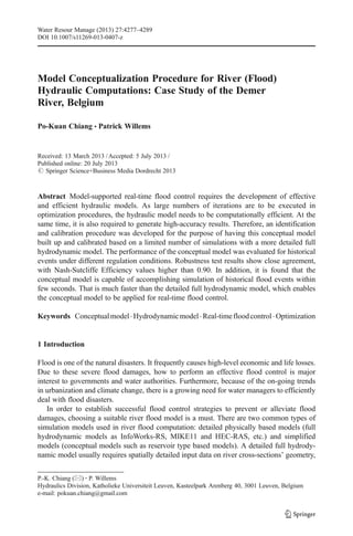
10. 4.1 Calibration and Validation Results
The conceptual model has around 80 variables. For eight selected variables (from up- to
downstream along the river system: vopw1, qA, vs, v2, vzw2, v4, vw2 and vafw), model results are
hereafter evaluated after comparison with the simulation results of the InfoWorks-RS model.
This is done based on the Nash-Sutcliffe efficiency coefficient (EC) (Nash and Sutcliffe 1970).
Figure 3a–h reveal the conceptual model’s calibration and validation results in time series
plots. The variables hopw1, h2, h4 and hafw demonstrate four water levels located at specific
junctions of the river Demer. These four storage nodes receive flows from several branches
and from hydraulic structures. It is seen in the figures and in Table 1 that the water levels of
the two models along the river Demer closely match; the EC values are higher than 0.902 for
all four water levels and four events.
Figure 3b, c and g show the results for gate discharge qA and water levels hs and hw2. It is
important to note that the water level hs interacts with hopw1 (the upstream water level of the
gate) to determine when the reservoir Schulensmeer will be filled. Similar conditions apply
to the water level hw2 that controls the reservoir Webbekom. The water level hs presents
good performance (the four EC values in Table 1 are higher than 0.899). While combining hs
with the above-mentioned good water level hopw1, the gated weir A’s operations and
discharge computations of the conceptual model are close to those of the InfoWorks-RS
model (four EC values for qA=0.976).
Also for the water level hw2, results indicate that the level can be simulated well for all
four events (four EC values for hw2=0.848). The key-point for getting a good result of hw2
was to improve the performance of qK19, based on a careful modelling of the flow-separation
of qvopw in qK19 and qK18 based on the upstream water level hv.
Concerning the computations of the spills (e.g. q_vlo104, qs3, qhs_r and so forth), water
level hzw2 presents the integrated performance of several spills on the right side of the Demer
river. As shown in Fig. 3e and Table 1, the results of hzw2 for the flood event 1998 simulated
by the conceptual model match reasonably well with those run by the InfoWorks-RS model
(EC value equals 0.937). The results for the other three events do not match so well. This
result may be due to the calibrated rating curve of the storage node vzw2, which does not
describe well enough the relation between the very low discharge and the low water level
under the condition of no spill (only inflow qzwopw). Accordingly, the performance is less
good for low water levels in this storage node (three EC values are less than 0.5).
Figure 4a–b provide the evaluations of several peak water levels. As the model results are
aggregated to a 1-h time step, the effect on time delays is not considered here. Hence, the
Table 2 Differences between the two cases of the robustness test and the original case
Original case Case_1 of the
robustness test
Case_2 of the
robustness test
Gated weirs for which operating
rules have been changed in the
robustness test (Case_1
Case_2)
– 10 gated weirs (deducting
gated weirs K18 and K31)
10 gated weirs (deducting
gated weirs K18 and
K31)
Gated weirs with different
operating rules for Case_2
in comparison with Case_1
– Gated weirs K19, K24A
K24B and K30
Particular settings h0 of K18=20.0 h0 of K24A=20.80
h0 of K31=21.5 h0 of K24B=20.13
4286 P.-K. Chiang, P. Willems

11. occurrence of the peak value with respect to the water level or the weir flow is to be fully
decided by its own time series, conceptual or the InfoWorks-RS model.
The comparison of the peak water levels at the selected nodes of the river Demer (hopw1,
h2, h3, h4, h5 and hafw) in the scatter plot of Fig. 4a shows that the six peak water levels are
clustered close to the bisector, thanks to the good accuracy of the v-h relations implemented
in the conceptual model.
For the evaluation of the water levels inside the floodplains, the comparison of the peak
water levels inside the floodplains (hs3, hs4, hs5 and hs_gL) are shown in the scatter plot of
Fig. 4b. As mentioned, except for the 1998 flood event, there were no spill discharges along
the river system. As shown in this figure, except the residual of the peak water levels hs_gL
(−34 cm) in the 1995 flood event and that of the peak water levels hs3 (−44 cm) and hs_gL
(−49 cm) in the 1999 flood event, other residuals of the peak water levels in the four events
are all below ±30 cm.
4.2 Calculation Time Reduction
The CPU time of the conceptual model is between 1.67 and 2.42 s depending on the flood
event, on a PC with Microsoft Windows XP professional, Intel Pentium 4 CPU 2.80 GHz
and 2 GB of RAM. This compares to the much longer CPU time of the full hydrodynamic
model, which ranges between 1 h 56 min and 2 h 31 min. This means that the target of fast-
simulation in this research is achieved. Of course against this strong decrease in CPU time
we have to consider the time it takes for the modeller to develop and calibrate the conceptual
model. The latter effort is, however, a one-time investment, which leads to strong benefits in
all later use of the conceptual model.
4.3 Robustness Test of the Conceptual Model
To evaluate the robustness of the conceptual model, the operating rules were changed for
selected gated weirs. The changes in operating rules were implemented in both the
InfoWorks-RS and the conceptual models and the new model results compared.
The research selected the 1998 flood event for the robustness test because of its severe
inundation conditions. In order to carry out the test, the operating rules of all gated weirs
were reset. For example, the operating rules of the water-level thresholds and the gate
movements were set completely different from those of the original case (but excluding
gated weirs K18 and K31). This was done for 10 gated weirs and two sets of highly different
changes (Case_1 and Case_2) (see Table 2).
Results are evaluated for the same eight variables as in Section 4.1. It is seen in Table 3
that after the large differences in operating rules, the water levels in the conceptual model
match equally well with the InfoWorks-RS results. All EC values for the four water levels
hopw1, h2, h4, hafw and the two cases are equal or higher than 0.923. Table 3 presents good
performances for the Schulensmeer reservoir water level hs (EC=0.983) and the gated weir
discharges qA except for the peak flows (EC=0.917). Moreover, the results for water level
Table 3 EC results for the two robustness test cases
Event hopw1 qA hs h2 hzw2 h4 hw2 hafw
1998 Case_1 0.935 0.917 0.983 0.974 0.886 0.934 0.836 0.970
1998 Case_2 0.956 0.936 0.989 0.970 0.898 0.923 0.914 0.963
Model Conceptualization Procedure for River Hydraulics 4287

12. hw2 indicate that the conceptual model relations controlling hw2, calibrated for the 1998 flood
event, still give good results (EC=0.836) under different flow conditions. Also, the results
of hzw2 simulated by the conceptual model generally match those run by the InfoWorks-RS
model for the two robustness test runs (EC=0.886).
For the peak water levels inside the floodplains (hs3, hs4, hs5 and hs_gL), the residuals of
these levels are for the two cases all below 15 cm.
5 Conclusions and Discussions
This paper demonstrated the designed conceptual river model’s ability to simulate river
hydrodynamic states and flow processes in an accurate and fast way. The EC values for
water levels between the conceptual and full hydrodynamic model results for the four
considered flood events were found to be higher than 0.90 for both calibration and validation
periods, except for the water levels hzw2 and hw2. In order to evaluate the robustness of the
conceptual model, after strong changes were made in these operating rules, EC values higher
than 0.92 were found for the water levels, except for hzw2 and hw2. For these two water
levels, the EC value is a bit lower than 0.90, but still higher than 0.83.
A crucial achievement is that the conceptual model requires only 2.42 s to simulate the
whole 1998 flood event, comparing to 1 h 56 min that the detailed hydrodynamic model
requires to run the same event. As mentioned, the conceptualization procedure is designed to
substantially reduce the calculation time but still maintains high accuracy, while comparing
to the detailed hydrodynamic model. This is to ensure future possible integration in a real-
time flood control operation scheme. This scheme is to optimize the hydraulic-structure
operations with predicted inflows that are calculated by a rainfall-runoff model linked with a
technique to support real time control, such as the Model Predictive Control (MPC)
(Delgoda et al. 2013; Barjas Blanco et al. 2008, 2010).
Further research is, however, required to improve the construction of the conceptual
model. One is to calculate v-h relations with a more efficient (semi-automatic) method, such
as nonlinear/dynamic transfer function identification and calibration procedures (Beven et al.
2009; Villazón Gómez 2011). These procedures may be used to derive the conceptual sub-
model equations by a black-box method, for the purpose of preventing too much time to be
spent in the derivation of these equations. It is also important to note that the conceptual
model developed in this study aims to estimate two 1D variables of the flow only water stage
(or water depth) and flow discharge (or velocity) only. Multi-dimensional hydrodynamic
models can be used for high resolution (spatial and temporal) computation of parameters
such as turbulent kinetic energy and Reynolds stresses that are important, for instance, to
sediment transport, flow-structure interaction, etc. When the latter is needed, the conceptual
model cannot be used.
Acknowledgments The full hydrodynamic InfoWorks-RS model of the Demer basin and the validated
hydrometric data were provided by the Division Operational Water Management of the Flemish Environment
Agency (VMM). We also acknowledge Innovyze for the InfoWorks-RS software and license.
References
Ballesteros-Cánovas JA, Sanchez-Silva M, Bodoque JM, Díez-Herrero A (2013) An integrated approach to flood
risk management: a case study of Navaluenga (Central Spain). Water Resour Manag 27(8):3051–3069
4288 P.-K. Chiang, P. Willems

13. Barjas Blanco T, Willems P, De Moor B, Berlamont J (2008) Flood prevention of the Demer using model
predictive control. Paper presented at the 17th IFAC World Congress, Seoul, South Korea, 6–11 July
Barjas Blanco T, Willems P, Chiang P-K, Cauwenberghs K, Moor B, Berlamont J (2010) Flood regulation by
means of model predictive control. In: Negenborn RR, Lukszo Z, Hellendoorn H (eds) Intelligent
infrastructures. Springer, Dordrecht
Beven K, Young P, Leedal D, Romanowicz R (2009) Computationally efficient flood water level prediction
(with uncertainty). Paper presented at the Flood Risk Management: Research and Practice, London, UK,
30 September–2 October
Chiang P-K, Willems P, Berlamont J (2010) A conceptual river model to support real-time flood control
(Demer River, Belgium). Paper presented at the River Flow 2010 International Conference on Fluvial
Hydraulics, TU Braunschweig, Germany, 8–10 September
Chow V, Maidment D, Mays L (1988) Applied hydrology. Editions McGraw-Hill, New York
Delgoda D, Saleem S, Halgamuge M, Malano H (2013) Multiple model predictive flood control in regulated
river systems with uncertain inflows. Water Resour Manag 27(3):765–790
Fischer A, Rouault P, Kroll S, Van Assel J, Pawlowsky-Reusing E (2009) Possibilities of sewer model
simplifications. Urban Water J 6(6):457–470
Forster S, Chatterjee C, Bronstert A (2008) Hydrodynamic simulation of the operational management of a
proposed flood emergency storage area at the Middle Elbe River. River Res Appl 24(7):900–913
HIC (2003) The Digital Demer: A New and Powerful Instrument for Water Level Management (in Dutch),
Hydrologic Information Service of the Authorities of Flanders, Borgerhout, Belgium
InfoWorks (2006) InfoWorks-RS reference manual, Wallingford Software, MWH Soft. Oxfordshire, UK
Leon A, Kanashiro E, González-Castro J (2013) Fast approach for unsteady flow routing in complex river
networks based on performance graphs. J Hydraul Eng 139(3):284–295
Moore R (2007) The PDM rainfall-runoff model. Hydrol Earth Syst Sci 11(1):483–499
Moore R, Bell V (2002) Incorporation of groundwater losses and well level data in rainfall-runoff models
illustrated using the PDM. Hydrol Earth Syst Sci 6(1):25–38
Nash JE, Sutcliffe JV (1970) River flow forecasting through conceptual models part I—a discussion of
principles. J Hydrol 10(3):282–290
Ngo L, Madsen H, Rosbjerg D, Pedersen C (2008) Implementation and comparison of reservoir operation
strategies for the Hoa Binh Reservoir, Vietnam using the Mike 11 Model. Water Resour Manag
22(4):457–472
Pender G, Neelz S (2007) Use of computer models of flood inundation to facilitate communication in flood
risk management. Environ Hazards 7(2):106–114
Rouault P, Fischer A, Schroeder K, Pawlowsky-Reusing E, Van Assel J (2008) Simplification of dynamic flow
routing models using hybrid modelling approaches—two case studies. Paper presented at the 11th
International Conference on Urban Drainage, Edinburgh, Scotland, UK, 31 August–5 September
Schuurmans J (1997) Control of water levels in open-channels. Ph.D. dissertation, Delft University of
Technology, Delft, The Netherlands
Vaes G (1999) The influence of rainfall and model simplification on combined sewer system design. Ph.D.
dissertation, Katholieke Universiteit Leuven, Leuven, Belgium
Vaes G, Berlamont J (1999) Emission predictions with a multi-linear reservoir model. Water Sci Technol
39:9–16
Villazón Gómez M (2011) Modelling and Conceptualization of Hydrology and River Hydraulics in Flood
Conditions, for Belgian and Bolivian Basins. Ph.D. dissertation, Katholieke Universiteit Leuven, Leuven,
Belgium
Willems P (2010) Parsimonious model for combined sewer overflow pollution. J Environ Eng 136:316
Willems P, Barjas Blanco T, Chiang P-K, Cauwenberghs K, Berlamont J, De Moor B (2008) Evaluation of
river flood regulation by means of model predictive control. Paper presented at the 4th International
Symposium on Flood Defense: Managing Flood Risk, Reliability and Vulnerability, Toronto, Ontario,
Canada, 6–8 May
Yazdi J, Salehi Neyshabouri SAA (2012) A simulation-based optimization model for flood management on a
watershed scale. Water Resour Manag 26(15):4569–4586
Model Conceptualization Procedure for River Hydraulics 4289