
Recommended
Recommended
More Related Content
Similar to WEB APPENDIX 5ACALCULATING BETA COEFFICIENTS5A-1The .docx
Similar to WEB APPENDIX 5ACALCULATING BETA COEFFICIENTS5A-1The .docx (20)
More from melbruce90096
More from melbruce90096 (20)
Recently uploaded
Recently uploaded (20)
WEB APPENDIX 5ACALCULATING BETA COEFFICIENTS5A-1The .docx
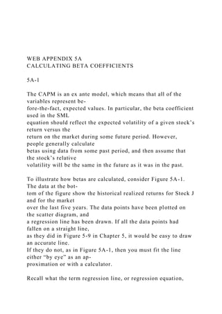
- 1. WEB APPENDIX 5A CALCULATING BETA COEFFICIENTS 5A-1 The CAPM is an ex ante model, which means that all of the variables represent be- fore-the-fact, expected values. In particular, the beta coefficient used in the SML equation should reflect the expected volatility of a given stock’s return versus the return on the market during some future period. However, people generally calculate betas using data from some past period, and then assume that the stock’s relative volatility will be the same in the future as it was in the past. To illustrate how betas are calculated, consider Figure 5A-1. The data at the bot- tom of the figure show the historical realized returns for Stock J and for the market over the last five years. The data points have been plotted on the scatter diagram, and a regression line has been drawn. If all the data points had fallen on a straight line, as they did in Figure 5-9 in Chapter 5, it would be easy to draw an accurate line. If they do not, as in Figure 5A-1, then you must fit the line either “by eye” as an ap- proximation or with a calculator. Recall what the term regression line, or regression equation,
- 2. means: The equation Y � a � bX � e is the standard form of a simple linear regression. It states that the de- pendent variable, Y, is equal to a constant, a, plus b times X, where b is the slope co- efficient and X is the independent variable, plus an error term, e. Thus, the rate of return on the stock during a given time period ( Y ) depends on what happens to the general stock market, which is measured by X � k – M. Once the data have been plotted and the regression line has been drawn on graph paper, we can estimate its intercept and slope, the a and b values in Y � a � bX. The intercept, a, is simply the point where the line cuts the vertical axis. The slope coef- ficient, b, can be estimated by the “rise-over-run” method. This involves calculating the amount by which k – J increases for a given increase in k – M. For example, we ob- serve in Figure 5A-1 that k – J increases from �8.9 to �7.1 percent (the rise) when k –
- 3. M increases from 0 to 10.0 percent (the run). Thus, b, the beta coefficient, can be mea- sured as follows: Note that rise over run is a ratio, and it would be the same if measured using any two arbitrarily selected points on the line. The regression line equation enables us to predict a rate of return for Stock J, given a value of k – M. For example, if k – M � 15%, we would predict k – J � �8.9% � 1.6(15%) � 15.1%. However, the actual return would probably differ from the pre- dicted return. This deviation is the error term, eJ, for the year, and it varies randomly from year to year depending on company-specific factors. Note, though, that the higher the correlation coefficient, the closer the points lie to the regression line, and the smaller the errors. In actual practice, monthly, rather than annual, returns are generally used for k –
- 4. J and k – M, and five years of data are often employed; thus, there would be 5 � 12 � 60 b � Beta � Rise Run � ∆Y ∆X � 7.1 � 1�8.92 10.0 � 0.0 � 16.0 10.0 � 1.6. A P P E N D I X 5 A � C A L C U L AT I N G B E TA C O E F F I C I E N T S 5A App5A_SW_Brigham_778312 1/23/03 5:41 AM Page 5A-1
- 5. 5A-2 data points on the scatter diagram. Also, in practice one would use the least squares method for finding the regression coefficients a and b. This procedure minimizes the squared values of the error terms, and it is discussed in statistics courses. The least squares value of beta can be obtained quite easily with a financial calcu- lator. The procedures that follow explain how to find the values of beta and the slope using either a Texas Instruments, a Hewlett-Packard, or a Sharp financial calculator or a spreadsheet program, such as Microsoft Excel. A P P E N D I X 5 A � C A L C U L AT I N G B E TA C O E F F I C I E N T S F I G U R E 5 A - 1 Calculating Beta Coefficients k _ ∆ Historic Realized Returns on Stock J, kJ(%) Historic Realized Returns on the Market, k (%) 302010
- 6. aJ = Intercept = – 8.9% k = 8.9% + 7.1% = 16% = 10% b = Rise Run = = 16 10 = 1.6J M J J –10 0 –20 –10 10 20 30 40 7.1 Year 3
- 7. Year 4 Year 5Year 1 = aJ + bJkM + eJ = – 8.9 + 1.6k M + eJ k J _ __ Year 2 _ _ M _ M ∆ k _ ∆ k _ ∆ YEAR MARKET (k _ M) STOCK J (k
- 8. _ J) 1 23.8% 38.6% 2 (7.2) (24.7) 3 6.6 12.3 4 20.5 8.2 5 30.6. .. 40.1.... Average k _ 14.9% 14.9% �k _ 15.1% 26.5% App5A_SW_Brigham_778312 1/23/03 5:41 AM Page 5A-2 5A-3 T E X A S I N S T R U M E N T S BA- I I P L U S 1. Press until “STAT” shows in the display. 2. Enter the first X value ( k – M � 23.8 in our example), press , and then enter the first Y value ( k – J � 38.6) and press .
- 9. 3. Repeat Step 2 until all values have been entered. 4. Press to find the value of Y at X � 0, which is the value of the Y inter- cept (a), �8.9219, and then press to display the value of the slope (beta), 1.6031. 5. You could also press to obtain the correlation coefficient, r, which is 0.9134. Putting it all together, you should have this regression line: k – J � �8.92 � 1.60k – M. r � 0.9134. H E W L E T T - PA C K A R D 1 0 B I I 1 1. Press to clear your memory registers. 2. Enter the first X value ( k – M � 23.8 in our example), press , and then enter the first Y value ( k – J � 38.6) and press . Be sure to enter the X variable
- 10. first. 3. Repeat Step 2 until all values have been entered. 4. To display the vertical axis intercept, press 0 . Then �8.9219 should appear. 5. To display the beta coefficient, b, press . Then 1.6031 should appear. 6. To obtain the correlation coefficient, press and then to get r � 0.9134. Putting it all together, you should have this regression line: k – J � �8.92 � 1.60k – M. r � 0.9134. S H A R P E L - 7 3 3 1. Press until “STAT” shows in the lower right corner of the display. 2. Press to clear all memory registers. 3. Enter the first X value (k – M � 23.8 in our example) and press . (This is the RM key; do not press the second F key at all.) Then enter the
- 11. first Y value (k – J � 38.6), and press . (This is the M� key; again, do not press the second F key). 4. Repeat Step 3 until all values have been entered. DATA (x,y) CA2nd F Mode2nd F SWAPx̂ ,r SWAP ŷ,m ∑� INPUT Clear all Corr2nd x � y b/a2nd ∑� x � y
- 12. Mode2nd A P P E N D I X 5 A � C A L C U L AT I N G B E TA C O E F F I C I E N T S 1 The Hewlett-Packard 17B calculator is even easier to use. If you have one, see Chapter 9 of the Owner’s Manual. App5A_SW_Brigham_778312 1/23/03 5:41 AM Page 5A-3 5A-4 5. Press a to find the value of Y at X � 0, which is the value of the Y intercept (a), �8.9219, and then press to display the value of the slope (beta), 1.6031. 6. You can also press to obtain the correlation coefficient, r, which is 0.9134. Putting it all together, you should have this regression line: k – J � �8.92 � 1.60k – M.
- 13. r � 0.9134. M I C R O S O F T E X C E L 1. Manually enter the data for the market and Stock J into the spreadsheet as shown below. 2. Access Microsoft Excel’s Regression tool from the Data Analysis package in the Tools menu (Tools � Data Analysis � Regression). If you do not have the Data Analysis package, you will have to add the Analysis ToolPak, by accessing Tools � Add-Ins. The regression dialog box that appears requires you to input the Y and X variable ranges, and it has additional options pertaining to the output that is to be produced and where it shall be displayed. In this example regarding Stock J, the “Input Y Range:” prompt requires cells C2:C6 be entered as the dependent variable of the regression. Similarly, the “Input X Range:” prompt requires cells B2:B6 be entered as the independent variable. r2nd F b2nd F a2nd F A P P E N D I X 5 A � C A L C U L AT I N G B E TA C O E F F I C I E N T S
- 14. App5A_SW_Brigham_778312 1/23/03 5:41 AM Page 5A-4 5A-5 For the purposes of this example, none of the additional options are chosen, and the regression output relies upon the default selection, which is to be dis- played on an additional worksheet. 3. Select “OK” to perform the indicated regression. 4. A section of the output generated from the regression of Stock J’s return on the market return is shown below: In this simple regression, the multiple R statistic is equivalent to the correla- tion coefficient obtained in the other regression procedures described. Hence, the correlation coefficient, r, is 0.91339175. 5. In the last section of the output, it is found that the intercept of the regression line is �0.0892194, and the beta coefficient is 1.60309159. These results agree with those obtained previously with financial calculators, except that the inter- cept is �0.089219 instead of �8.9219. The reason for this difference is that the returns were entered as whole numbers in the calculator, but were expressed as percentages in the spreadsheet. It is simply a matter of scale and does not have
- 15. a real effect on results. 6. The remainder of the regression output concerns the reliability of the estimates made and these additional data are more fully explained in statistics courses. Putting it all together, you should have this regression line: k – J � �8.92 � 1.60k – M. r � 0.9134. As illustrated, spreadsheet programs yield the same results as a calculator, however the spreadsheet is more flexible and allows for a more thorough analysis. First, the file can be retained, and when new data become available, they can be added and a new beta can be calculated quite rapidly. Second, the regression output can include graphs and statistical information designed to give us an idea of how stable the beta coefficient is. In other words, while our beta was calculated to be 1.60, the “true beta” might actually be higher or lower, and the regression output can give us an idea of how large the error might be. Third, the spreadsheet can be used to calculate
- 16. A P P E N D I X 5 A � C A L C U L AT I N G B E TA C O E F F I C I E N T S App5A_SW_Brigham_778312 1/23/03 5:41 AM Page 5A-5 5A-6 returns data from historical stock price and dividend information, and then the re- turns can be fed into the regression routine to calculate the beta coefficient. This is important, because stock market data are generally provided in the form of stock prices and dividends, making it necessary to calculate returns. This can be a big job if a number of different companies and a number of time periods are involved. P R O B L E M S You are given the following set of data: H I S T O R I C A L R A T E S O F R E T U R N ( k _ ) YEAR STOCK Y (k _ Y) NYSE (k _ M)
- 17. 1 3.0% 4.0% 2 18.2 14.3 3 9.1 19.0 4 (6.0) (14.7) 5 (15.3) (26.5) 6 33.1 37.2 7 6.1 23.8 8 3.2 (7.2) 9 14.8 6.6 10 24.1 20.5 11 18.0... 30.6 Mean 9.8% 9.8% �k _ 13.8 19.6 a. Construct a scatter diagram graph (on graph paper) showing the relationship between re- turns on Stock Y and the market as in Figure 5A-1; then draw a freehand approximation of the regression line. What is the approximate value of the beta coefficient? (If you have a calculator with statistical functions or a computer, use it to calculate beta.) b. Give a verbal interpretation of what the regression line and the beta coefficient show about Stock Y’s volatility and relative riskiness as compared with other stocks. c. Suppose the scatter of points had been more spread out but the regression line was exactly where your present graph shows it. How would this affect (1)
- 18. the firm’s risk if the stock were held in a 1-asset portfolio and (2) the actual risk premium on the stock if the CAPM held exactly? How would the degree of scatter (or the correlation coefficient) affect your confidence that the calculated beta will hold true in the years ahead? d. Suppose the regression line had been downward sloping and the beta coefficient had been negative. What would this imply about (1) Stock Y’s relative riskiness and (2) its probable risk premium? e. Construct an illustrative probability distribution graph of returns (see Figure 5-7) for port- folios consisting of (1) only Stock Y, (2) 1 percent each of 100 stocks with beta coefficients similar to that of Stock Y, and (3) all stocks (that is, the distribution of returns on the mar- ket). Use as the expected rate of return the arithmetic mean as given previously for both Stock Y and the market, and assume that the distributions are normal. Are the expected re- turns “reasonable”— that is, is it reasonable that k̂ Y � k̂ M � 9.8%? f. Now, suppose that in the next year, Year 12, the market return was 27 percent, but Firm Y increased its use of debt, which raised its perceived risk to investors. Do you think that the return on Stock Y in Year 12 could be approximated by this historical characteristic line? k̂ Y � 3.8% � 0.62(k̂ M) � 3.8% � 0.62(27%) � 20.5%.
- 19. A P P E N D I X 5 A � C A L C U L AT I N G B E TA C O E F F I C I E N T S 5A-1 Beta coefficients and rates of return App5A_SW_Brigham_778312 1/23/03 5:41 AM Page 5A-6 5A-7 g. Now, suppose k _ Y in Year 12, after the debt ratio was increased, had actually been 0 per- cent. What would the new beta be, based on the most recent 11 years of data (that is, Years 2 through 12)? Does this beta seem reasonable— that is, is the change in beta consistent with the other facts given in the problem? You are given the following historical data on market returns, k _ M, and the returns on Stocks A and B, k _ A and k _ B:
- 20. YEAR k _ M k _ A k _ B 1 29.00% 29.00% 20.00% 2 15.20 15.20 13.10 3 (10.00) (10.00) 0.50 4 3.30 3.30 7.15 5 23.00 23.00 17.00 6 31.70 31.70 21.35 kRF, the risk-free rate, is 9 percent. Your probability distribution for kM for next year is as follows: PROBABILITY kM 0.1 (14%) 0.2 0 0.4 15 0.2 25 0.1 44 a. Determine graphically the beta coefficients for Stocks A and B. b. Graph the Security Market Line, and give its equation. c. Calculate the required rates of return on Stocks A and B. d. Suppose a new stock, C, with k̂ C � 18 percent and bC � 2.0,
- 21. becomes available. Is this stock in equilibrium; that is, does the required rate of return on Stock C equal its ex- pected return? Explain. If the stock is not in equilibrium, explain how equilibrium will be restored. A P P E N D I X 5 A � C A L C U L AT I N G B E TA C O E F F I C I E N T S 5A-2 Security Market Line App5A_SW_Brigham_778312 1/23/03 5:41 AM Page 5A-71