This document presents a decision problem faced by a manufacturer. The manufacturer produces items that have a probability of being defective. These items are formed into batches of 150. The manufacturer can either screen each item in a batch to check for defects at a cost of $10 per item screened, or use the items directly without screening and incur a cost of $100 per defective item that makes it through. Based on the given probabilities of good vs. bad quality batches, the expected costs per batch are calculated for each option. A decision tree is constructed to model the problem, taking into account the option to first test a single randomly selected item from the batch before deciding whether to screen the entire batch or not. The optimal strategy is determined to be

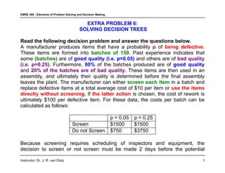
1. EMSE 269 - Elements of Problem Solving and Decision Making
Instructor: Dr. J. R. van Dorp 1
EXTRA PROBLEM 6:
SOLVING DECISION TREES
Read the following decision problem and answer the questions below.
A manufacturer produces items that have a probability of .
p being defective
These items are formed into . Past experience indicates that
batches of 150
some are of and others are of
(batches) good quality (i.e. p=0.05) bad quality
(i.e. p=0.25). Furthermore, of the batches produced are of
80% good quality
and These items are then used in an
20% of the batches are of bad quality.
assembly, and ultimately their quality is determined before the final assembly
leaves the plant. The manufacturer can either in a batch and
screen each item
replace defective items at a total average cost of $10 per item or use the items
directly without screening. the latter action
If is chosen, the cost of rework is
ultimately $100 per defective item. For these data, the costs per batch can be
calculated as follows:
p = 0.05 p = 0.25
Screen $1500 $1500
Do not Screen $750 $3750
Because screening requires scheduling of inspectors and equipment, the
decision to screen or not screen must be made 2 days before the potential

2. EMSE 269 - Elements of Problem Solving and Decision Making
Instructor: Dr. J. R. van Dorp 2
screening takes place. However, the manufactures may take one item taken
from a batch and sent it to a laboratory, and the test results (defective or non-
defective) can be reported must be
before the screen/no-screen decision
made. After the laboratory test, The
the tested item is returned to its batch.
cost of this initial inspection is $125. Also note that the probability that a random
sample item is defective is
0.8 * 0.05 + 0.2 * 0.25 = 0.09,
and the probability that an item in a lot is of good quality given a randomly
sampled item is defective is 0.444 and the probability that an item in a lot is
of good quality given a randomly sampled item is not defective is 0.835.
The manufactur wants to minimize his or her cost.
A. Derive the cost figures in the table above. Clearly show your calculations.
p = 0.05 p = 0.25
Screen 150*$10 = $1500 150*$10 = $1500
Do not Screen 150*0.05*$100 = $750 150*0.25*$100 = $3750
B. What Law of Probability was used in deriving:

3. EMSE 269 - Elements of Problem Solving and Decision Making
Instructor: Dr. J. R. van Dorp 3
Pr(Randomly Sampled Item is Defective)
Pr(Sample Item is Defective|Batch of Good Quality) =0.05
Pr(Sample Item is Defective|Batch of Bad Quality) =0.25
Pr(Batch of Good Quality)=0.80 Pr(Batch of Bad Quality)=0.20
Pr(Randomly Sampled Item is Defective) =
Pr(Sample Item is Defective|Batch of Good Quality)Pr(Batch of Good Quality)+
Pr(Sample Item is Defective|Batch of Bad Quality)Pr(Batch of Bad Quality)=
0.05*0.8 + 0.25*0.2=0.09
Hence, THE LAW OF TOTAL PROBABILITY was used.

4. EMSE 269 - Elements of Problem Solving and Decision Making
Instructor: Dr. J. R. van Dorp 4
C. Show that:
Pr(Batch of Good Quality|Sampled Item is Defective) = 0.444
Pr(Batch of Good Quality|Sampled Item is Not Defective) = 0.835
FKU œ à WMH œ
"Batch of Good Quality" "Sampled Item is Defective";
= "Sampled Item is Not Defective"
WMH
T <ÐFKU WMHÑ œ œ
| T <ÐWMHlFKUÑT <ÐFKUÑ
T <ÐWMHÑ
!Þ!&†!Þ)!
!Þ!* œ !Þ%%%
T <ÐFKU WMHÑ œ
| T <ÐWMHlFKU ÑT <ÐFKUÑ
T <ÐWMHÑ
œ œ !Þ)$&
Ð"!Þ!&ц!Þ)!
Ð"!Þ!*Ñ

5. EMSE 269 - Elements of Problem Solving and Decision Making
Instructor: Dr. J. R. van Dorp 5
D. Calculate and show your calculations:
FKU œ à WMH œ
"Batch of Bad Quality" "Sampled Item is Not Defective"
Pr(Bad Quality|Sampled Item is Defective) = ?
Pr(Bad Quality|Sampled Item is Not Defective) = ?
T <ÐFKU WMHÑ œ "  T <ÐFKU WMHÑ œ
| |
"  !Þ%%% œ !Þ&&'
T <ÐFKU WMHÑ œ "  T <ÐFKU WMHÑ œ
| |
"  !Þ)$& œ !Þ"'&

6. EMSE 269 - Elements of Problem Solving and Decision Making
Instructor: Dr. J. R. van Dorp 6
E. Model the decision problem in a decision tree and fill in ALL the details
Test Item?
Screen?
Passed Test
Failed Test
Screen?
Screen?
No Test
Test
No Screen
Batch of Good Quality
Batch of Bad Quality
Batch of Good Quality
Batch of Bad Quality
Batch of Good Quality
Batch of Bad Quality
No Screen
No Screen
Screen
Screen
Screen
(0.80)
(0.20)
(0.835)
(0.165)
(0.444)
(0.566)
(0.91)
(0.09)
$125
$1500
$1500
$1500
$750
$750
$750
$3750
$3750
$3750
$875
$875
$750
$3750
$1500
$1625
$1625
$3875
$3875
COST

7. EMSE 269 - Elements of Problem Solving and Decision Making
Instructor: Dr. J. R. van Dorp 7
F. How many cumulative risk profiles can be drawn for the decision tree under
E? Provide an Explanation.
Test Item?
Screen?
Passed Test
Failed Test
Screen?
Screen?
No Test
Test
No Screen
Batch of Good Quality
Batch of Bad Quality
Batch of Good Quality
Batch of Bad Quality
Batch of Good Quality
Batch of Bad Quality
No Screen
No Screen
Screen
Screen
Screen
(0.80)
(0.20)
(0.835)
(0.165)
(0.444)
(0.566)
(0.91)
(0.09)
$125
$1500
$1500
$1500
$750
$750
$750
$3750
$3750
$3750
$875
$875
$750
$3750
$1500
$1625
$1625
$3875
$3875
COST
Upper Part: 4 , , ,
(T,{NS,NS}) (T,{S,S}) (T,{NS,S}) (T,{S,NS})
Lower Part: 2 , Total: 6 Strategies
(NT,NS) (NT, S)

8. EMSE 269 - Elements of Problem Solving and Decision Making
Instructor: Dr. J. R. van Dorp 8
G. Solve the tree under E using EMV and clearly show your calculations in the
tree under E
Test Item?
Screen?
Passed Test
Failed Test
Screen?
Screen?
No Test
Test
No Screen
Batch of Good Quality
Batch of Bad Quality
Batch of Good Quality
Batch of Bad Quality
Batch of Good Quality
Batch of Bad Quality
No Screen
No Screen
Screen
Screen
Screen
(0.80)
(0.20)
(0.835)
(0.165)
(0.444)
(0.566)
(0.91)
(0.09)
$125
$1500
$1500
$1500
$750
$750
$750
$3750
$3750
$3750
$875
$875
$750
$3750
$1500
$1625
$1625
$3875
$3875
COST
$1369.51
$1625
$1392.50
$1369.51
$2541.67
$1350
$1350
$1350

9. EMSE 269 - Elements of Problem Solving and Decision Making
Instructor: Dr. J. R. van Dorp 9
H. Describe in words the optimal decision strategy.
Do not Sample an Item Randomly from a Batch for Testing,
and Do Not Screen the entire Batch
(No Test, No Screen in the Decision Tree)

10. EMSE 269 - Elements of Problem Solving and Decision Making
Instructor: Dr. J. R. van Dorp 10
I. Draw the Cumulative Risk Profile for each alternative of the immediate
decision, taking optimal decisions from thereon. What can you conclude with
respect to dominance considerations? (Hint: You should be drawing 2
Cumulative Risk Profiles).
Test Item?
Screen?
Passed Test
Failed Test
Screen?
Screen?
No Test
Test
No Screen
Batch of Good Quality
Batch of Bad Quality
Batch of Good Quality
Batch of Bad Quality
No Screen
Screen
(0.80)
(0.20)
(0.835)
(0.165)
(0.91)
(0.09)
$125
$1500
$750
$750
$3750
$3750
$875
$750
$3750
$1625
$3875
COST
$1392.50

11. EMSE 269 - Elements of Problem Solving and Decision Making
Instructor: Dr. J. R. van Dorp 11
Strategy: Test Random Item and If Item Passed Test then do not Screen the
entire Batch and if Item Failed Test then Screen the entire Batch
T < G9=> œ )(& œ !Þ*"‡!Þ)$& œ !Þ('!
( )
T < G9=> œ "'#& œ !Þ!*
( )
T < G9=> œ $)(& œ !Þ*"‡!Þ"'& œ !Þ"&!
( )
T <ÐG9=> Ÿ )(&Ñ œ !Þ('!
T <ÐG9=> Ÿ "'#&Ñ œ !Þ('!  !Þ!* œ !Þ)&
T <ÐG9=> Ÿ $)(&Ñ œ !Þ)&  !Þ"& œ "Þ!!!
Strategy: Do not Test Random Item and Do not Screen the Entire Batch
T < G9=> œ (&! œ !Þ)!
( )
T < G9=> œ $(&! œ !Þ#!
( )
T <ÐG9=> Ÿ (&!Ñ œ !Þ)!
T <ÐG9=> Ÿ $(&!Ñ œ !Þ)!  !Þ#! œ "Þ!!

12. EMSE 269 - Elements of Problem Solving and Decision Making
Instructor: Dr. J. R. van Dorp 12
0.0
0.1
0.2
0.3
0.4
0.5
0.6
0.7
0.8
0.9
1.0
0.0 $1000 $2000 $3000 $4000
$750
$750 $825
$825 $1625
$1625 $3750
$3750 $3875
$3875
0.76
0.76
0.80
0.80
0.85
0.85
CUMULATIVE RISK PROFILES CROSS. HENCE, NO DETERMINISTIC
DOMINANCE AND NO STOCHASTIC DOMINANCE