Download as PDF, PPTX


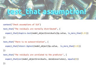
![Tests pass!
> test_file("./tests/test_slr.R")
Check assumptions of SLR : [1] "units_sold ~ price"
...
!](https://image.slidesharecdn.com/craftsmanship-140915105019-phpapp01/85/Assumptions-Check-yo-self-before-you-wreck-yourself-22-320.jpg)
![Psych.
> test_file("./tests/test_slr.R")
Check assumptions of SLR : [1] "units_sold ~ price"
1..
!!
1. Failure(@test_slr.R#12): The residuals are normally distributed
------------------------
shapiro.test(model_object$residuals)$p.value not more than 0.05. Difference: 0.05
!](https://image.slidesharecdn.com/craftsmanship-140915105019-phpapp01/85/Assumptions-Check-yo-self-before-you-wreck-yourself-23-320.jpg)


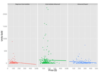
![# Automagically explore SLR with common functional forms
candidate_models = list(linear = 'units_sold ~ price',
loglog = 'log(units_sold + 1) ~ log(price + 1)',
linearlog = 'units_sold ~ log(price + 1)',
loglinear = 'log(units_sold + 1) ~ price')
!
run = function(candidate_models, input_data) {
forecasts = list()
test_input = data.frame(price = 0:1000)
!
# Forecast
for (model in candidate_models) {
test_environment = new.env()
!
# Generate the forecast
forecasts[[model]] = generate_forecast(model, input_data)
!
# Save off current value of things for testing
assign("model", forecasts[[model]], envir = test_environment)
assign("errors", forecasts[[model]]$residuals, envir = test_environment)
assign("covariate", input_data$price, envir = test_environment)
assign("label", model, envir = test_environment)
!
save(test_environment, file = 'env_to_test.Rda')
!
# Run assumption tests
test_file("./tests/test_slr.R")
!
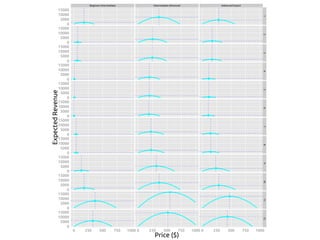
#### OPTIMIZE PRICE!!! ####
opt_results = optimizer(forecasts[[model]], test_input)
!
# Multiply the predicted demand by the price for expected revenue
opt_results$expected_revenue = test_data$price * opt_results$predicted_units_sold
!
pdf(paste(model, “.pdf”, sep = ‘’))
plot_price(opt_results)
!
}
!
return(forecasts)
!
}](https://image.slidesharecdn.com/craftsmanship-140915105019-phpapp01/85/Assumptions-Check-yo-self-before-you-wreck-yourself-30-320.jpg)
![rut roh…
> run(candidate_models, slr_data)
Check assumptions of SLR : [1] "units_sold ~ price"
1..
!!
1. Failure(@test_slr.R#12): The residuals are normally distributed ---------------------------------
shapiro.test(linear$residuals)$p.value not more than 0.05. Difference: 0.05
!
Check assumptions of SLR : [1] "log(units_sold + 1) ~ log(price + 1)"
1.2
!!
1. Failure(@test_slr.R#12): The residuals are normally distributed ---------------------------------
shapiro.test(linear$residuals)$p.value not more than 0.05. Difference: 0.05
!
2. Failure(@test_slr.R#24): The residuals are unrelated to the predictor ---------------------------
cor(test_environment$errors, test_environment$covariate) not equal to 0
Mean absolute difference: 0.05545615
!
Check assumptions of SLR : [1] "units_sold ~ log(price + 1)"
1.2
!!
1. Failure(@test_slr.R#12): The residuals are normally distributed ---------------------------------
shapiro.test(linear$residuals)$p.value not more than 0.05. Difference: 0.05
!
2. Failure(@test_slr.R#24): The residuals are unrelated to the predictor ---------------------------
cor(test_environment$errors, test_environment$covariate) not equal to 0
Mean absolute difference: 0.04201906
!
Check assumptions of SLR : [1] "log(units_sold + 1) ~ price"
1..
!!
1. Failure(@test_slr.R#12): The residuals are normally distributed ---------------------------------
shapiro.test(linear$residuals)$p.value not more than 0.05. Difference: 0.05](https://image.slidesharecdn.com/craftsmanship-140915105019-phpapp01/85/Assumptions-Check-yo-self-before-you-wreck-yourself-31-320.jpg)


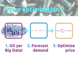
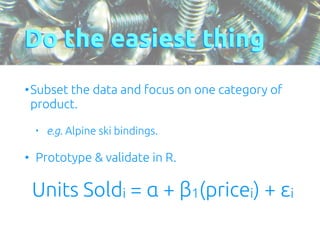
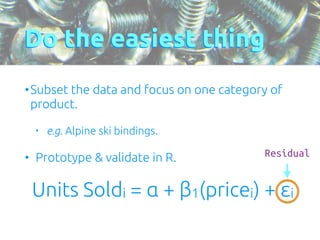
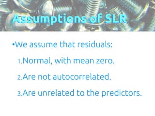
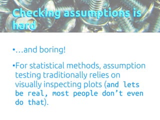
The document discusses the process of price optimization using data science techniques, emphasizing the importance of making sound assumptions and validating them through statistical testing. It outlines steps for harvesting big data, forecasting demand, and optimizing pricing while identifying potential issues with statistical assumptions related to linear regression models. The presentation concludes with a reminder to start with simple approaches and gradually build up complexity, reinforcing the necessity of testing assumptions in data analysis.